Article

Evaluating the Spectral Indices Efficiency to Quantify Daytime Surface Anthropogenic Heat Island Intensity: An Intercontinental Methodology

1
Department of Remote Sensing and GIS, Faculty of Geography, University of Tehran, Tehran 14178-53933, Iran
2
Faculty of Agriculture and Natural Resources, University of Mohaghegh Ardabili, Ardabil 56199-13131, Iran
3
Institute of Geography (Landscape Ecology), Humboldt University of Berlin, Rudower Chaussee 16, 12489 Berlin, Germany
4
Department of Irrigation and Drainage, Tarbiat Modares University, Tehran 14115-336, Iran
*
Author to whom correspondence should be addressed.
Remote Sens. 2020, 12(17), 2854; https://doi.org/10.3390/rs12172854
Submission received: 11 August 2020 / Revised: 30 August 2020 / Accepted: 31 August 2020 / Published: 2 September 2020

Abstract

:
The surface anthropogenic heat island (SAHI) phenomenon is one of the most important environmental concerns in urban areas. SAHIs play a significant role in quality of urban life. Hence, the quantification of SAHI intensity (SAHII) is of great importance. The impervious surface cover (ISC) can well reflect the degree and extent of anthropogenic activities in an area. Various actual ISC (AISC) datasets are available for different regions of the world. However, the temporal and spatial coverage of available and accessible AISC datasets is limited. This study was aimed to evaluate the spectral indices efficiency to daytime SAHII (DSAHII) quantification. Consequently, 14 cities including Budapest, Bucharest, Ciechanow, Hamburg, Lyon, Madrid, Porto, and Rome in Europe and Dallas, Seattle, Minneapolis, Los Angeles, Chicago, and Phoenix in the USA, were selected. A set of 91 Landsat 8 images, the Landsat provisional surface temperature product, the High Resolution Imperviousness Layer (HRIL), and the National Land Cover Database (NLCD) imperviousness data were used as the AISC datasets for the selected cities. The spectral index-based ISC (SIISC) and land surface temperature (LST) were modelled from the Landsat 8 images. Then, a linear least square model (LLSM) obtained from the LST-AISC feature space was applied to quantify the actual SAHII of the selected cities. Finally, the SAHII of the selected cities was modelled based on the LST-SIISC feature space-derived LLSM. Finally, the values of the coefficient of determination (R2) and the root mean square error (RMSE) between the actual and modelled SAHII were calculated to evaluate and compare the performance of different spectral indices in SAHII quantification. The performance of the spectral indices used in the built LST-SIISC feature space for SAHII quantification differed. The index-based built-up index (IBI) (R2 = 0.98, RMSE = 0.34 °C) and albedo (0.76, 1.39 °C) performed the best and worst performance in SAHII quantification, respectively. Our results indicate that the LST-SIISC feature space is very useful and effective for SAHII quantification. The advantages of the spectral indices used in SAHII quantification include (1) synchronization with the recording of thermal data, (2) simplicity, (3) low cost, (4) accessibility under different spatial and temporal conditions, and (5) scalability.

Graphical Abstract

1. Introduction

The rapid and often uncontrolled growth of urbanization and built-up development over the past years has caused a large number of environmental, climatic, and socio-economic problems at local, regional, and global scales [1,2,3,4]. One of the most important environmental challenges in urban areas is the increase in air and land surface temperature (LST) as a result of a lack of vegetation, the widespread use of impervious surfaces, the increased thermal diffusivity of urban materials, the low solar reflectance of urban materials, urban geometries that trap heat and slow wind speeds, increased levels of air pollution, and increased energy use; these factors create surface urban heat islands (SUHIs) [5,6,7,8].
SUHIs are one of the most common urban phenomena; in a SUHI the temperature of urban areas, and city centers in particular, is higher than the temperature of the surrounding rural areas [9,10]. Several studies have investigated the impact of SUHIs on urban flora [11], climate [12], pollutant concentrations [13], air quality [14,15], human health and heat-related deaths [16], global warming [17], thermal comfort [18,19], energy consumption [20], and socioeconomic and environmental impacts [21]; thus, SUHIs play a large role in the quality of urban life [22,23]. Due to these negative effects and considering that rapid population growth is expected in the near future, it will become increasingly important to monitor, predict, and recognize SUHI patterns to improve the quality of urban life [24,25,26,27].
Many factors contribute to SUHI morphology and intensity in a city. These factors can be divided into two main types of factors: (a) uncontrollable factors, such as wind speed, cloudiness, humidity, season, and anti-cyclonic conditions and (b) controllable factors, such as geometry, structural and biophysical characteristics of urban/non-urban areas, and anthropogenic activities and their subsequent impacts, e.g., air pollution [28,29,30,31,32,33]. Based on the effect on the surface energy balance, the factors contributing to SUHI formation in the city can be grouped into five main sets of factors: (a) anthropogenic heat enhancers, (b) evaporation reducers, (c) heat storage enhancers, (d) net radiation enhancers, and (e) convection reducers [31,34].
According to the above perspectives, the anthropogenic heat flux (AHF) in a city majorly contributes to the increase in SUHI intensity (SUHII) [6,35,36]. AHF is released to human activity and comes from many sources, including appliances, buildings, transportation, lighting, industrial and manufacturing processes, and even people themselves, which convert energy into AHF [36,37,38,39,40].
Analyzing the contribution of AHF to urban temperature can help to reduce the uncertainties in our quantitative and qualitative knowledge of the SUHII [35]. Additionally, due to excessive population growth, urban area expansion, increased energy consumption, increasing human activities, and increasing anthropogenic heat in major global cities, monitoring and recognizing surface anthropogenic heat islands (SAHIs) are very important [6,37,38,41]. The effects of human activity on air temperature, LST, and energy balance equilibrium and their spatial distribution in the urban environment have been studied and modelled in various studies.
Hu, et al. [42] found that no AHF was generated by nonartificial surfaces; only some impervious surface layers were involved in AHF, such as roads, residential structures (low-rise and high-rise dwellings), industrial structures (factories), airports, commercial areas, and so on. Zhang, Balzter and Wu [35] analyzed the spatial distribution of AHF across land cover types, impervious surface areas, and vegetation coverages. It is apparent that the contribution of AHF is lower in suburban areas and higher in high-density urban areas. The variation in AHF is influenced by urban expansion, land-cover change, and increasing energy consumption. Chen and Hu [41] showed that the spatial distribution of AHF results is generally centered on urban areas and gradually decreases towards suburbs. The spatial pattern of the AHF results within urban areas corresponds well to the distribution of population density, building density, and industrial districts. Wang, Hu, Chen and Yu [38] showed that high-value AHF areas are mainly distributed at airports, railway stations, industrial areas, and commercial centers. Previous studies have shown that AHF differs across different land covers and is highly correlated with impervious surface cover (ISC) [38,41,42,43,44,45,46,47].
Firozjaei, et al. [48] developed a physical approach based on a triple-source surface energy balance (triple-SEB) to model LST due to AHF and SAHI intensity (SAHII). They showed that LST due to AHF in Beijing, Tehran, Istanbul, Athens, Atlanta, and Los Angeles over the past three decades ranged from 0.72, 0.58, 0.64, 0.61, 0.55, and 2.02 to 2.76, 2.32, 1.19, 1.66, 1.73, and 2.99 °C, respectively. Additionally, the SAHII value for these cities increased by 1.32, 0.95, 0.98, 0.95, 0.92, and 0.73 °C, respectively. They showed a high spatial correlation between ISC and LST due to AHF. Single date Landsat 8 images in each year were used to model LST due to AHF and SAHII variations over the past three decades.
Various studies have shown that the ISC can well reflect the degree and extent of human activity in an area. However, the accurate extraction of ISC from satellite imagery is a major challenge. Different actual ISC (AISC) datasets are available for different parts of the world. For example, the National Land Cover Database (NLCD) dataset represents surface imperviousness information for the United States of America (USA) for 1992, 2001, 2006, 2011, and 2016. The High Resolution Imperviousness Layer (HRIL) database also contains information on European impervious surfaces for 2006, 2009, 2012, and 2015. However, the temporal and spatial coverage of available and accessible AISC datasets are limited. Therefore, it is necessary to use remote sensing (RS)-based indices and methods to extract ISC information for different environmental applications.
In previous studies, various spectral indices and methods, such as the urban index (UI) [49,50], the normalized difference bareness index (NDBaI) [50], the normalized difference built-up index (NDBI) [51], the index-based built-up index (IBI) [52], the modified NDBI [53], the band ratio for built-up area (BRBA) and the normalized built-up area index (NBAI) [54], the built-up index (BUI) [55], the new built-up index (NBI) [56], the bare soil index (BI) [57], soil index (SI), normalized built-up and bare soil index (NBBSI) [58], the built-up area extraction method (BAEM) [59], the enhanced built-up and bareness index (EBBI) [60], and the automated built-up extraction index (ABEI) [61], have been proposed for the extraction of built-up and impervious lands. The advantages of these indices include (1) synchronization with the recording of thermal data, (2) simplicity, (3) low cost, (4) accessibility under different spatial and temporal conditions, and (5) scalability [61]. Therefore, using these indices can be useful for SAHI quantification.
The objective of this study was to evaluate the spectral indices efficiency to daytime SAHII (DSAHII) quantification. The innovations and distinguishing features of the present study are (1) SAHII modelling based on spectral indices and (2) evaluation of the DSAHII of some European and American cities.

2. Study Area

To evaluate and compare the performance of different spectral indices through SAHI modelling, 14 test sites with different conditions were selected. The test sites were Budapest, Bucharest, Ciechanow, Hamburg, Lyon, Madrid, Porto, and Rome in Europe and Minneapolis, Dallas, Phoenix, Los Angeles, Chicago, and Seattle in the USA. The geographical locations of these cities are shown in Figure 1.
To select these cities, various criteria including (1) geographical conditions, (2) surface characteristics, (3) climatic conditions, (4) varied physical size, and (5) population density were considered [61,62]. The characteristics of selected cities are summarized in Table 1.

3. Data and Methods

3.1. Data

A set of Landsat 8 satellite image data, MODIS products, and AISC datasets were used. Details on the data used are shown in Table 2.
Landsat 8 images were used to model surface properties such as LST and various built-up indices. According to previous studies, Landsat images are suitable data for modelling and monitoring environmental conditions due to their spatial, temporal, and radiometric resolution [24,31]. The characteristics of the Landsat 8 bands are given in Table 3.
The Landsat Provisional Surface Temperature product with 30 m spatial resolution was used for USA cities. This product is generated from the Landsat Collection 1 Level-1 thermal infrared bands, Top of Atmosphere (TOA) Reflectance, Advanced Spaceborne Thermal Emission and Reflection Radiometer (ASTER) Global Emissivity Database (GED) data, ASTER Normalized Difference Vegetation Index (NDVI) data, and atmospheric profiles of geopotential height, specific humidity, and air temperature were extracted from reanalysis data (https://www.usgs.gov/land-resources/nli/landsat/landsat-surface-temperature).
MOD11A1 and MOD07 products were also used to calculate and evaluate LST based on Landsat 8 images for European cities. The HRLI and NCLD datasets were used as the AISC for European and American cities, respectively.

3.2. Methods

In this study, a conceptual model with four main sections was designed (Figure 2). First, the Landsat 8 images were preprocessed. Second, the spectral index-based ISC (SIISC) and LST were modelled based on different built-up indices (as described in Section 3.2.2), tasseled cap transformation (TCT), the biophysical composition index (BCI), and a Single-channel algorithm, from the Landsat 8 images. Additionally, a linear least squares model (LLSM) was obtained from the LST-AISC feature space was applied to quantify the actual DSAHII of the selected cities. In the third step, the DSAHII of selected cities was modelled based on the LST-SIISC feature space-derived LLSM. Finally, the value of the coefficient of determination (R2) and the root mean square error (RMSE) between the actual and modelled DSAHII were calculated to evaluate and compare the performance of the different spectral indices in DSAHII quantification.

3.2.1. Preprocessing

To model surface characteristics using Landsat imagery, the digital numbers of the reflective and thermal bands must be converted to top-of-atmosphere radiance and top-of-atmosphere brightness temperature (BT) based on the calibration data provided via metadata [63,64]. Then, the Fast Line-of-sight Atmospheric Analysis of Spectral Hypercubes (FLAASH) model was applied to perform atmospheric correction on the Landsat reflective bands [65].

3.2.2. Modelling LST and SIISC

Single-channel algorithm, TCT, BCI, and built-up indices were used to model LST and SIISC. The single-channel algorithm method presented by [66] was used to calculate LST. The Landsat 8 band 11 has a bias that causes an error in calculating LST [67,68]. Hence, in this method, the top-of-atmosphere BTs obtained from band 10 of Landsat 8 were used to LST calculation based on single-channel algorithm. This algorithm can be presented as:
LST =   γ ( 1 LSE ( ψ 1 L sen + ψ 2 ) + ψ 3 ) + δ
where L sen is the quantity of recorded spectral radiance in the sensor for the thermal band, LSE is the amount of land surface emissivity coefficient related to the wavelength of the thermal band used, γ and δ are parameters related to the Planck function and ψ 1 , ψ 1 , and ψ 2 are atmospheric functions.
MOD07 was used to calculate the amount of water vapor in the atmosphere. The NDVI threshold method was also used to calculate the pixel-scale LSE.
MOD11A1 was used to evaluate the accuracy of the LST obtained from the Landsat 8 images. First, the spatial resolution of the Landsat 8 image-derived LST was up-sampled to 1000 m. Then, the R2 and RMSE were calculated between the up-sampled LST values of the Landsat 8 images and the LST values obtained from the MOD11A1 product for each city. Additionally, the Landsat Provisional Surface Temperature product with 30 m spatial resolution was used for USA cities.
TCT is a method based on the linear combination of different spectral bands to extract information about the main surface characteristics. Equations (2)–(4) were, respectively, used to extract surface brightness, greenness, and wetness information based on Landsat 8 image bands [69].
Brightness =   0.3029 B 2 + 0.2786 B 3 + 0.4733 B 4 + 0.5599 B 5 + 0.508 B 6 + 0.1872 B 7
Greenness =   0.2941 B 2 0.243 B 3 0.5424 B 4 + 0.7276 B 5 + 0.0713 B 6 0.1608 B 7
Wetness =   0.1511 B 2 + 0.1973 B 3 + 0.3283 B 4 + 0.3407 B 5 0.7117 B 6 0.4559 B 7
where Bi indicates the surface reflectance in the i band of the Operational Land Imager (OLI) sensor.
Deng and Wu [70] showed that the combination of brightness, greenness, and wetness information obtained from the TCT method based on BCI indicates the ISC. For this purpose, in the first step, the standardized brightness, greenness, and wetness maps were calculated using Equations (5)–(7).
SBrightness = Brightness Brightness min Brightness max Brightness min
SGreenness = Greenness Greenness min Greenness max Greenness min
SWetness = Wetness Wetness min Wetness max Wetness min
The subscripts “max” and “min” represent the highest and lowest values of each of the brightness, greenness, and wetness maps, respectively. In the second step, the BCI was calculated based on Equation (8).
BCI =   ( SBrightness + SWetness ) 2 SGreenness ( SBrightness + SWetness ) 2 + SGreenness
In previous studies, various spectral indices have been developed for the extraction of built-up lands. A number of these indices were used in this study (Table 4). Information from two or more spectral bands and different spectral indices was combined to calculate these indices.
Equations (9) and (10) were used to calculate the normalized difference vegetation index (NDVI) and the modified normalized difference water index (MNDWI).
NDVI = B 5 B 4 B 5 + B 4
MNDWI = B 6 B 5 B 6 + B 5
In this study, the mean and standard deviation (SD) values for the surface characteristics obtained from the different spectral indices were calculated for the different cities and compared with each other.

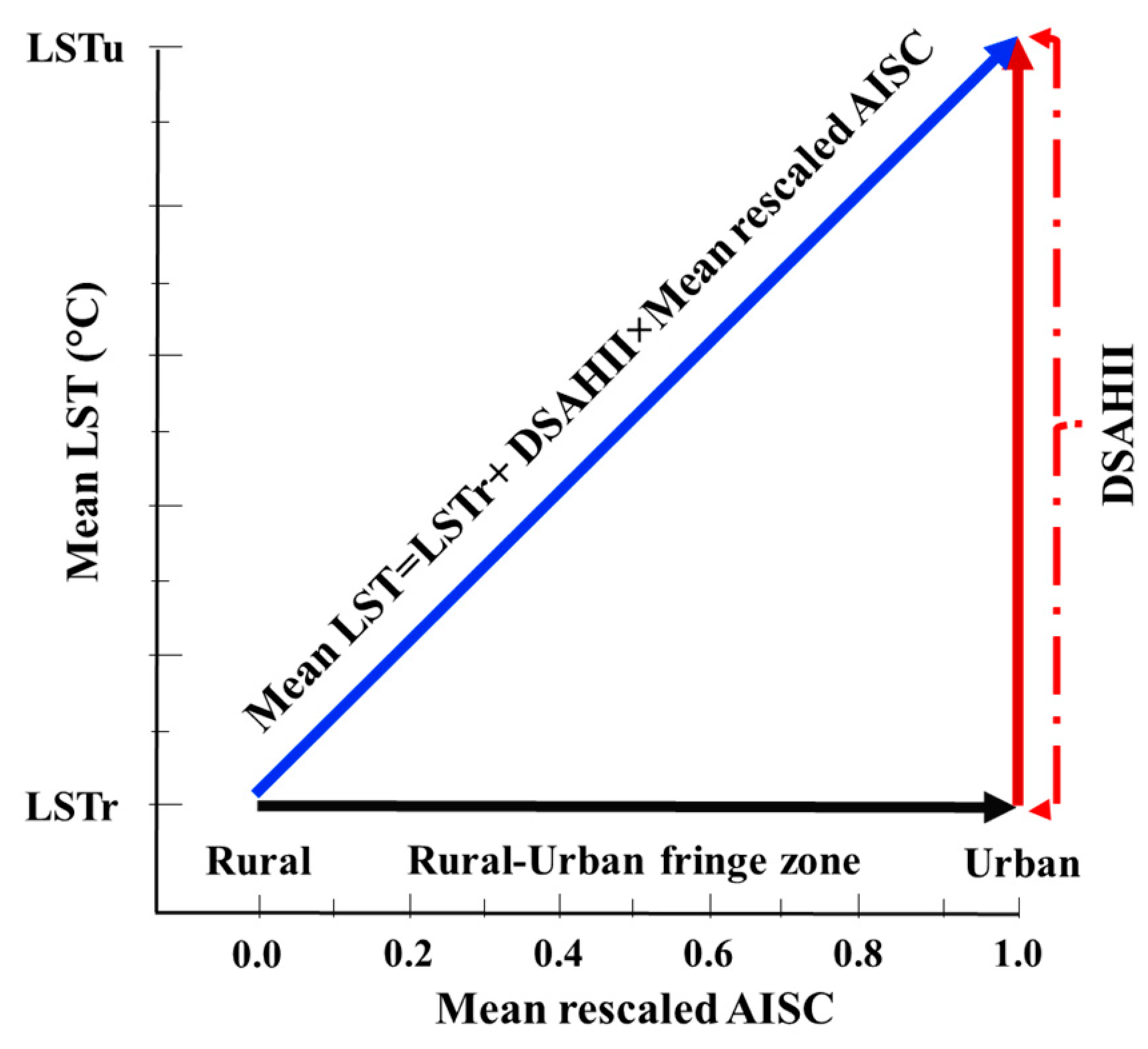
3.2.3. Quantifying DSAHII

Human activities such as the conversion of natural surfaces to urban surfaces are the most important factor affecting the change in SAHI. The conversion of natural surfaces into impervious urban lands increases the value of LST. ISC datasets such as HRLI and NLCD can be used to represent urban lands and human settlement regions [71,72]. In this study, HRLI and NLCD datasets were used to build the LST-AISC feature space (Figure 3). The fitted linear regression function slope, i.e., the increment of LST versus AISC, was used to quantify the DSAHII. The value of the slope indicates how much the LST value increases with increasing AISC. A higher slope value indicates a higher value of DSAHII. The process for DSAHII quantification is composed of the following four steps: (a) rescale the AISC values to between 0 and 1; (b) classify pixels based on the standardized AISC values per 100 classes with a class length of 0.01; (c) calculate the mean values of LST and rescale the AISC in each group of pixels to reduce the uncertainty caused by the heterogeneity of urban surfaces in modelling; (d) adapt an LLSM between the mean values of the LST and the rescaled AISC, in which the slope value of the fitted function indicates the value of the DSAHII. Additionally, the R2 value indicates the accuracy of the LLSM in DSAHII modelling.
In this study, the DSAHII values of different cities were calculated and compared based on the LLSM obtained from the LST-AISC feature space.

3.2.4. Evaluating the Efficiency of SIISC for DSAHII Quantification

To evaluate and compare the performance of the SIISC in DSAHII quantification, the SIISC was used instead of AISC in the conceptual model presented in Figure 3. The SIISC parameters include UI, BI, BAEM, BU, NBBSI, SI, IBI, albedo, NDBI, brightness, ABEI, and BCI. A DSAHII value was modelled for each city based on each spectral index. To evaluate the performance of the spectral indices in DSAHII quantification, the R2 and RMSE between the modelled DSAHII based on SIISC and the actual DSAHII obtained from the AISC were calculated.

4. Results

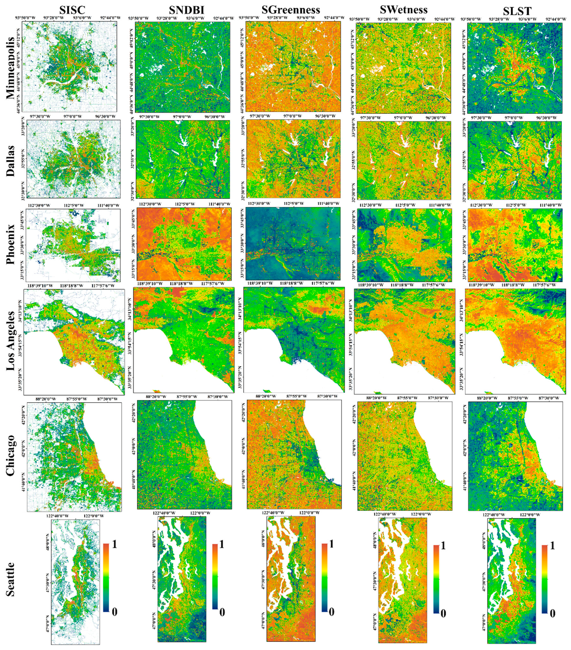
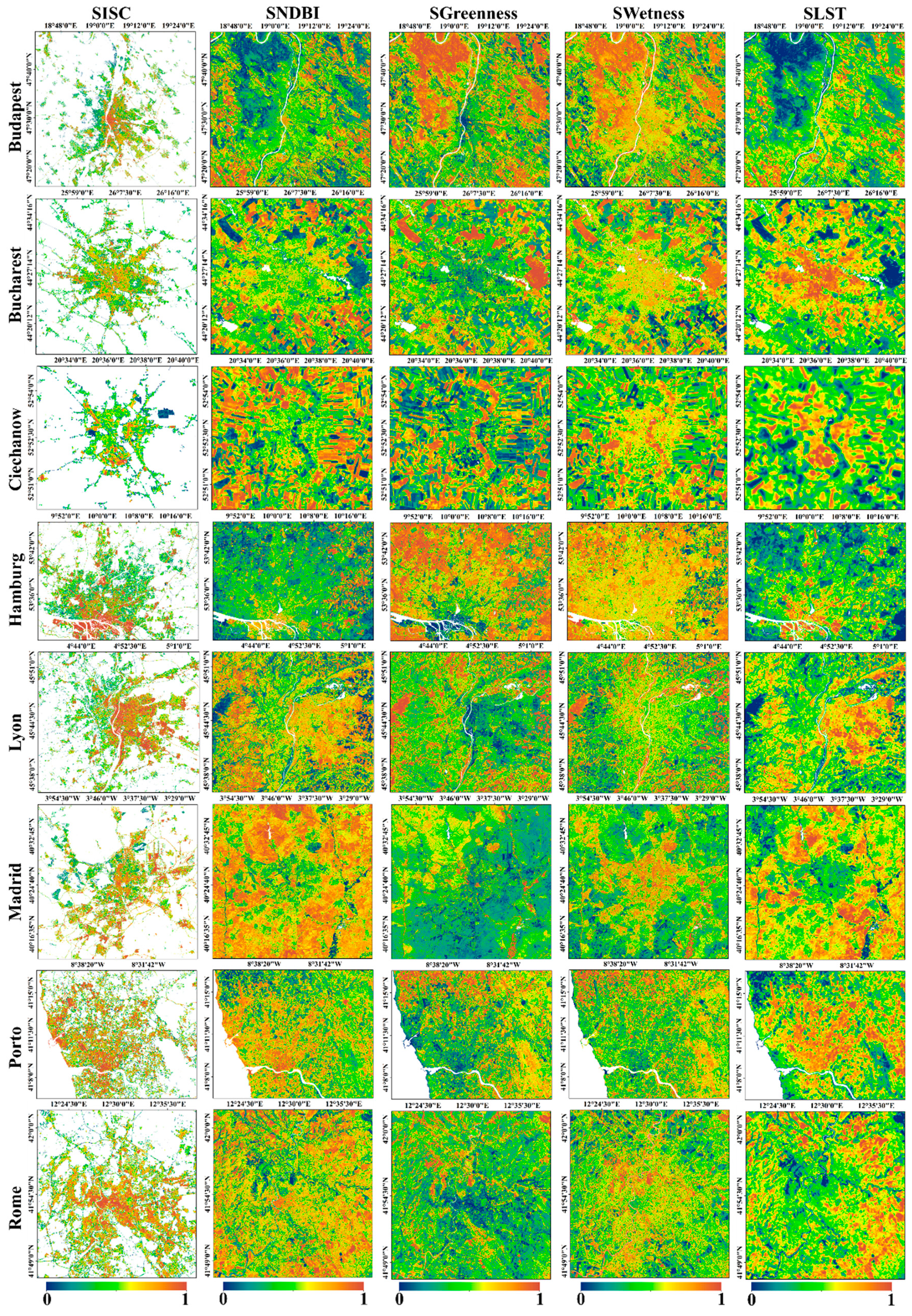
4.1. Spatial Distribution of Spectral Index Values

The mean values of R2 and RMSE between the LST values obtained from the Landsat 8 images and MOD11A1 for the selected cities were obtained to be 0.91 and 1.58 °C, respectively. These values indicate a reasonable accuracy of the Landsat 8-derived LST for these cities [2,73]. The spectral index values of selected cities were spatially heterogeneous (Figure 4 and Figure 5). The values of built-up land indices, BCI-derived characteristics, and LST in the central areas of the cities were higher than those in the suburbs.
The mean and SD values of the different spectral index values for the selected cities were different (Table 5). The mean (SD) values of the standardized LST (SLST) for European cities, namely, Budapest, Bucharest, Ciechanow, Hamburg, Lion, Madrid, Porto, and Rome, were 0.42 (0.10), 0.46 (0.11), 0.36 (0.11), 0.43 (0.08), 0.54 (0.09), 0.61 (0.10), 0.48 (0.17), and 0.45 (0.10), respectively. These values for the American cities, namely, Dallas, Seattle, Minneapolis, Los Angeles, Chicago, and Phoenix, were 0.50 (0.07), 0.39 (0.13), 0.33 (0.08), 0.42 (0.19), 0.43 (0.08), and 0.81 (0.08), respectively. Among European cities, the lowest and highest CV for SLST belonged to Madrid (0.16) and Porto (0.35), and among USA cities, belonged to Phoenix (0.09) and Los Angeles (0.45). The highest and lowest mean values of standardized AISC (SAISC) for the selected cities were found in Porto (0.66) and Seattle (0.37), respectively. The CVs of SAISC were 0.51, 0.45, 0.51, 0.45, 0.37, 0.39, 0.39, and 0.35 for the European cities, respectively, and 0.68, 0.70, 0.77, 0.50, 0.60, and 0.63 for the American cities, respectively. In general, the spatial variation of AISC was higher in USA cities than in European cities. Among the various indices, AISC and ABEI had the highest and lowest CV, respectively.

4.2. Quantifying DSAHII

The LST-AISC feature space formed for the different cities is shown in Figure 6. The results indicated that the mean LST values of suburban areas for the European cities, namely, Budapest, Bucharest, Ciechanow, Hamburg, Lyon, Madrid, Porto, and Rome, were 27.7, 29.8, 26.6, 24.3, 25.7, 31.2, 28.5, and 31.3 °C, respectively, and those for American cities, namely, Dallas, Seattle, Minneapolis, Los Angeles, Chicago, and Phoenix, were 30.4, 23.1, 27.6, 34.9, 27.2, and 40.8 °C, respectively. Rome and Madrid in Europe and Los Angeles and Phoenix in the USA have warmer and drier climates than the other cities, so their LSTs were higher than those of other cities. The R2 values between the mean values of LST and the rescaled AISC for the selected European cities were 0.98, 0.94, 0.93, 0.98, 0.98, 0.97, 0.98, and 0.96, respectively. For USA cities, these values were 0.97, 0.96, 0.98, 0.96, 0.95, and 0.94, respectively. These results indicate that the accuracy of the LLSM for DSAHII estimation is reasonably high.
The mean DSAHII values for selected European cities were 4.5, 6.6, 4.3, 3.5, 3.0, 3.0, 2.3, and 1.9 °C, respectively, and those for USA cities were 3.0, 6.7, 5.6, 4.4, 5.4, and 1.9 °C, respectively. The impact of human activity on LST varied among the selected cities. Among those, Rome and Seattle had the highest and lowest negative impacts of human activities on LST, respectively. The mean DSAHII values for the selected cities in Europe and USA were 3.6 and 4.5 °C, respectively. Generally, in green cities (with large fraction of vegetation coverage) including Hamburg, Budapest, Porto, Bucharest, Minneapolis, Seattle, Chicago, and Dallas due to high surface wetness and vegetation cover, and low heat and dryness, DSAHII is more intense. While in desert cities including Ciechanow, Madrid, Lyon, Rome, Los Angeles, and Phoenix, the DSAHII is lower.

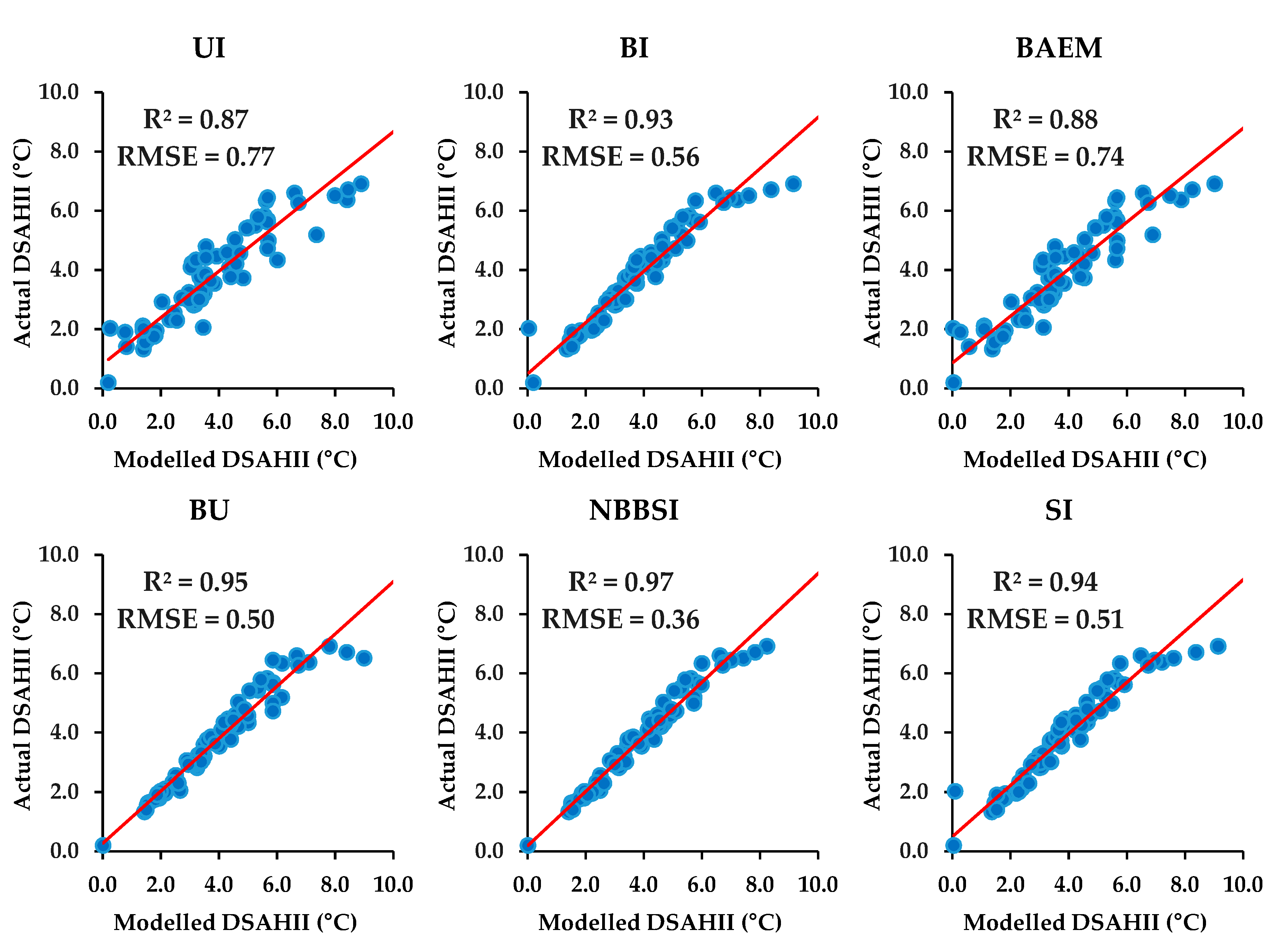
4.3. Evaluating the Effectiveness of SIISC for DSAHII Quantification

The performance of the SIISC parameters in DSAHII quantification differed (Figure 7). The obtained R2 values between the actual and modelled DSAHII based on UI, BI, BAEM, BU, NBBSI, SI, IBI, albedo, NDBI, brightness, ABEI, and BCI were 0.87, 0.93, 0.88, 0.95, 0.97, 0.94, 0.98, 0.76, 0.87, 0.52, 0.75, and 0.95, respectively. Additionally, the RMSE values between the actual and modelled DSAHII based on spectral index indicators were 0.77, 0.56, 0.74, 0.50, 0.36, 0.51, 0.34, 1.32, 0.74, 1.56, 1.58, and 0.83 °C, respectively. The IBI (R2 = 0.98, RMSE = 0.34 °C) had the highest performance in DSAHII quantification, but the performance of albedo (0.76, 1.32 °C), ABEI (0.75, 1.58 °C), and brightness (0.52, 1.52 °C) was poor. Our results show that the use of spectral indices such as IBI, BU, and NBBSI is quite useful and effective for DSAHII quantification.

5. Discussion

SAHIs are one of the important negative effects of human activity in the natural environment [37,48]. Increasing human activity increases the percentage of impermeable surfaces and increases the LST of these areas compared to that in natural areas (Figure 4 and Figure 5).
Marando, et al. [74] investigated the effect of green infrastructure elements such as urban and peri-urban forests, street trees, as well as the effect of vegetation cover and tree diversity in the reduction of the SUHI effect in Rome, Italy. The results of this study show that the green infrastructure significantly reduces the SUHI phenomenon in a Mediterranean city. Grigoraș and Urițescu [75] conducted an analysis based on multi-time remote sensing data to investigate the impact of land use change in Bucharest’s SUHI. The results suggest that the increase in built-up lands and the decrease in vegetation cover due to anthropogenic activities caused an increase in surface temperature and expansion of the area affected by SUHI. Arnds, et al. [76] analyzed the spatio-temporal variance of the SUHI of Hamburg. In summary, the SUHI showed a radial gradient in the center, which is mostly corresponding to the urban densities. Dian, et al. [77] studied the relationship between SUHII and local climate zones (LCZ) classes for Budapest. The results of this investigation indicate that as the density of the building decreases, the intensity of SUHI also decreases. The highest SUHII is in the city center and the lowest intensity of SUHI with negative values can be found in vegetation-covered LCZ classes.
Due to the negative consequences of the SAHI effect on various aspects of human quality of life, its quantification is of great importance. Firozjaei, Weng, Zhao, Kiavarz, Lu and Alavipanah [48] used a triple-SEB to model SAHII. The results showed that the triple-SEB could be highly effective for SAHII modelling. However, triple-SEBs are highly complex and require many calculations. Additionally, the implementation of this model requires many input datasets, including land cover parameters, surface digital models, climatic conditions, and so on.
Various studies have shown that ISC information is a good index for the degree of urban-related human activity in an area [38,41,43,44]. Zhang and Cheng [72] and Li, Zhou, Li, Meng, Wang, Wu and Sodoudi [71] used the LST-ISC feature space to model SUHII. The most important challenge of this method is using appropriate ISC information. Existing ISC databases have serious drawbacks, including spatial and temporal coverage constraints. However, satellite imagery can be used to address these challenges. In previous studies, various spectral indices and methods have been proposed for ISC modelling and built-up land extraction [51,53,61].
The results of this study showed that the IBI, BU, and NBBSI indices show good performance in DSAHII modelling (Figure 7). The TCT-derived brightness did not perform well in DSAHII modelling. Combining brightness with greenness and wetness information in the BCI increases the accuracy of DSAHII modelling. Some studies have shown that BCI can be effective in demonstrating spatial changes in the ISC in urban environments [24,70]. Firozjaei, Sedighi, Kiavarz, Qureshi, Haase and Alavipanah [61] showed that the ABEI is more effective than other indices for separating built-up lands from other land covers, especially bare lands. However, in this study, the ABEI accuracy for DSAHII quantification was lower than that of other indices. Therefore, this study showed that the ABEI is not suitable for heterogeneous modelling within built-up lands.
In general, SIISC has advantages for quantifying DSAHII, such as concurrency with thermal data recording, simplicity, low cost, accessibility under different spatial and temporal conditions, and scalability. The results showed that the use of the LST-SIISC feature space was highly effective for DSAHII modelling. However, one of the limitations of this method is that it is unable to model DSAHII changes in different geographical locations within a city. Therefore, to increase the spatial resolution of the modelled DSAHII, the LST-SIISC feature space must be implemented locally, such as for different urban regions.

6. Conclusions

SAHI modelling and quantification are very important to the quality of urban life. In this study, to evaluate and compare spectral indices used for DSAHII modelling, 14 cities in Europe and the USA with different conditions were selected. The DSAHII was quantified using the LST-AISC feature space and the LST-SIISC feature space. The results showed that the DSAHII in the selected cities in Europe and the USA was different. The DSAHII in cities with humid climates was higher than that in cities with dry climates. The performance of the spectral indices in DSAHII quantification varied. The results showed that IBI had the best performance for DSAHII quantification. In general, regarding the advantages of SIISC, it can be useful in identifying and characterizing the effects of human activity on the urban environment. It is suggested that in future studies, based on the approach presented in this study, the DSAHII in cities worldwide should be examined multi-temporally. Providing an appropriate model for future DSAHII prediction is also an important area for future studies.

Author Contributions

M.K.F., S.F., and N.M. conceived and designed the research of the first draft, and wrote the first draft; M.K., S.Q., S.K.A., and M.H. redesigned the research, revised and edited the paper. All authors have read and agreed to the published version of the manuscript.

Funding

This research received no external funding.

Acknowledgments

This study was supported by the Agrohydrology Research Group of Tarbiat Modares University (Grant No. IG-39713). We acknowledge support by the Open Access Publication Fund of Humboldt-Universität zu Berlin.

Conflicts of Interest

The authors declare no conflict of interest.

References

  1. Fu, P.; Weng, Q. A time series analysis of urbanization induced land use and land cover change and its impact on land surface temperature with Landsat imagery. Remote Sens. Environ. 2016, 175, 205–214. [Google Scholar] [CrossRef]
  2. Weng, Q.; Firozjaei, M.K.; Sedighi, A.; Kiavarz, M.; Alavipanah, S.K. Statistical analysis of surface urban heat island intensity variations: A case study of Babol city, Iran. Gisci. Remote Sens. 2019, 56, 576–604. [Google Scholar] [CrossRef]
  3. Fu, Y.; Li, J.; Weng, Q.; Zheng, Q.; Li, L.; Dai, S.; Guo, B. Characterizing the spatial pattern of annual urban growth by using time series Landsat imagery. Sci. Total Environ. 2019, 666, 274–284. [Google Scholar] [CrossRef] [PubMed]
  4. Mijani, N.; Alavipanah, S.K.; Firozjaei, M.K.; Arsanjani, J.J.; Hamzeh, S.; Weng, Q. Modeling outdoor thermal comfort using satellite imagery: A principle component analysis-based approach. Ecol. Indic. 2020, 117, 106555. [Google Scholar] [CrossRef]
  5. Firozjaei, M.K.; Kiavarz, M.; Alavipanah, S.K.; Lakes, T.; Qureshi, S. Monitoring and forecasting heat island intensity through multi-temporal image analysis and cellular automata-Markov chain modelling: A case of Babol city, Iran. Ecol. Indic. 2018, 91, 155–170. [Google Scholar] [CrossRef]
  6. Shahmohamadi, P.; Che-Ani, A.; Maulud, K.; Tawil, N.; Abdullah, N. The impact of anthropogenic heat on formation of urban heat island and energy consumption balance. Urban Stud. Res. 2011, 2011. [Google Scholar] [CrossRef] [Green Version]
  7. Haashemi, S.; Weng, Q.; Darvishi, A.; Alavipanah, S.K. Seasonal variations of the surface urban heat island in a semi-arid city. Remote Sens. 2016, 8, 352. [Google Scholar] [CrossRef] [Green Version]
  8. Liu, X.; Zhou, Y.; Yue, W.; Li, X.; Liu, Y.; Lu, D. Spatiotemporal patterns of summer urban heat island in Beijing, China using an improved land surface temperature. J. Clean. Prod. 2020, 257, 120529. [Google Scholar] [CrossRef]
  9. Voogt, J.A.; Oke, T.R. Thermal remote sensing of urban climates. Remote Sens Environ. 2003, 86, 370–384. [Google Scholar] [CrossRef]
  10. Howard, L. The Climate of London: Deduced from Meteorological Observations Made in the Metropolis and at Various Places Around it Vols. I–III; Harvard University: Cambridge, MA, USA, 1833. [Google Scholar]
  11. Knapp, S.; Kühn, I.; Stolle, J.; Klotz, S. Changes in the functional composition of a Central European urban flora over three centuries. Perspect. Plant Ecol. Evol. Syst. 2010, 12, 235–244. [Google Scholar] [CrossRef]
  12. Gaur, A.; Eichenbaum, M.K.; Simonovic, S.P. Analysis and modelling of surface Urban Heat Island in 20 Canadian cities under climate and land-cover change. J. Environ. Manag. 2018, 206, 145–157. [Google Scholar] [CrossRef] [PubMed]
  13. Li, H.; Meier, F.; Lee, X.; Chakraborty, T.; Liu, J.; Schaap, M.; Sodoudi, S. Interaction between urban heat island and urban pollution island during summer in Berlin. Sci. Total Environ. 2018, 636, 818–828. [Google Scholar] [CrossRef] [PubMed]
  14. Guattari, C.; Evangelisti, L.; Balaras, C.A. On the assessment of urban heat island phenomenon and its effects on building energy performance: A case study of Rome (Italy). Energy Build. 2018, 158, 605–615. [Google Scholar] [CrossRef]
  15. Zheng, Z.; Ren, G.; Wang, H.; Dou, J.; Gao, Z.; Duan, C.; Li, Y.; Ngarukiyimana, J.P.; Zhao, C.; Cao, C. Relationship between fine-particle pollution and the urban heat island in Beijing, China: Observational evidence. Bound. -Layer Meteorol. 2018, 169, 93–113. [Google Scholar] [CrossRef]
  16. Zhao, L.; Oppenheimer, M.; Zhu, Q.; Baldwin, J.W.; Ebi, K.L.; Bou-Zeid, E.; Guan, K.; Liu, X. Interactions between urban heat islands and heat waves. Environ. Res. Lett. 2018, 13, 034003. [Google Scholar] [CrossRef]
  17. Li, X.; Li, W.; Middel, A.; Harlan, S.; Brazel, A.; Turner, B. Remote sensing of the surface urban heat island and land architecture in Phoenix, Arizona: Combined effects of land composition and configuration and cadastral–demographic–economic factors. Remote Sens. Environ. 2016, 174, 233–243. [Google Scholar] [CrossRef] [Green Version]
  18. Taleghani, M. Outdoor thermal comfort by different heat mitigation strategies-A review. Renew. Sustain. Energy Rev. 2018, 81, 2011–2018. [Google Scholar] [CrossRef]
  19. Watkins, R.; Palmer, J.; Kolokotroni, M. Increased temperature and intensification of the urban heat island: Implications for human comfort and urban design. Built Environ. 2007, 33, 85–96. [Google Scholar] [CrossRef]
  20. Kolokotroni, M.; Ren, X.; Davies, M.; Mavrogianni, A. London’s urban heat island: Impact on current and future energy consumption in office buildings. Energy Build. 2012, 47, 302–311. [Google Scholar] [CrossRef] [Green Version]
  21. Herbel, I.; Croitoru, A.-E.; Rus, A.V.; Roşca, C.F.; Harpa, G.V.; Ciupertea, A.-F.; Rus, I. The impact of heat waves on surface urban heat island and local economy in Cluj-Napoca city, Romania. Theor. Appl. Climatol. 2018, 133, 681–695. [Google Scholar] [CrossRef]
  22. Shen, H.; Huang, L.; Zhang, L.; Wu, P.; Zeng, C. Long-term and fine-scale satellite monitoring of the urban heat island effect by the fusion of multi-temporal and multi-sensor remote sensed data: A 26-year case study of the city of Wuhan in China. Remote Sens. Environ. 2016, 172, 109–125. [Google Scholar] [CrossRef]
  23. He, X.; Wang, J.; Feng, J.; Yan, Z.; Miao, S.; Zhang, Y.; Xia, J. Observational and modeling study of interactions between urban heat island and heatwave in Beijing. J. Clean. Prod. 2020, 247, 119169. [Google Scholar] [CrossRef]
  24. Meng, Q.; Zhang, L.; Sun, Z.; Meng, F.; Wang, L.; Sun, Y. Characterizing spatial and temporal trends of surface urban heat island effect in an urban main built-up area: A 12-year case study in Beijing, China. Remote Sens. Environ. 2018, 204, 826–837. [Google Scholar] [CrossRef]
  25. Zhou, D.; Zhao, S.; Liu, S.; Zhang, L.; Zhu, C. Surface urban heat island in China’s 32 major cities: Spatial patterns and drivers. Remote Sens. Environ. 2014, 152, 51–61. [Google Scholar] [CrossRef]
  26. Liu, N.; Morawska, L. Modeling the urban heat island mitigation effect of cool coatings in realistic urban morphology. J. Clean. Prod. 2020, 121560. [Google Scholar] [CrossRef]
  27. Sun, R.; Lü, Y.; Yang, X.; Chen, L. Understanding the variability of urban heat islands from local background climate and urbanization. J. Clean. Prod. 2019, 208, 743–752. [Google Scholar] [CrossRef]
  28. Schwarz, N.; Lautenbach, S.; Seppelt, R. Exploring indicators for quantifying surface urban heat islands of European cities with MODIS land surface temperatures. Remote Sens. Environ. 2011, 115, 3175–3186. [Google Scholar] [CrossRef]
  29. Weng, Q. Thermal infrared remote sensing for urban climate and environmental studies: Methods, applications, and trends. ISPRS J. Photogramm. 2009, 64, 335–344. [Google Scholar] [CrossRef]
  30. Oke, T.R. The energetic basis of the urban heat island. Q. J. R. Meteorol. Soc. 1982, 108, 1–24. [Google Scholar] [CrossRef]
  31. Firozjaei, M.K.; Fathololoumi, S.; Kiavarz, M.; Arsanjani, J.J.; Alavipanah, S.K. Modelling surface heat island intensity according to differences of biophysical characteristics: A case study of Amol city, Iran. Ecol. Indic. 2020, 109, 105816. [Google Scholar] [CrossRef]
  32. Alavipanah, S.; Schreyer, J.; Haase, D.; Lakes, T.; Qureshi, S. The effect of multi-dimensional indicators on urban thermal conditions. J. Clean. Prod. 2018, 177, 115–123. [Google Scholar] [CrossRef]
  33. Leal Filho, W.; Icaza, L.E.; Neht, A.; Klavins, M.; Morgan, E.A. Coping with the impacts of urban heat islands. A literature based study on understanding urban heat vulnerability and the need for resilience in cities in a global climate change context. J. Clean. Prod. 2018, 171, 1140–1149. [Google Scholar] [CrossRef] [Green Version]
  34. Gartland, L.M. Heat Islands: Understanding and Mitigating Heat in Urban Areas; Routledge: Abingdon-on-Thames, UK, 2012. [Google Scholar]
  35. Zhang, Y.; Balzter, H.; Wu, X. Spatial–temporal patterns of urban anthropogenic heat discharge in Fuzhou, China, observed from sensible heat flux using Landsat TM/ETM+ data. Int. J. Remote Sens. 2013, 34, 1459–1477. [Google Scholar] [CrossRef] [Green Version]
  36. Kato, S.; Yamaguchi, Y. Analysis of urban heat-island effect using ASTER and ETM+ Data: Separation of anthropogenic heat discharge and natural heat radiation from sensible heat flux. Remote Sens. Environ. 2005, 99, 44–54. [Google Scholar] [CrossRef]
  37. Chen, S.; Hu, D.; Wong, M.S.; Ren, H.; Cao, S.; Yu, C.; Ho, H.C. Characterizing spatiotemporal dynamics of anthropogenic heat fluxes: A 20-year case study in Beijing–Tianjin–Hebei region in China. Environ. Pollut. 2019, 249, 923–931. [Google Scholar] [CrossRef] [PubMed]
  38. Wang, S.; Hu, D.; Chen, S.; Yu, C. A Partition Modeling for Anthropogenic Heat Flux Mapping in China. Remote Sens. 2019, 11, 1132. [Google Scholar] [CrossRef] [Green Version]
  39. Sun, R.; Wang, Y.; Chen, L. A distributed model for quantifying temporal-spatial patterns of anthropogenic heat based on energy consumption. J. Clean. Prod. 2018, 170, 601–609. [Google Scholar] [CrossRef]
  40. Iamarino, M.; Beevers, S.; Grimmond, C. High-resolution (space, time) anthropogenic heat emissions: London 1970–2025. Int. J. Climatol. 2012, 32, 1754–1767. [Google Scholar] [CrossRef] [Green Version]
  41. Chen, S.; Hu, D. Parameterizing Anthropogenic Heat Flux with an Energy-Consumption Inventory and Multi-Source Remote Sensing Data. Remote Sens. 2017, 9, 1165. [Google Scholar] [CrossRef] [Green Version]
  42. Hu, D.; Yang, L.; Zhou, J.; Deng, L. Estimation of urban energy heat flux and anthropogenic heat discharge using aster image and meteorological data: Case study in Beijing metropolitan area. J. Appl. Remote Sens. 2012, 6, 063559. [Google Scholar] [CrossRef]
  43. Fu, P.; Weng, Q. Responses of urban heat island in Atlanta to different land-use scenarios. Theor. Appl. Climatol. 2018, 133, 123–135. [Google Scholar] [CrossRef]
  44. Gabey, A.; Grimmond, C.; Capel-Timms, I. Anthropogenic heat flux: Advisable spatial resolutions when input data are scarce. Theor. Appl. Climatol. 2019, 135, 791–807. [Google Scholar] [CrossRef] [Green Version]
  45. Liu, K.; Fang, J.-y.; Zhao, D.; Liu, X.; Zhang, X.-h.; Wang, X.; Li, X.-k. An assessment of urban surface energy fluxes using a sub-pixel remote sensing analysis: A case study in Suzhou, China. ISPRS Int. J. Geo-Inf. 2016, 5, 11. [Google Scholar] [CrossRef]
  46. Zhou, J.; Hu, D.; Weng, Q. Analysis of surface radiation budget during the summer and winter in the metropolitan area of Beijing, China. J. Appl. Remote Sens. 2010, 4, 043513. [Google Scholar]
  47. Weng, Q.; Hu, X.; Quattrochi, D.A.; Liu, H. Assessing intra-urban surface energy fluxes using remotely sensed ASTER imagery and routine meteorological data: A case study in Indianapolis, USA. IEEE J. Sel. Top. Appl. Earth Obs. Remote Sens. 2014, 7, 4046–4057. [Google Scholar] [CrossRef]
  48. Firozjaei, M.K.; Weng, Q.; Zhao, C.; Kiavarz, M.; Lu, L.; Alavipanah, S.K. Surface anthropogenic heat islands in six megacities: An assessment based on a triple-source surface energy balance model. Remote Sens. Environ. 2020, 242, 111751. [Google Scholar] [CrossRef]
  49. Kawamura, M.; Jayamana, S.; Tsujiko, Y. Relation between social and environmental conditions in Colombo Sri Lanka and the urban index estimated by satellite remote sensing data. Int. Arch. Photogramm. Remote Sens. 1996, 31, 321–326. [Google Scholar]
  50. Zhao, H.; Chen, X. Use of normalized difference bareness index in quickly mapping bare areas from TM/ETM+. Int. Geosci. Remote Sens. Symp. 2005, 3, 1666. [Google Scholar]
  51. Zha, Y.; Gao, J.; Ni, S. Use of normalized difference built-up index in automatically mapping urban areas from TM imagery. Int. J. Remote Sens. 2003, 24, 583–594. [Google Scholar] [CrossRef]
  52. Xu, H. A new index for delineating built-up land features in satellite imagery. Int. J. Remote Sens. 2008, 29, 4269–4276. [Google Scholar] [CrossRef]
  53. He, C.; Shi, P.; Xie, D.; Zhao, Y. Improving the normalized difference built-up index to map urban built-up areas using a semiautomatic segmentation approach. Remote Sens. Lett. 2010, 1, 213–221. [Google Scholar] [CrossRef] [Green Version]
  54. Waqar, M.M.; Mirza, J.F.; Mumtaz, R.; Hussain, E. Development of new indices for extraction of built-up area & bare soil from landsat data. Open Access Sci. Rep 2012, 1, 4. [Google Scholar]
  55. Kaimaris, D.; Patias, P. Identification and area measurement of the built-up area with the Built-up Index (BUI). Int. J. Adv. Remote Sens. Gis 2016, 5, 1844–1858. [Google Scholar] [CrossRef] [Green Version]
  56. Bouzekri, S.; Lasbet, A.A.; Lachehab, A. A new spectral index for extraction of built-up area using landsat-8 data. J. Indian Soc. Remote Sens. 2015, 43, 867–873. [Google Scholar] [CrossRef]
  57. Rikimaru, A. Development of forest canopy density mapping and monitoring model using indices of vegetation, bare soil and shadow. In Presented Paper. 18th ACRS; Hosei University: Tokyo, Japan, 1997. [Google Scholar]
  58. Yang, C.; Zhang, C.; Li, Q.; Liu, H.; Gao, W.; Shi, T.; Liu, X.; Wu, G. Rapid urbanization and policy variation greatly drive ecological quality evolution in Guangdong-Hong Kong-Macau Greater Bay Area of China: A remote sensing perspective. Ecol. Indic. 2020, 115, 106373. [Google Scholar] [CrossRef]
  59. Bhatti, S.S.; Tripathi, N.K. Built-up area extraction using Landsat 8 OLI imagery. Gisci. Remote Sens. 2014, 51, 445–467. [Google Scholar] [CrossRef] [Green Version]
  60. As-syakur, A.; Adnyana, I.; Arthana, I.W.; Nuarsa, I.W. Enhanced built-up and bareness index (EBBI) for mapping built-up and bare land in an urban area. Remote Sens. 2012, 4, 2957–2970. [Google Scholar] [CrossRef] [Green Version]
  61. Firozjaei, M.K.; Sedighi, A.; Kiavarz, M.; Qureshi, S.; Haase, D.; Alavipanah, S.K. Automated Built-Up Extraction Index: A New Technique for Mapping Surface Built-Up Areas Using LANDSAT 8 OLI Imagery. Remote Sens. 2019, 11, 1966. [Google Scholar] [CrossRef] [Green Version]
  62. Firozjaei, M.K.; Fathololoumi, S.; Weng, Q.; Kiavarz, M.; Alavipanah, S.K. Remotely Sensed Urban Surface Ecological Index (RSUSEI): An Analytical Framework for Assessing the Surface Ecological Status in Urban Environments. Remote Sens. 2020, 12, 2029. [Google Scholar] [CrossRef]
  63. Ding, H.; Shi, W. Land-use/land-cover change and its influence on surface temperature: A case study in Beijing City. Int. J. Remote Sens. 2013, 34, 5503–5517. [Google Scholar] [CrossRef]
  64. Boori, M.S. A comparison of land surface temperature, derived from AMSR-2, Landsat and ASTER satellite data. J. Geogr. Geol. 2015, 7, 61. [Google Scholar] [CrossRef]
  65. Berk, A.; Conforti, P.; Kennett, R.; Perkins, T.; Hawes, F.; van den Bosch, J. MODTRAN® 6: A major upgrade of the MODTRAN® radiative transfer code. In Proceedings of the Hyperspectral Image and Signal Processing: Evolution in Remote Sensing (WHISPERS), Lausanne, Switzerland, 24–27 June 2014; pp. 1–4. [Google Scholar]
  66. Jimenez-Munoz, J.C.; Sobrino, J.A.; Skokovic, D.; Mattar, C.; Cristobal, J. Land Surface Temperature Retrieval Methods From Landsat-8 Thermal Infrared Sensor Data. IEEE Geosci. Remote Sens. 2014, 11, 1840–1843. [Google Scholar] [CrossRef]
  67. Montanaro, M.; Gerace, A.; Lunsford, A.; Reuter, D. Stray light artifacts in imagery from the Landsat 8 Thermal Infrared Sensor. Remote Sens. 2014, 6, 10435–10456. [Google Scholar] [CrossRef] [Green Version]
  68. Duan, S.-B.; Li, Z.-L.; Wang, C.; Zhang, S.; Tang, B.-H.; Leng, P.; Gao, M.-F. Land-surface temperature retrieval from Landsat 8 single-channel thermal infrared data in combination with NCEP reanalysis data and ASTER GED product. Int. J. Remote Sens. 2019, 40, 1763–1778. [Google Scholar] [CrossRef]
  69. Mijani, N.; Alavipanah, S.K.; Hamzeh, S.; Firozjaei, M.K.; Arsanjani, J.J. Modeling thermal comfort in different condition of mind using satellite images: An Ordered Weighted Averaging approach and a case study. Ecol. Indic. 2019, 104, 1–12. [Google Scholar] [CrossRef]
  70. Deng, C.; Wu, C. BCI: A biophysical composition index for remote sensing of urban environments. Remote Sens. Environ. 2012, 127, 247–259. [Google Scholar] [CrossRef]
  71. Li, H.; Zhou, Y.; Li, X.; Meng, L.; Wang, X.; Wu, S.; Sodoudi, S. A new method to quantify surface urban heat island intensity. Sci. Total Environ. 2018, 624, 262–272. [Google Scholar] [CrossRef]
  72. Zhang, Y.; Cheng, J. Spatio-Temporal Analysis of Urban Heat Island Using Multisource Remote Sensing Data: A Case Study in Hangzhou, China. IEEE J. Sel. Top. Appl. Earth Obs. Remote Sens. 2019, 12, 3317–3326. [Google Scholar] [CrossRef]
  73. Firozjaei, M.K.; Alavipanah, S.K.; Liu, H.; Sedighi, A.; Mijani, N.; Kiavarz, M.; Weng, Q. A PCA–OLS Model for Assessing the Impact of Surface Biophysical Parameters on Land Surface Temperature Variations. Remote Sens. 2019, 11, 2094. [Google Scholar] [CrossRef] [Green Version]
  74. Marando, F.; Salvatori, E.; Sebastiani, A.; Fusaro, L.; Manes, F. Regulating ecosystem services and green infrastructure: Assessment of urban heat island effect mitigation in the municipality of Rome, Italy. Ecol. Model. 2019, 392, 92–102. [Google Scholar] [CrossRef]
  75. Grigoraș, G.; Urițescu, B. Land Use/Land Cover Changes Dynamics and Their Effects on Surface Urban Heat Island in Bucharest, Romania. Int. J. Appl. Earth Obs. Geoinf. 2019, 80, 115–126. [Google Scholar] [CrossRef]
  76. Arnds, D.; Böhner, J.; Bechtel, B. Spatio-temporal variance and meteorological drivers of the urban heat island in a European city. Theor. Appl. Climatol. 2017, 128, 43–61. [Google Scholar] [CrossRef]
  77. Dian, C.; Pongrácz, R.; Dezső, Z.; Bartholy, J. Annual and monthly analysis of surface urban heat island intensity with respect to the local climate zones in Budapest. Urban Clim. 2020, 31, 100573. [Google Scholar] [CrossRef]
Figure 1. Geographical location and colour-composite images (Blue, near-infrared (NIR), and Short-wave infrared 2 (SWIR2) bands) of selected cities in the USA and Europe.
Remotesensing 12 02854 g001
Figure 2. Flowchart of the study.
Remotesensing 12 02854 g002
Figure 3. Conceptual diagram of modelling the daytime surface anthropogenic heat island intensity (DSAHII) based on the land surface temperature (LST)-actual impervious surface cover (AISC) feature space. The LSTu is the urban LST, representing the LST in the urban area where the rescaled AISC is 1 (AISC is 100%), and LSTr is the rural LST, representing the LST in the rural area where the rescaled AISC is 0 (AISC is 0%).
Remotesensing 12 02854 g003
Figure 4. The mean of standardized ISC (SISC), standardized normalized difference built-up index (SNDBI), standardized greenness (SGreeness), standardized wetness (SWetness), and standardized LST (SLST) maps for the selected cities in USA on different dates.
Remotesensing 12 02854 g004
Figure 5. The mean of SISC, SNDBI, SGreeness, SWetness, and SLST maps for selected cities in Europe on different dates.
Remotesensing 12 02854 g005
Figure 6. The mean value of DSAHII obtained from the LST-ISC feature space for selected cities in Europe and USA on different dates.
Remotesensing 12 02854 g006
Figure 7. The obtained R2 and root mean square error (RMSE) values between the actual and modelled DSAHII based on spectral index-based ISC (SIISC). Solid red line represents the predicted relationship between actual and modeled DSAHII.
Remotesensing 12 02854 g007aRemotesensing 12 02854 g007b
Table 1. Summary characteristics of selected cities in the USA and Europe.
Centre Point Coordinate (Lon, Lat-WGS84)CountryArea (km2)Mean Alt. (m)ClimatePopulation (2020)
European cities
Rome12.45, 41.85 Italy631.750Mediterranean >4,250,000
Madrid−3.70, 40.41Spain2332.3650Mediterranean and semi-arid>6,670,000
Porto−8.60, 41.16Portugal481.480Mediterranean>1,309,000
Lyon4.83, 45.76 France1143.6175Humid subtropical>1,710,000
Ciechanow20.60, 52.82Poland81.1151Humid subtropical>44,000
Hamburg10.02, 53.60Germany1097.510Oceanic>1,795,000
Budapest19.07, 47.59Hungary3664.3120Oceanic and Humid subtropical>1,764,000
Bucharest26.10, 44.42Romania1385.785Humid continental>1,815,000
American cities
Minneapolis−93.26, 44.97United States8719.6253Humid continental>432,110
Fort Worth−96.95, 36.8514,998.1199Humid subtropical>875,000
Phoenix−112.09, 33.128543.8331Midlatitude desert>1,632,000
Seattle−122.25, 45.4711,497.552Marine West coast>3,406,000
Chicago−87.66, 41.8612,685.1182Humid continental>2,705,000
Los Angeles−118.22, 34.0011,127.4282Mediterranean>4,000,000
Table 2. Details of the data utilized in the study.
Landsat 8
Selected CitiesDateRowPathSpatial ResolutionSource
Rome12 April 2015,19103130 m for reflective and 100 m for thermal bandsUnited States Geological Survey (USGS) website
14 May 2015,
30 May 2015,
01 July 2015,
17 July 2015
Madrid02 April 2015,197028
20 May 2015,
21 June 2015,
07 July 2015,
23 July 2015,
25 September 2015
Porto07 April 2015,204032
16 May 2015,
17 June 2015,
03 July 2015,
12 July 2015,
28 July 2015,
04 August 2015,
29 August 2015,
21 September 2015
Lyon06 April 2015,196023
25 June 2015,
04 July 2015,
05 August 2015,
21 August 2015,
28 August 2015,
29 September 2015
Ciechanow23 April 2015,189023
03 July 2015,
04 August 2015,
13 August 2015
Hamburg15 April 2015,20134
24 April 2015,
11 June 2015,
04 July 2015,
21 August 2015
Budapest16 April 2015,188027
10 June 2015,
12 July 2015,
13 August 2015,
29 August 2015
Bucharest13 April 2015,182029
15 May 2015,
07 June 2015,
09 July 2015,
25 July 2015,
03 August 2015,
26 August 2015,
04 September 2015
Minneapolis19 May 2016,027029
20 June 2016,
06 July 2016,
22 July 2016,
23 August 2016,
08 September 2016
Dallas03 May 2016,027037
06 July 2016,
22 July 2016,
07 August 2016,
08 September 2016
Phoenix23 April 2016,037037
09 May 2016,
25 May 2016,
12 July 2016,
28 July 2016,
29 August 2016,
14 September 2016
Seattle31 May 2016,046027
27 July 2016,
03 August 2016,
12 August 2016,
19 August 2016,
13 September 2016
Chicago05 April 2016,021031
14 April 2016,
23 May 2016,
08 June 2016,
17 June 2016,
24 June 2016,
04 August 2016,
12 September 2016
Los Angeles19 April 2016,041037
22 June 2016,
08 July 2016,
24 July 2016,
09 August 2016,
25 August 2016,
10 September 2016,
26 September 2016
MODIS products
MOD07Landsat 8 overpass dates-5000 mAtmosphere Archive and Distribution System (AADS) website
MOD11A11000 m
AISC dataset
NLCD imperviousness2016-30 mUSGS at the https://www.mrlc.gov/data website
HRLI201520 mCopernicus Global Land Service (CGLS) at the https://land.copernicus.eu/ website
Table 3. Spectral and spatial characteristics of Landsat 8 bands.
Band NumbersBand NamesSensorEffective Wavelength (Micrometer)Spatial Resolution (Meter)
B1Coastal aerosolOLI0.44330
B2Blue0.4826
B3Green0.5613
B4Red0.6546
B5Near Infrared (NIR)0.8646
B6SWIR 11.609
B7SWIR 22.201
B8Panchromatic0.591715
B9Cirrus1.37330
B10Thermal Infrared 1TIRS10.9100 (resampled to 30)
B11Thermal Infrared 212.0
Table 4. Spectral indices used in this study.
Spectral IndexEquation
NDBI B 6 B 5 B 6 + B 5
BI ( B 6 + B 4 ) ( B 5 + B 2 ) ( B 6 + B 4 ) + ( B 5 + B 2 )
UI B 7 B 5 B 7 + B 5
IBI ( ( 2 B 6 B 6 + B 5 ) ( B 5 B 5 + B 4 ) + ( B 3 B 3 + B 6 ) ) / ( ( 2 B 6 B 6 + B 5 ) + ( B 5 B 5 + B 4 ) ( B 3 B 3 + B 6 ) )
BU NDBI NDVI
BAEM NDBI NDVI MNDWI
Albedo 0.2266 B 1 + 0.2320 B 2 0.2138 B 3 0.1803 B 4 + 0.1103 B 5 0.0278 B 6 + 0.0099 B 7
ABEI 0.312 B 1 + 0.513 B 2 0.086 B 3 0.441 B 4 + 0.052 B 5 0.198 B 6 + 0.278 B 7
SI ( B 6 + B 4 ) ( B 5 + B 2 ) / ( B 6 + B 4 ) + ( B 5 + B 2 )
NBBSI ( SI + IBI ) 2
Table 5. The mean value and SD of the different spectral index values for the selected cities on different dates. SISC: Standardized Impervious Surface Cover; SUI: Standardized Urban Index; SBI: Standardized Bare Soil Index; SBAEM: Standardized Built-up Area Extraction Method; SBU: Standardized Built-up Index; SBBSI: Standardized Built-up and Bare Soil Index; SSI: Standardized soil index (SI); SIBI: Standardized Index-based Built-up Index; SAlbedo: Standardized Albedo; SNDBI: Standardized Normalized Difference Built-up Index; SBrightness: Standardized Brightness; SABEI: Standardized Automated Built-up Extraction Index; SBCI: Standardized Biophysical Composition Index; SLST: Standardized Land Surface Temperature.
CitiesParametersSISCSUISBISBAEMSBUSBBSISSISIBISAlbedoSNDBISBrightnessSABEISBCISLST
BudapestMean0.410.710.340.680.590.620.340.740.140.010.010.320.160.42
SD0.210.050.110.050.070.080.110.050.060.010.010.060.070.10
BucharestMean0.510.640.360.630.500.510.360.510.130.010.010.270.170.46
SD0.230.020.070.030.030.050.070.030.020.000.000.010.030.11
CiechanowMean0.390.480.570.560.390.550.570.400.180.480.310.260.130.36
SD0.200.160.180.160.150.190.180.140.040.160.060.040.070.11
HamburgMean0.590.560.320.370.240.450.320.460.090.560.090.240.180.43
SD0.270.050.070.050.080.090.070.080.020.050.020.010.030.08
LyonMean0.650.500.570.570.500.660.570.520.130.500.110.260.200.54
SD0.240.080.040.070.090.060.040.060.020.080.020.010.030.09
MadridMean0.630.740.040.460.470.850.040.870.130.740.110.270.160.61
SD0.240.030.010.040.060.160.810.090.020.030.030.010.030.10
PortoMean0.660.310.850.390.350.080.850.870.180.310.130.280.200.48
SD0.260.070.310.090.090.470.310.280.040.070.060.010.060.17
RomeMean0.630.360.360.380.300.570.360.560.130.360.110.270.150.45
SD0.230.080.110.090.110.120.110.110.020.080.020.020.040.10
DallasMean0.450.350.130.310.200.060.130.190.140.350.130.250.190.50
SD0.290.020.010.020.030.010.010.020.030.020.040.020.030.07
SeattleMean0.370.310.310.370.230.370.310.370.070.310.090.320.180.39
SD0.260.110.150.10.120.150.150.190.040.110.050.010.060.13
MinneapolisMean0.360.340.310.450.170.320.310.240.040.340.080.190.220.33
SD0.280.070.090.070.080.130.090.130.010.070.020.010.020.08
Los AngelesMean0.560.540.440.530.560.560.440.560.10.540.10.350.260.42
SD0.260.090.130.110.10.090.130.140.060.090.060.040.060.19
ChicagoMean0.430.380.290.460.240.340.290.360.060.380.10.190.140.43
SD0.260.060.10.070.130.120.10.190.030.070.060.010.040.08
PhoenixMean0.410.50.580.580.380.640.580.470.10.510.150.270.180.81
SD0.260.060.080.070.060.090.080.070.030.060.040.010.040.08

