Investigations into Synoptic Spatiotemporal Characteristics of Coastal Upper Ocean Circulation Using High Frequency Radar Data and Model Output


Abstract
:
1. Introduction
2. Methodologies
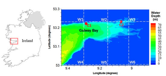
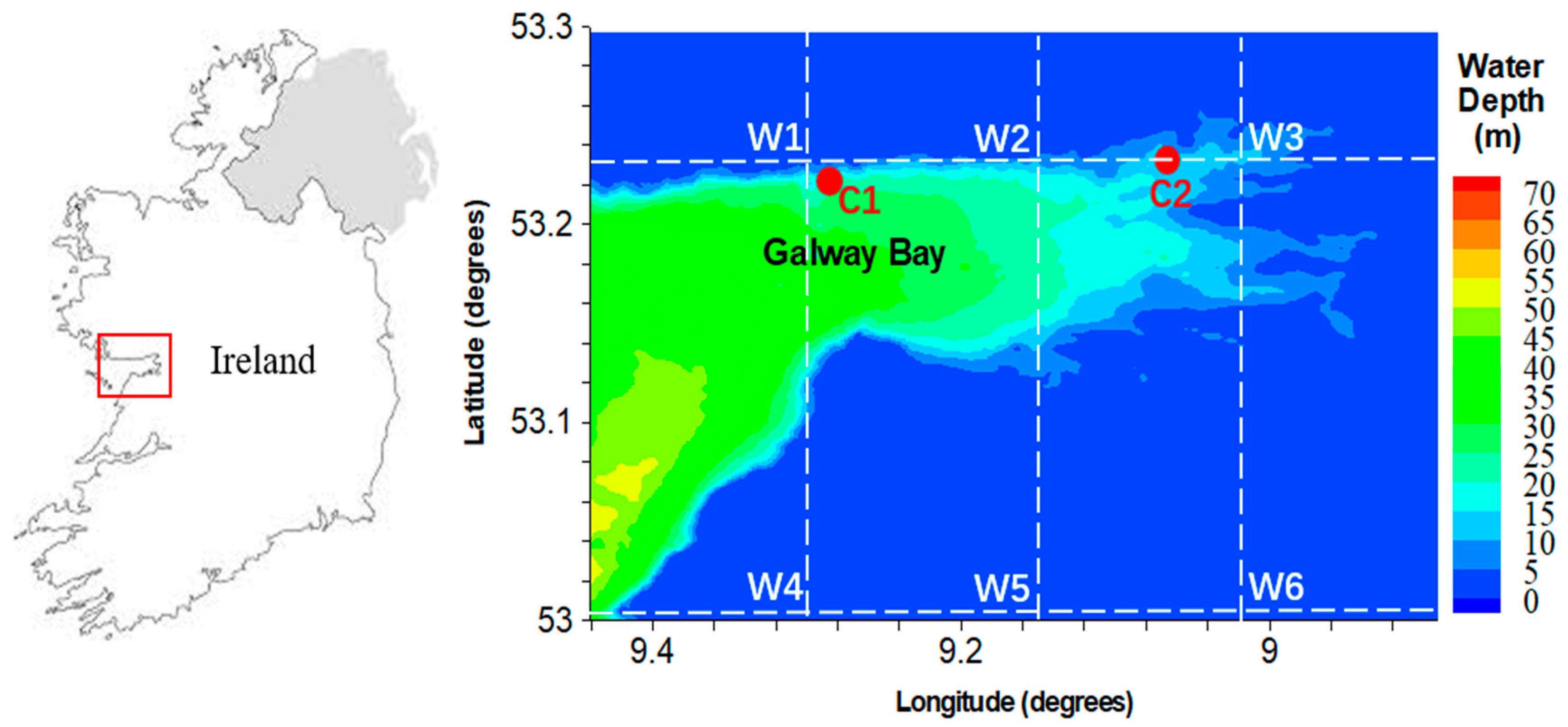
2.1. Research Domain
2.2. Observational Data
2.3. Numerical Model
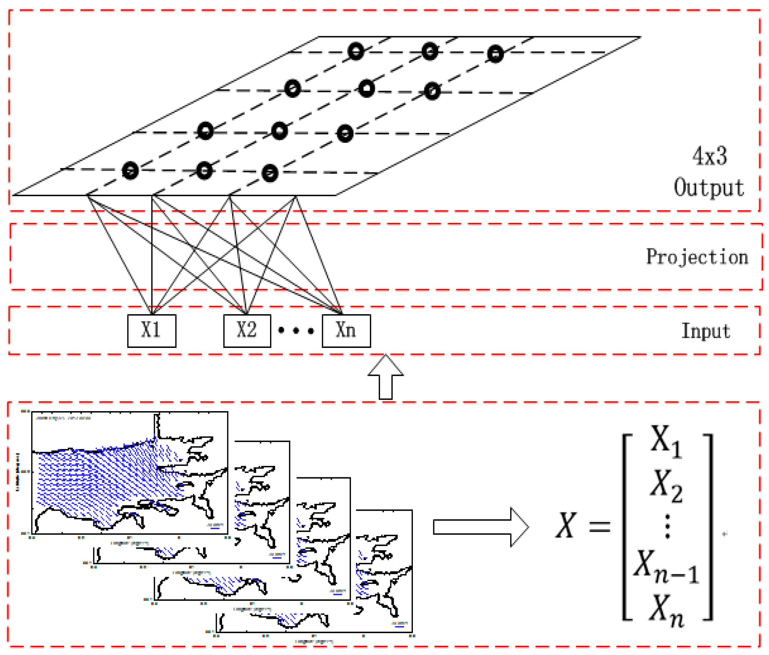
2.4. Self-Organizing Map
2.5. Empirical Orthogonal Function
3. Results
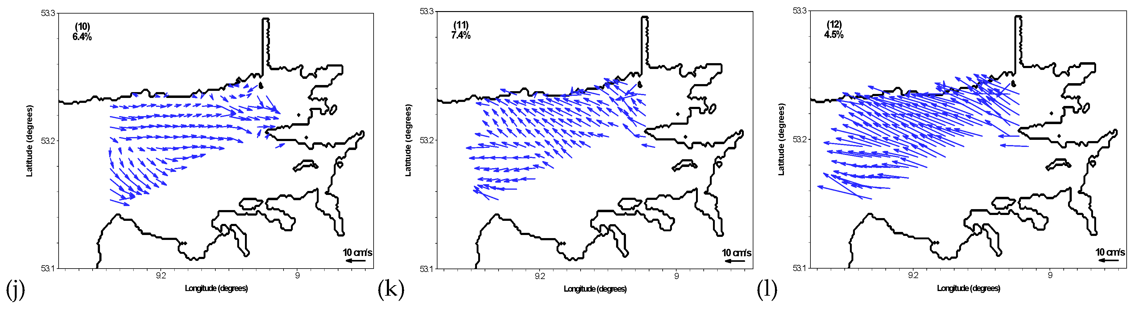
3.1. SOM Analysis
3.1.1. Spatial Variability
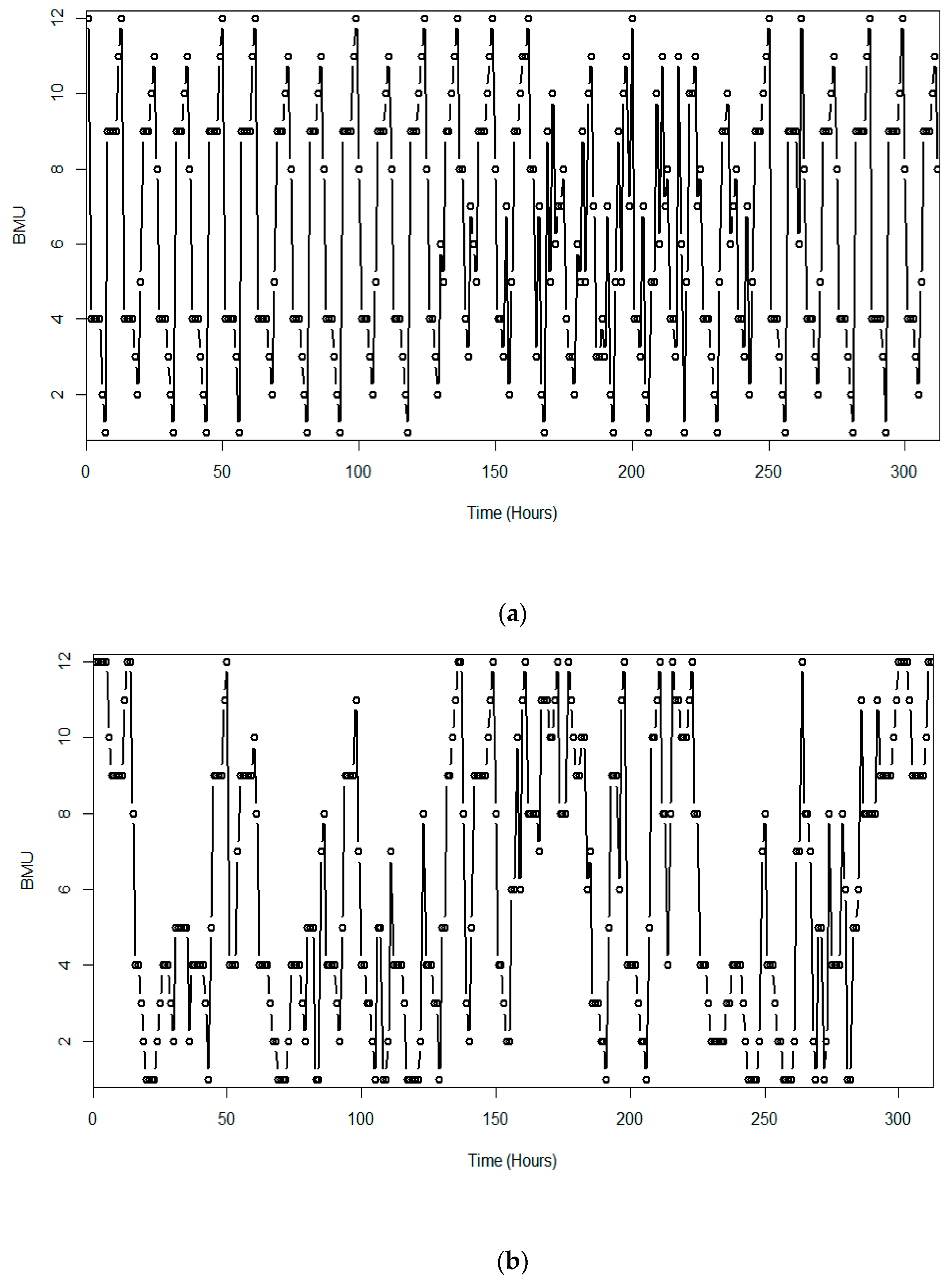
3.1.2. Temporal Evolution
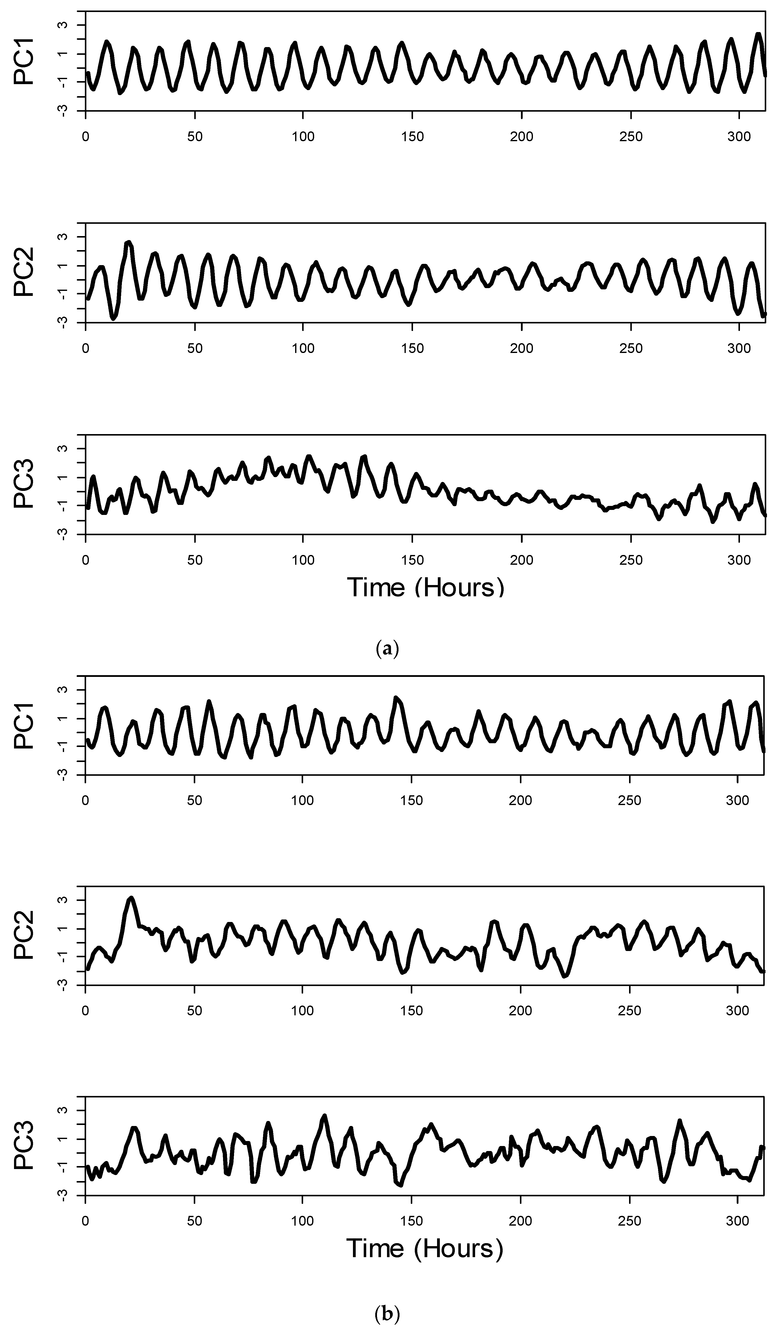
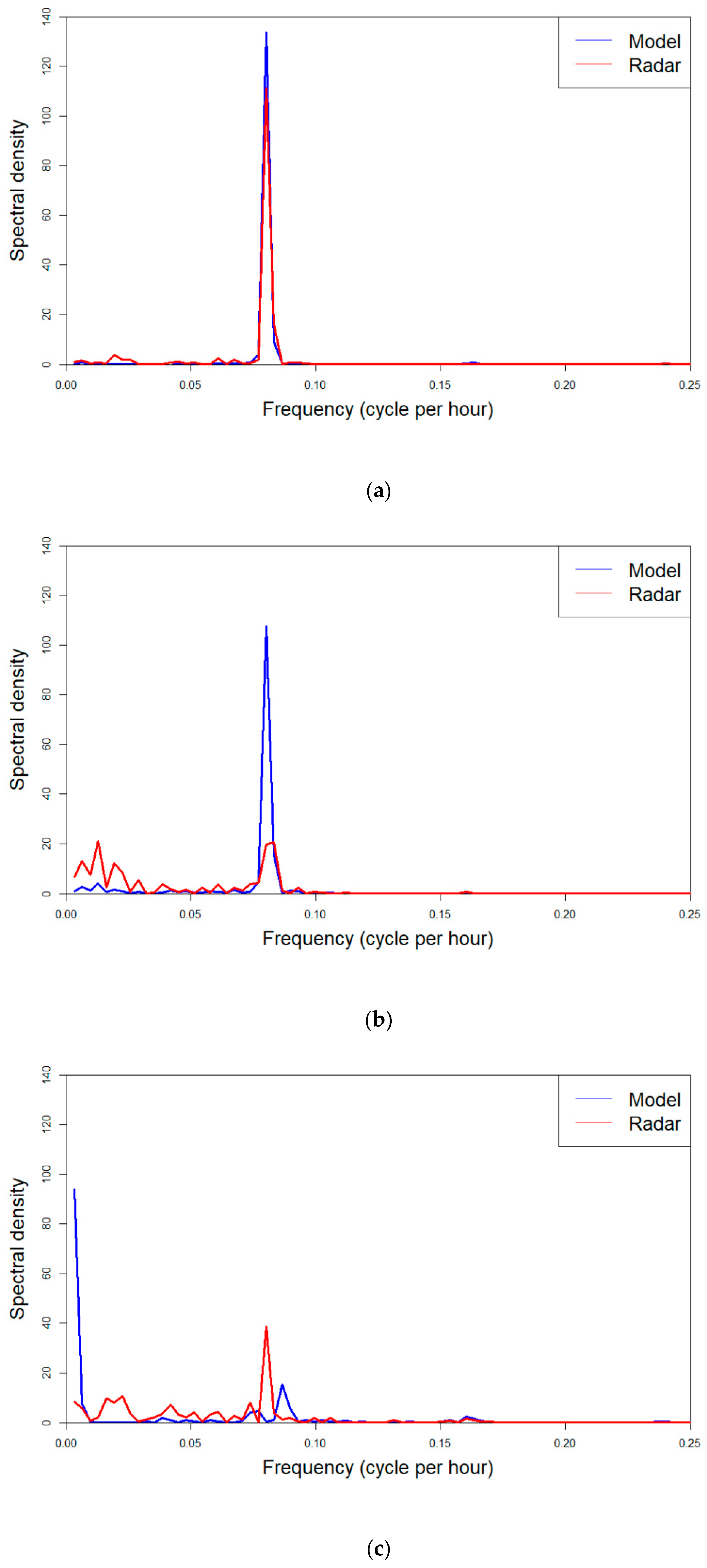
3.2. Empirical Orthogonal Function
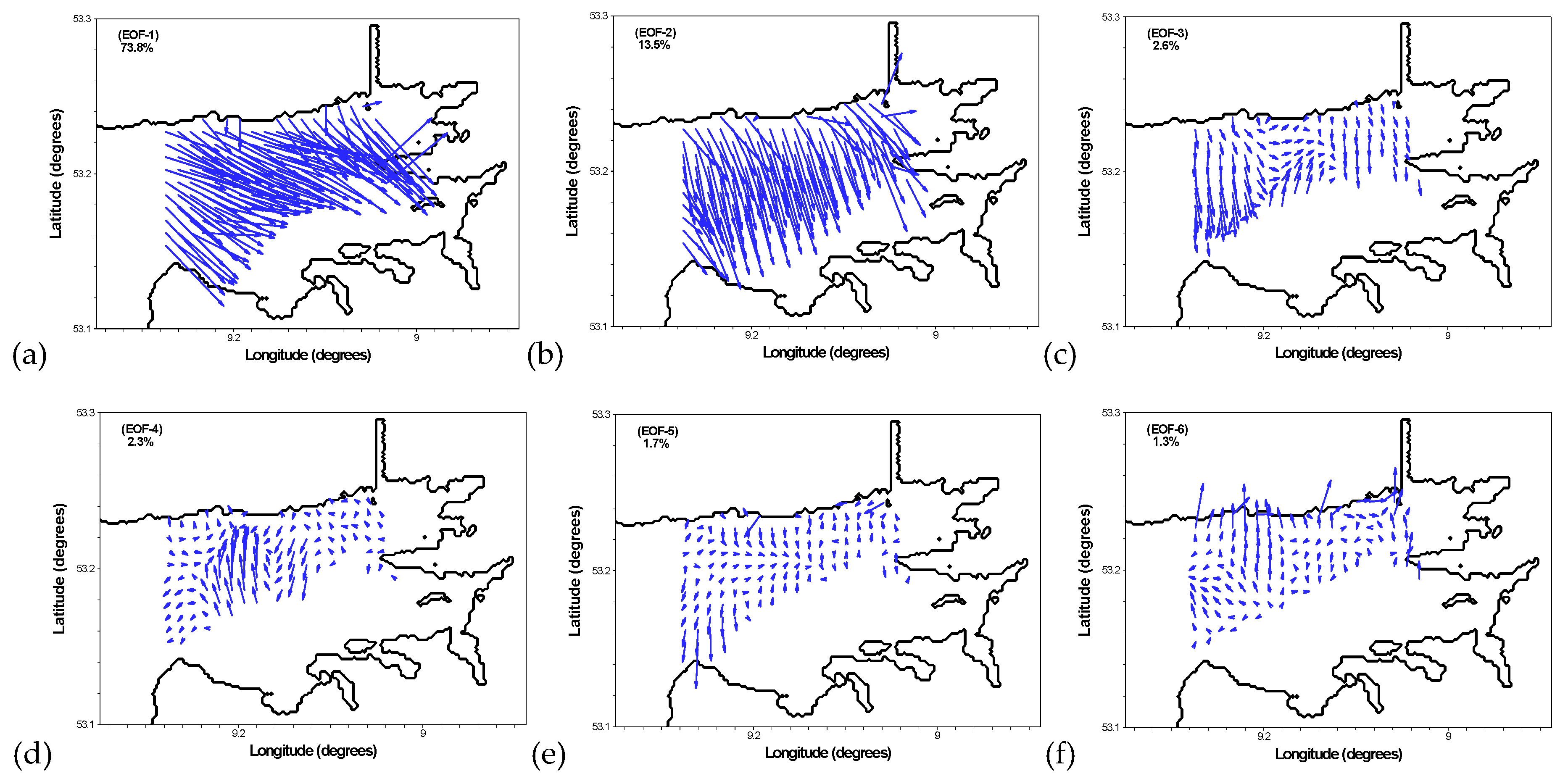
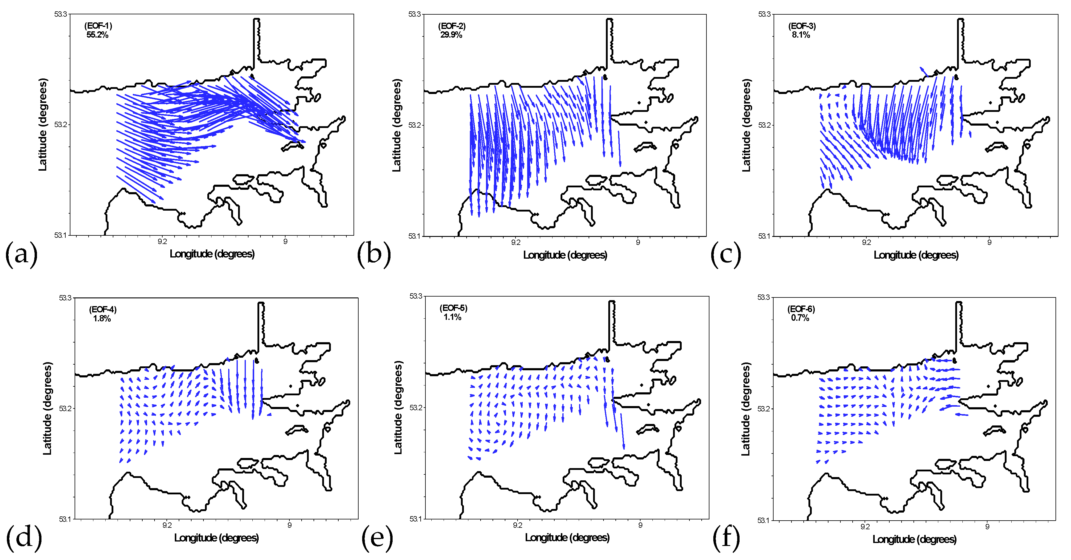
3.2.1. Spatial Modes
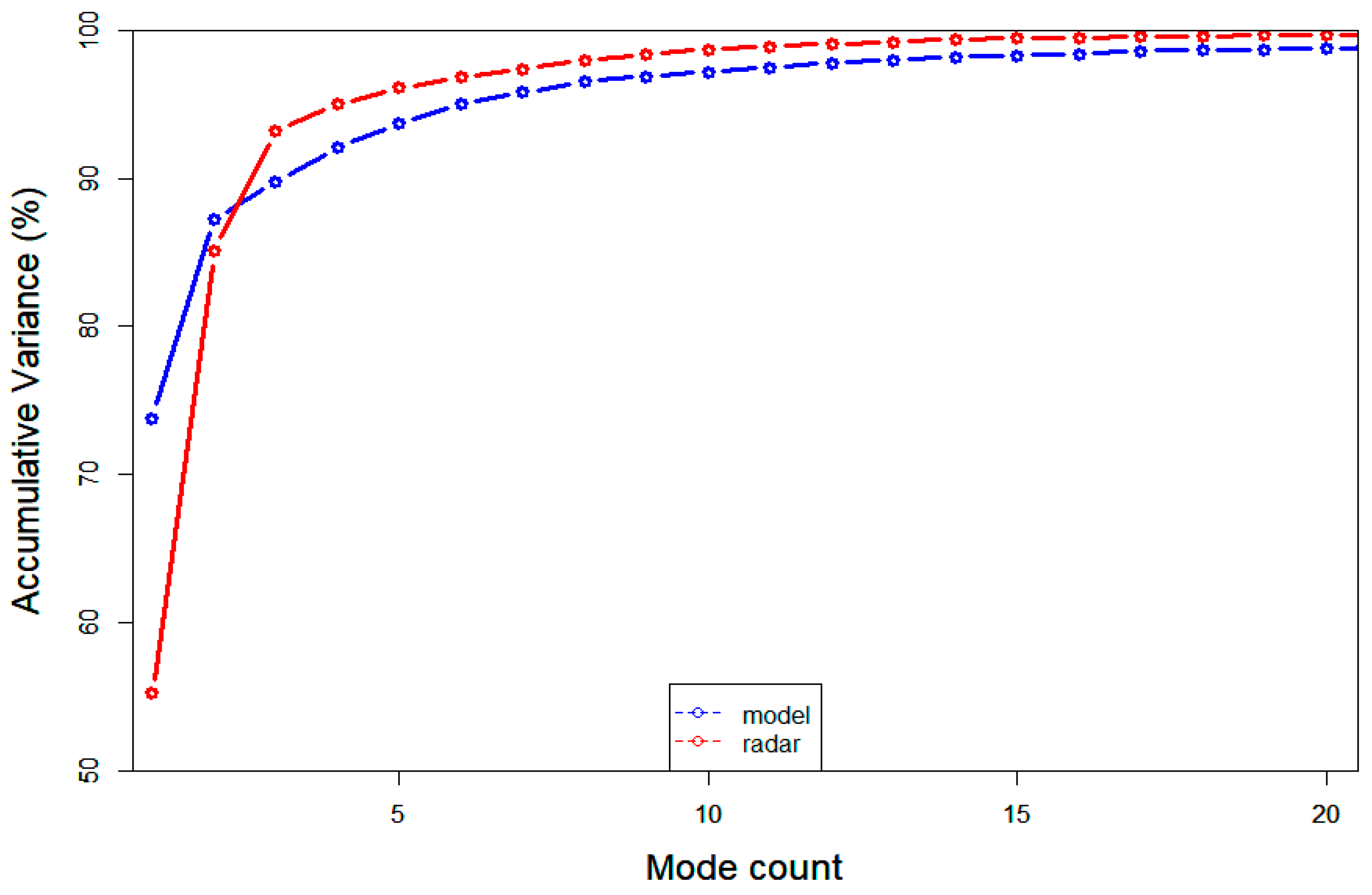
3.2.2. Variance of Surface Flows Explained by EOF Modes
4. Discussion
5. Conclusions
Author Contributions
Funding
Acknowledgments
Conflicts of Interest
Appendix A. Self-Organizing Map
- Determine the size and type of the map.
- Initialize each node’s weights at random.
- Select a vector at random from the training dataset and present to the network. The following Euclidean distance formula is calculated to assess the “best matching unit (BMU)” between each node and all input dataset.
Appendix B. Empirical Orthogonal Function
References
- Szuts, Z.B.; Bower, A.S.; Donohue, K.A.; Girton, J.B.; Hummon, J.M.; Katsumata, K.; Lumpkin, R.; Ortner, P.B.; Phillips, H.E.; Rossby, H.T.; et al. The Scientific and Societal Uses of Global Measurements of Subsurface Velocity. Front. Mar. Sci. 2019, 6, 6. [Google Scholar] [CrossRef]
- Farcy, P.; Durand, D.; Charria, G.; Painting, S.J.; Tamminem, T.; Collingridge, K.; Grémare, A.J.; Delauney, L.; Puillat, I. Toward a European Coastal Observing Network to Provide Better Answers to Science and to Societal Challenges; The JERICO Research Infrastructure. Front. Mar. Sci. 2019, 6. [Google Scholar] [CrossRef]
- Vandenbulcke, L.; Beckers, J.-M.; Barth, A. Correction of inertial oscillations by assimilation of HF radar data in a model of the Ligurian Sea. Ocean Dyn. 2016, 67, 117–135. [Google Scholar] [CrossRef]
- Lai, Y.; Zhou, H.; Yang, J.; Zeng, Y.; Wen, B. Submesoscale Eddies in the Taiwan Strait Observed by High-Frequency Radars: Detection Algorithms and Eddy Properties. J. Atmos. Ocean. Technol. 2017, 34, 939–953. [Google Scholar] [CrossRef]
- Hisaki, Y.; Kashima, M.; Kojima, S. Surface current patterns observed by HF radar: Methodology and analysis of currents to the north of the Yaeyama Islands, East China Sea. Ocean Dyn. 2016, 66, 329–352. [Google Scholar] [CrossRef]
- John, M.; Jena, B.K.; Sivakholundu, K.M. Surface current and wave measurement during cyclone phaillin by high frequency radars along the indian coast. Curr. Sci. 2015, 108, 405–409. [Google Scholar]
- Wang, Y.; Ma, X.; Joyce, M.J. Reducing sensor complexity for monitoring wind turbine performance using principal component analysis. Renew. Energy 2016, 97, 444–456. [Google Scholar] [CrossRef] [Green Version]
- Mardia, K.V. Some properties of classical multidimensional scaling. Commun. Stat. Theory Methods 1978, 7, 1233–1241. [Google Scholar] [CrossRef]
- Liu, Y.; Weisberg, R.H.; Vignudelli, S.; Mitchum, G.T. Patterns of the loop current system and regions of sea surface height variability in the eastern Gulf of Mexico revealed by the self-organizing maps. J. Geophys. Res. Oceans 2016, 121, 2347–2366. [Google Scholar] [CrossRef] [Green Version]
- Liu, Y.; Weisberg, R.H.; Shay, L.K. Current Patterns on the West Florida Shelf from Joint Self-Organizing Map Analyses of HF Radar and ADCP Data. J. Atmos. Ocean. Technol. 2007, 24, 702–712. [Google Scholar] [CrossRef]
- Soto-Navarro, J.; Lorente, P.; Fanjul, E.A.; Sanchez-Garrido, J.C.; Garcia-Lafuente, J. Surface circulation at the S trait of G ibraltar: A combined HF radar and high resolution model study. J. Geophys. Res. Oceans 2016, 121, 2016–2034. [Google Scholar] [CrossRef] [Green Version]
- Reusch, D.B.; Hewitson, B.C.; Alley, R.B. Towards ice-core-based synoptic reconstructions of west antarctic climate with artificial neural networks. Int. J. Clim. 2005, 25, 581–610. [Google Scholar] [CrossRef]
- Lobo, V.J.A.S. Application of Self Organizing Maps to the Maritime Environment. In Proceedings of the 4th International Workshop on Information Fusion and Geographical Information Systems, St Petersburg, Russia, 17–20 May 2009; Popovich, V.V., Schrenk, M., Claramunt, C., Korolenko, K.V., Eds.; Springer-Verlag Berlin: St Petersburg, Russia, 2009; pp. 19–36. [Google Scholar]
- Lin, G.-F.; Chen, L.-H. Identification of homogeneous regions for regional frequency analysis using the self-organizing map. J. Hydrol. 2006, 324, 1–9. [Google Scholar] [CrossRef]
- Solidoro, C.; Bandelj, V.; Barbieri, P.; Cossarini, G.; Umani, S.F. Understanding dynamic of biogeochemical properties in the northern Adriatic Sea by using self-organizing maps and k-means clustering. J. Geophys. Res. Space Phys. 2007, 112, 1–13. [Google Scholar] [CrossRef] [Green Version]
- Tsai, W.-P.; Huang, S.-P.; Cheng, S.-T.; Shao, K.-T.; Chang, F.-J. A data-mining framework for exploring the multi-relation between fish species and water quality through self-organizing map. Sci. Total. Environ. 2017, 579, 474–483. [Google Scholar] [CrossRef]
- Nkiaka, E.; Nawaz, N.R.; Lovett, J.C. Using self-organizing maps to infill missing data in hydro-meteorological time series from the Logone catchment, Lake Chad basin. Environ. Monit. Assess. 2016, 188, 1–12. [Google Scholar] [CrossRef] [Green Version]
- Tsui, I.-F.; Wu, C.-R. Variability analysis of Kuroshio intrusion through Luzon Strait using growing hierarchical self-organizing map. Ocean Dyn. 2012, 62, 1187–1194. [Google Scholar] [CrossRef]
- Camus, P.; Cofino, A.S.; Mendez, F.J.; Medina, R. Multivariate Wave Climate Using Self-Organizing Maps. J. Atmos. Ocean. Technol. 2011, 28, 1554–1568. [Google Scholar] [CrossRef]
- Kalteh, A.M.; Hjorth, P.; Berndtsson, R. Review of the self-organizing map (SOM) approach in water resources: Analysis, modelling and application. Environ. Model. Softw. 2008, 23, 835–845. [Google Scholar] [CrossRef]
- Liu, Y.; Weisberg, R.H.; He, R. Sea Surface Temperature Patterns on the West Florida Shelf Using Growing Hierarchical Self-Organizing Maps. J. Atmos. Ocean. Technol. 2006, 23, 325–338. [Google Scholar] [CrossRef] [Green Version]
- Reusch, D.B.; Alley, R.B.; Hewitson, B.C. North Atlantic climate variability from a self-organizing map perspective. J. Geophys. Res. Space Phys. 2007, 112, 1–20. [Google Scholar] [CrossRef]
- Liu, Y.; Weisberg, R.H. Patterns of ocean current variability on the West Florida Shelf using the self-organizing map. J. Geophys. Res. Space Phys. 2005, 110, 1–12. [Google Scholar] [CrossRef] [Green Version]
- Liu, Y.; Weisberg, R.H.; Mooers, C.N.K. Performance evaluation of the self-organizing map for feature extraction. J. Geophys. Res. Space Phys. 2006, 111, 111. [Google Scholar] [CrossRef]
- Mihanović, H.; Cosoli, S.; Vilibić, I.; Ivanković, D.; Dadić, V.; Gačić, M. Surface current patterns in the northern Adriatic extracted from high-frequency radar data using self-organizing map analysis. J. Geophys. Res. Space Phys. 2011, 116, 116. [Google Scholar] [CrossRef] [Green Version]
- Vilibić, I.; Šepić, J.; Mihanović, H.; Kalinic, H.; Cosoli, S.; Janeković, I.; Žagar, N.; Jesenko, B.; Tudor, M.; Dadić, V.; et al. Self-Organizing Maps-based ocean currents forecasting system. Sci. Rep. 2016, 6, 22924. [Google Scholar] [CrossRef]
- Jin, B.; Wang, G.; Liu, Y.; Zhang, R. Interaction between the East China Sea Kuroshio and the Ryukyu Current as revealed by the self-organizing map. J. Geophys. Res. Space Phys. 2010, 115, 1–7. [Google Scholar] [CrossRef] [Green Version]
- Barros, A.P.; Bowden, G.J. Toward long-lead operational forecasts of drought: An experimental study in the Murray-Darling River Basin. J. Hydrol. 2008, 357, 349–367. [Google Scholar] [CrossRef]
- Obach, M.; Wagner, R.; Werner, H.; Schmidt, H.-H. Modelling population dynamics of aquatic insects with artificial neural networks. Ecol. Model. 2001, 146, 207–217. [Google Scholar] [CrossRef]
- Malek, S.; Gunalan, R.; Kedija, S.Y.; Lau, C.F.; Mosleh, M.A.A.; Milow, P.; Lee, S.A.; Saw, A. Random forest and Self Organizing Maps application for analysis of pediatric fracture healing time of the lower limb. Neurocomputing 2018, 272, 55–62. [Google Scholar] [CrossRef]
- Booth, D. The Water Structure and Circulation of Killary Harbour and of Galway Bay. Ph.D. Thesis, National University of Ireland, Galway, Ireland, 1975. [Google Scholar]
- Fernandes, L. A Study of the Oceanography of Galway Bay, Mid-Western Coastal Waters (Galway Bay to Bralle Bay), Shannon Estuary and the Rive Shannon Plume. Ph.D. Thesis, National University of Ireland, Galway, Ireland, 1988. [Google Scholar]
- Wen, L. Three-Dimensional Hydrodynamic Modelling in Galway Bay. Ph.D. Thesis, University College Galway, Galway, Ireland, 1995. [Google Scholar]
- Joshi, S.; Duffy, G.P.; Brown, C. Mobility of maerl-siliciclastic mixtures: Impact of waves, currents and storm events. Estuar. Coast. Shelf Sci. 2017, 189, 173–188. [Google Scholar] [CrossRef]
- Paduan, J.D.; Washburn, L. High-Frequency Radar Observations of Ocean Surface Currents. Annu. Rev. Mar. Sci. 2013, 5, 115–136. [Google Scholar] [CrossRef] [PubMed] [Green Version]
- Lipa, B.J.; Barrick, D.E.; Isaacson, J.; Lilieboe, P.M. Codar wave measurements from a north sea semisubmer sible. IEEE J. Ocean. Eng. 1990, 15, 119–125. [Google Scholar] [CrossRef]
- Emery, B.M.; Washburn, L.; Harlan, J.A. Evaluating Radial Current Measurements from CODAR High-Frequency Radars with Moored Current Meters. J. Atmos. Ocean. Technol. 2004, 21, 1259–1271. [Google Scholar] [CrossRef]
- Liu, Y.; Weisberg, R.H.; Merz, C.R.; Lichtenwalner, S.; Kirkpatrick, G.J. HF Radar Performance in a Low-Energy Environment: CODAR SeaSonde Experience on the West Florida Shelf. J. Atmos. Ocean. Technol. 2010, 27, 1689–1710. [Google Scholar] [CrossRef]
- Roarty, H.; Cook, T.; Hazard, L.; George, D.; Harlan, J.; Cosoli, S.; Wyatt, L.; Fanjul, E.A.; Terrill, E.; Otero, M.; et al. The Global High Frequency Radar Network. Front. Mar. Sci. 2019, 6, 1–26. [Google Scholar] [CrossRef]
- Mantovani, C.; Corgnati, L.; Horstmann, J.; Rubio, A.; Reyes, E.; Quentin, C.; Cosoli, S.; Asensio, J.L.; Mader, J.; Griffa, A. Best Practices on High Frequency Radar Deployment and Operation for Ocean Current Measurement. Front. Mar. Sci. 2020, 7. [Google Scholar] [CrossRef] [Green Version]
- Tinis, S.W.; Hodgins, D.O.; Fingas, M. Assimilation of radar measured surface current fields into a numerical model for oil spill modelling. Spill Sci. Technol. Bull. 1996, 3, 247–251. [Google Scholar] [CrossRef]
- Bellomo, L.; Griffa, A.; Cosoli, S.; Falco, P.; Gerin, R.; Iermano, I.; Kalampokis, A.; Kokkini, Z.; Lana, A.; Magaldi, M.G.; et al. Toward an integrated HF radar network in the Mediterranean Sea to improve search and rescue and oil spill response: The TOSCA project experience. J. Oper. Oceanogr. 2015, 8, 1–13. [Google Scholar] [CrossRef]
- Ren, L.; Nash, S.; Hartnett, M. Forecasting of Surface Currents via Correcting Wind Stress with Assimilation of High-Frequency Radar Data in a Three-Dimensional Model. Adv. Meteorol. 2016, 2016, 1–12. [Google Scholar] [CrossRef] [Green Version]
- Marmain, J.; Molcard, A.; Forget, P.; Barth, A.; Ourmières, Y. Assimilation of HF radar surface currents to optimize forcing in the northwestern Mediterranean Sea. Nonlinear Process. Geophys. 2014, 21, 659–675. [Google Scholar] [CrossRef]
- Xu, J.; Huang, J.; Gao, S.; Cao, Y. Assimilation of high frequency radar data into a shelf sea circulation model. J. Ocean. Univ. China 2014, 13, 572–578. [Google Scholar] [CrossRef]
- Ren, L.; Nash, S.; Hartnett, M. Renewable energies offshore. In Chapter 24 Data Assimilation with High-Frequency (HF) Radar Surface Currents at a Marine Renewable Energy Test Site; Soares, C.G., Ed.; CRC Press: London, UK, 2015. [Google Scholar]
- Solabarrieta, L.; Frolov, S.; Cook, M.; Paduan, J.; Rubio, A.; González, M.; Mader, J.; Charria, G. Skill Assessment of HF Radar–Derived Products for Lagrangian Simulations in the Bay of Biscay. J. Atmos. Ocean. Technol. 2016, 33, 2585–2597. [Google Scholar] [CrossRef] [Green Version]
- Roarty, H.; Glenn, S.; Allen, A. Evaluation of Environmental Data for Search and Rescue. In Proceedings of the OCEANS 2016, Shanghai, China, 10–13 April 2016; IEEE: Piscataway, NJ, USA, 2016; pp. 1–3. [Google Scholar]
- Cosoli, S.; Grcic, B.; De Vos, S.; Hetzel, Y. Improving Data Quality for the Australian High Frequency Ocean Radar Network through Real-Time and Delayed-Mode Quality-Control Procedures. Remote. Sens. 2018, 10, 1476. [Google Scholar] [CrossRef] [Green Version]
- Kim, S.Y.; Terrill, E.; Cornuelle, B. Objectively mapping HF radar-derived surface current data using measured and idealized data covariance matrices. J. Geophys. Res. Space Phys. 2007, 112, 112. [Google Scholar] [CrossRef] [Green Version]
- O’Donncha, F.; Hartnett, M.; Nash, S.; Ren, L.; Ragnoli, E. Characterizing observed circulation patterns within a bay using HF radar and numerical model simulations. J. Mar. Syst. 2015, 142, 96–110. [Google Scholar] [CrossRef]
- Rubio, A.; Mader, J.; Corgnati, L.; Mantovani, C.; Griffa, A.; Novellino, A.; Quentin, C.; Wyatt, L.; Schulz-Stellenfleth, J.; Horstmann, J.; et al. HF Radar Activity in European Coastal Seas: Next Steps toward a Pan-European HF Radar Network. Front. Mar. Sci. 2017, 4. [Google Scholar] [CrossRef] [Green Version]
- Ren, L.; Nagle, D.; Hartnett, M.; Nash, S. The Effect of Wind Forcing on Modeling Coastal Circulation at a Marine Renewable Test Site. Energies 2017, 10, 2114. [Google Scholar] [CrossRef] [Green Version]
- Ren, L.; Nash, S.; Hartnett, M. Observation and modeling of tide-and wind-induced surface currents in Galway Bay. Water Sci. Eng. 2015, 8, 345–352. [Google Scholar] [CrossRef] [Green Version]
- Hamrick, J.M. Efdc Technical Memorandum; Tetra Tech: Fairfax, VA, USA, 2006. [Google Scholar]
- Tetra Tech, Inc. The Environmental Fluid Dynamics Code Theory and Computation Volume 1: Hydrodynamics and Mass Transport; Tetra Tech, Inc.: Fairfax, VA, USA, 2007; p. 60. [Google Scholar]
- Hamrick, J.M. A Three-Dimensional Environmental Fluid Dynamics Computer Code: Therotical and Computatonal Aspects; Virginia Institute of Marine Science, William & Mary: Gloucester Point, VA, USA, 1992. [Google Scholar]
- Zou, R.; Carter, S.; Shoemaker, L.; Parker, A.; Henry, T. Integrated Hydrodynamic and Water Quality Modeling System to Support Nutrient Total Maximum Daily Load Development for Wissahickon Creek, Pennsylvania. J. Environ. Eng. 2006, 132, 555–566. [Google Scholar] [CrossRef]
- Jin, K.-R.; Ji, Z.-G. Case Study: Modeling of Sediment Transport and Wind-Wave Impact in Lake Okeechobee. J. Hydraul. Eng. 2004, 130, 1055–1067. [Google Scholar] [CrossRef]
- O’Donncha, F.; Hartnett, M.; Nash, S. Physical and numerical investigation of the hydrodynamic implications of aquaculture farms. Aquac. Eng. 2013, 52, 14–26. [Google Scholar] [CrossRef]
- Bôas, A.B.V.; Ardhuin, F.; Ayet, A.; Bourassa, M.A.; Brandt, P.; Chapron, B.; Cornuelle, B.D.; Farrar, J.T.; Fewings, M.R.; Fox-Kemper, B.; et al. Integrated Observations of Global Surface Winds, Currents, and Waves: Requirements and Challenges for the Next Decade. Front. Mar. Sci. 2019, 6. [Google Scholar] [CrossRef]
- Egbert, G.D.; Erofeeva, S.Y. Effificient inverse modeling of barotropic ocean tides. J. Atmos. Ocean. Technol. 2002, 19, 183. [Google Scholar] [CrossRef] [Green Version]
- Padman, L.; Erofeeva, S. A barotropic inverse tidal model for the Arctic Ocean. Geophys. Res. Lett. 2004, 31, 1–4. [Google Scholar] [CrossRef]
- Kohonen, T. Self-organized formation of topologically correct feature maps. Boil. Cybern. 1982, 43, 59–69. [Google Scholar] [CrossRef]
- Chalasani, R.; Principe, J.C. Self-organizing maps with information theoretic learning. Neurocomputing 2015, 147, 3–14. [Google Scholar] [CrossRef] [Green Version]
- Vilibić, I.; Kalinic, H.; Mihanović, H.; Cosoli, S.; Tudor, M.; Žagar, N.; Jesenko, B. Sensitivity of HF radar-derived surface current self-organizing maps to various processing procedures and mesoscale wind forcing. Comput. Geosci. 2015, 20, 115–131. [Google Scholar] [CrossRef]
- Vilibić, I.; Mihanović, H.; Kušpilić, G.; Ivčević, A.; Milun, V. Mapping of oceanographic properties along a middle Adriatic transect using Self-Organising Maps. Estuar. Coast. Shelf Sci. 2015, 163, 84–92. [Google Scholar] [CrossRef]
- Li, Q.; Chen, P.; Sun, L.; Ma, X. A global weighted mean temperature model based on empirical orthogonal function analysis. Adv. Space Res. 2018, 61, 1398–1411. [Google Scholar] [CrossRef]
- Hannachi, A.; Jolliffe, I.T.; Stephenson, D.B. Empirical orthogonal functions and related techniques in atmospheric science: A review. Int. J. Clim. 2007, 27, 1119–1152. [Google Scholar] [CrossRef]
- Monahan, A.H.; Fyfe, J.C.; Ambaum, M.H.; Stephenson, D.B.; North, G.R. Empirical Orthogonal Functions: The Medium is the Message. J. Clim. 2009, 22, 6501–6514. [Google Scholar] [CrossRef] [Green Version]
- Mau, J.-C.; Wang, D.-P.; Ullman, D.S.; Codiga, D.L. Characterizing Long Island Sound outflows from HF radar using self-organizing maps. Estuar. Coast. Shelf Sci. 2007, 74, 155–165. [Google Scholar] [CrossRef]
- Taylor, R. Interpretation of the Correlation Coefficient: A Basic Review. J. Diagn. Med. Sonogr. 1990, 6, 35–39. [Google Scholar] [CrossRef]
- Paduan, J.D.; Shulman, I. HF radar data assimilation in the Monterey Bay area. J. Geophys. Res. Space Phys. 2004, 109, 434–446. [Google Scholar] [CrossRef]


| Group | SOM Pattern | Representative Characteristics | Total Occurrence Frequency (%) |
|---|---|---|---|
| 1 | 1/5/6/9/10 | southeastward and eastward flows | 41.1 |
| 2 | 3/4/7/8, | western flows | 40.4 |
| 3 | 11/12 | northwestward flows | 11.9 |
| 4 | 2 | southwestward and alongshore flows | 6.7 |
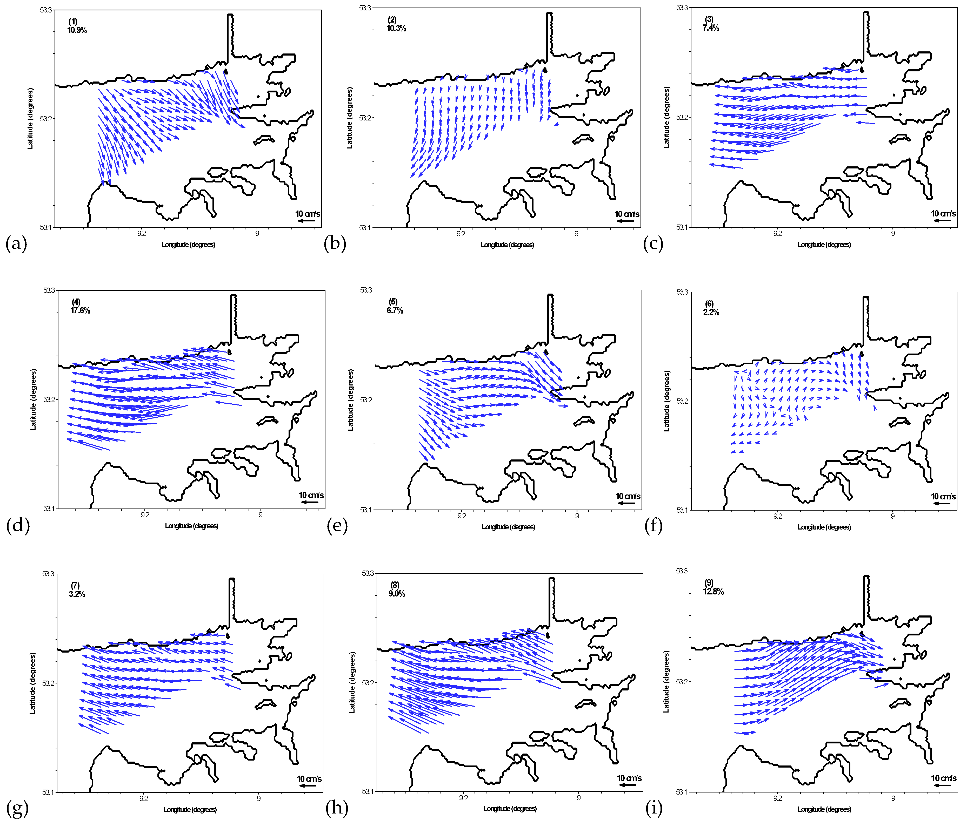
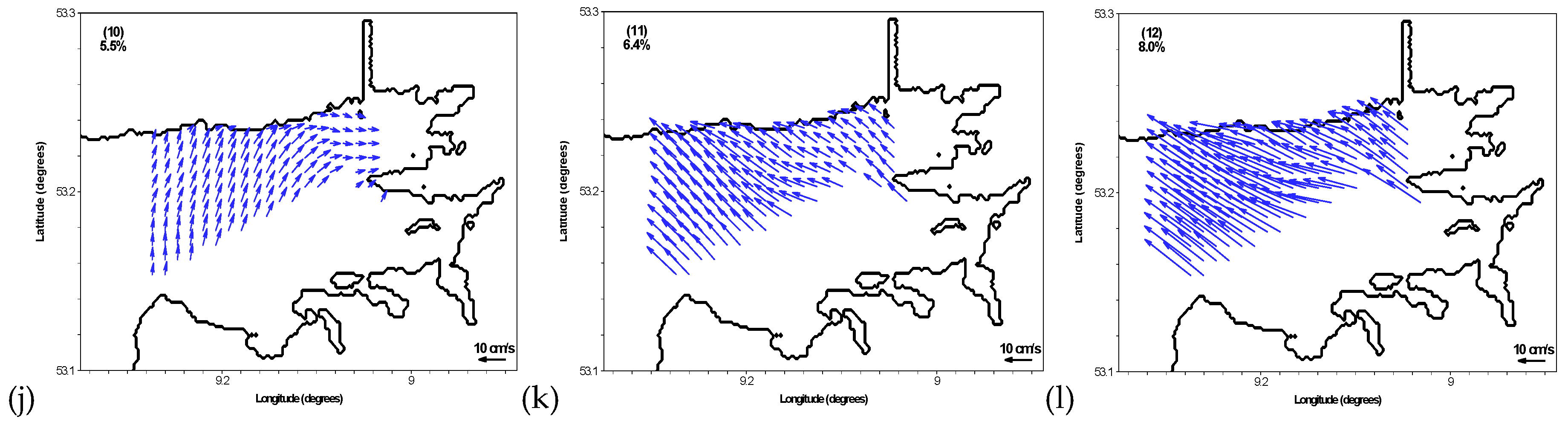
| Group | SOM Pattern | Representative Characteristics of Surface Vector Fields | Occurrence Frequency (%) |
|---|---|---|---|
| 1 | 3/4/7/8 | western flows | 37.2 |
| 2 | 1/5 | southeastward and alongshore flows | 17.6 |
| 3 | 9/10 | northeastward and alongshore flows | 18.3 |
| 4 | 2 | southern and southwestward flows | 10.3 |
| 5 | 6 | southwestward and northeastward flows | 2.2 |
| 6 | 11/12 | northwestward flows | 14.4 |
| EOF Mode | Variance (%) | Accumulative Variance (%) | ||
|---|---|---|---|---|
| EFDC | HFR | EFDC | HFR | |
| 1 | 73.8 | 55.2 | 73.8 | 55.2 |
| 2 | 13.5 | 29.9 | 87.2 | 85.1 |
| 3 | 2.6 | 8.1 | 89.9 | 93.2 |
| 4 | 2.3 | 1.8 | 92.1 | 95.0 |
| 5 | 1.7 | 1.1 | 93.7 | 96.1 |
| 6 | 1.3 | 0.7 | 95.0 | 96.8 |
© 2020 by the authors. Licensee MDPI, Basel, Switzerland. This article is an open access article distributed under the terms and conditions of the Creative Commons Attribution (CC BY) license (http://creativecommons.org/licenses/by/4.0/).
Share and Cite
Ren, L.; Chu, N.; Hu, Z.; Hartnett, M. Investigations into Synoptic Spatiotemporal Characteristics of Coastal Upper Ocean Circulation Using High Frequency Radar Data and Model Output. Remote Sens. 2020, 12, 2841. https://doi.org/10.3390/rs12172841
Ren L, Chu N, Hu Z, Hartnett M. Investigations into Synoptic Spatiotemporal Characteristics of Coastal Upper Ocean Circulation Using High Frequency Radar Data and Model Output. Remote Sensing. 2020; 12(17):2841. https://doi.org/10.3390/rs12172841
Chicago/Turabian StyleRen, Lei, Nanyang Chu, Zhan Hu, and Michael Hartnett. 2020. "Investigations into Synoptic Spatiotemporal Characteristics of Coastal Upper Ocean Circulation Using High Frequency Radar Data and Model Output" Remote Sensing 12, no. 17: 2841. https://doi.org/10.3390/rs12172841