Technical Note

Highly Local Model Calibration with a New GEDI LiDAR Asset on Google Earth Engine Reduces Landsat Forest Height Signal Saturation

1
US Forest Service Rocky Mountain Research Station, Ogden, UT 84401, USA
2
Google Inc., Google Switzerland, 8002 Zurich, Switzerland
3
Google Inc., Mountain View, CA 94043, USA
*
Author to whom correspondence should be addressed.
Remote Sens. 2020, 12(17), 2840; https://doi.org/10.3390/rs12172840
Submission received: 31 July 2020 / Revised: 26 August 2020 / Accepted: 31 August 2020 / Published: 1 September 2020
(This article belongs to the Special Issue Lidar Remote Sensing of Forest Structure, Biomass and Dynamics)

Abstract

:
While Landsat has proved to be effective for monitoring many elements of forest condition and change, the platform has well-documented limitations in measuring forest structure, the vertical distribution of the canopy. This is important because structure determines several key ecosystem functions, including: carbon storage; habitat suitability; and timber volume. Canopy structure is directly measured by LiDAR, and it should be possible to train Landsat structure models at a highly local scale with the dense, global sample of full waveform LiDAR observations collected by NASA’s Global Ecosystem Dynamics Investigation (GEDI). Local models are expected to perform better because: (a) such models may take advantage of localized correlations between structure and canopy surface reflectance; and (b) to the extent that models revert to the mean of the calibration data due to a lack of discrimination, local models will revert to a more representative mean. We tested Landsat-based relative height predictions using a new GEDI asset on Google Earth Engine, described here. Mean prediction error declined by 23% and important prediction biases at the extremes of the range of canopy height dropped as model calibration became more local, minimizing forest structure signal saturation commonly associated with Landsat and other passive optical sensors. Our results suggest that Landsat-based maps of structural variables such as height and biomass may substantially benefit from the kind of local calibration that GEDI’s dense sample of LiDAR data supports.

Graphical Abstract

1. Introduction

The spatial, temporal, and spectral resolution of data collected by the Landsat platform has proved appropriate for a range of important ecosystem monitoring applications [1,2]. However, Landsat has been used to study forest structure variables with only moderate success. As a passive optical sensor, Landsat’s reflectance signal is primarily determined by reflective properties of the top of the forest canopy; structural elements related to height are generally not directly sensed. The signal saturation that occurs when trees continue to grow below a closed canopy can limit differentiation of biomass levels [3,4,5] and other aspects of forest structure [4,6,7].
There is nevertheless ample motivation to develop strategies for using Landsat to map structure. No other space-based platform offers Landsat’s potential for historical perspective related to forest height and structure. Relying upon consistent radiometric processing since the mid-1980s [8], several studies have calibrated a forest structure-related model in one part of a time series and applied that model to imagery from different years [9,10,11]. Landsat can also contribute, when combined with a sample of high-quality reference data, to statistical estimates of population parameters such as mean biomass [12,13,14].
While Landsat may not respond to sub-canopy forest structure directly, structure is often at least somewhat correlated with Landsat reflectances, particularly in the shortwave infrared range. Landsat reflectances, or metrics derived from these, such as local texture, may in some cases be sensitive to canopy traits involving shading or moisture content, which are themselves correlated with structural variables [15,16]. Structure models are most likely to be accurate when restricted to local areas or specific forest types. Zhao et al. [17] found that stratifying Landsat-based biomass models by topographic aspect increased the amount of variation explained. Foody et al. [18] found that accurate Landsat-based biomass models could be trained at the site level, but that transfer of those models to other sites substantially reduced performance. They speculated that the contribution of local forest structure and composition to the remotely sensed response differed in important ways across sites. Locally trained models may minimize this cross-site uncertainty. Additionally, in extreme cases where a model has no basis for differentiation and simply predicts the mean of the training data, error will likely be lower if training and prediction occur over a narrower ecological range.
Spaceborne LiDAR datasets have the potential to provide canopy height measurements at densities sufficient to train a different height model every few kilometers. Several studies have used waveforms from the GLAS sensor on the ICESat platform to greatly expand the amount of training data available for height or biomass models using Landsat or MODIS as independent variables [19,20,21]. NASA’s Global Ecosystem Dynamics Investigation (GEDI) is a waveform LiDAR sensor mounted on the International Space Station, which overflies latitudes between 51.6° N & S. GEDI will provide significantly more waveform LiDAR observations than GLAS, using an acquisition strategy designed to maximize coverage of the world’s tropical and temperate forests [22].
The width of GEDI’s observation footprint, approximately 25 m [23], roughly corresponds to Landsat’s 30 m pixel size, allowing more straightforward footprint-to-pixel matching. We hypothesize that prediction error for canopy height, as a representative structure variable, will decline as Landsat-based models are fitted with GEDI measurements at increasingly local scales, such that longstanding signal saturation problems will be substantially diminished. Testing this hypothesis on a global scale requires a tool that allows flexible combination of the Landsat and GEDI data records. Accordingly, we introduce a raster-based GEDI asset on Google Earth Engine (GEE) [24], a cloud-based platform that provides both access to the entire Landsat archive (and other key datasets) and a powerful application programming interface. This publicly accessible GEDI asset, described below, will be maintained and updated throughout the mission.

2. Materials and Methods

2.1. GEDI Relative Height Data on Google Earth Engine

The GEDI GEE asset is constructed from a subset of the variables contained in the GEDI L2A Global Footprint-Level Elevation and Height Metrics Product [25], which is publicly available from the NASA Land Processes Distributed Active Archive Center (DAAC). This subset includes 12 identification and quality flag variables and 10 relative height (RH) values thought to be useful for forest structure modeling (Table 1). The reader is directed to the DAAC for definitions and processing details for each variable. For each mission month, all footprints having a quality value of 1 and having a “leaf-on” label according to the phenology map used by GEDI are rasterized in a 25-m resolution, 22-band image collection available through GEE. This image collection is not an official NASA product, but instead represents a reformatted version of publicly available GEDI data that is designed to work seamlessly with other spatial data on GEE.
For pixels containing more than one “quality” footprint in a given month, the rasterized image represents data from the footprint with the higher sensitivity value. Individual raster images were created over each UTM grid zone (6° longitude × 8° latitude; Figure 1). The most relevant variables for this paper are the fields showing relative height (rhNN, in meters), representing the height above the ground from below which a specified percentage of the laser’s energy returns (e.g., rh50 is the midpoint of the height distribution of returned energy). The GEDI GEE asset will be updated as new data are released and the entire archive is reprocessed. Documentation on GEE will note any changes to asset specifications.

2.2. Determining the Effect of Highly Local Forest Height Model Calibration Using GEDI Waveforms

A global sample of GEDI waveforms was drawn to test the performance of canopy height models calibrated at different scales. The sampled population of waveforms included data acquired from 25 March to 30 September 2019, which was all of the data publicly available at the time of this analysis. Only waveforms with a quality flag (see quality in Table 1) of 1 and falling in a forested cover class according to the CGLS LC100 land cover map from the Copernicus Global Land Survey [26] were considered here. The sample consisted of 10,000 forested waveforms, distributed randomly across UTM grid zones in numbers proportional to grid zone share of global forest cover according to the LC100 map (Figure 1).
At each waveform in the sample, 100 neighboring waveforms were randomly selected at 3 different scales: within 3 km, within 30 km, and on the same continent. Waveforms without at least 100 neighbors at the 3 km scale were excluded from the comparison, leaving 7615 of what are hereafter called “focal sites” (Figure 2). The rh98 value for each focal site was predicted with independent variables from Landsat (described below) three times, using a Random Forests model [27] calibrated with 100 randomly selected footprints at each of the three scales. Thus, three different models were built at each of 7615 focal sites: one with rh98 predicted from 100 neighboring GEDI shots within 3 km, one with 100 neighbors within 30 km, and one with 100 GEDI shots randomly selected from the same continent.
Predictions across the 7615 focal sites at each scale were compared to observed (and independent) focal site rh98 values. The effect of calibration scale was quantified by deriving both the root mean squared error (RMSE) and interquartile range of residual errors at each scale. Additionally, predictions were plotted in relation to observed values to assess systematic over- or under-prediction in regions along the range of rh98. Predictions were also evaluated by five global plant functional types, as mapped by Diaz et al. [28].
The Landsat predictor data were generated using harmonic functions [29] fitted to all cloud-free spectral values between 1999 and 2019 for pixels corresponding to each of the focal and neighbor sites. Specifically, these functions were fit with the ordinary least squares method and included terms that accommodate cyclical reflectance changes due to vegetation phenology. The function-fitting algorithm [29] features the same breakpoint generation function employed in the CCDC algorithm (Continuous Change Detection and Classification) [30]. Breaks generally indicate a land cover change [31], and the work reported here used only the harmonic function fit to imagery acquired since the date of the most recent breakpoint. Inputs to the Random Forest models included 60 independent variables: 8 parameters describing the harmonic fit for 6 reflectance bands (48 inputs); the RMSE of the fitted harmonic function for each band (6 inputs); and reflectance values for each of 6 Landsat bands predicted for 15 July 2019 by the harmonic functions. That date was arbitrary, but was near the mid-point of the GEDI data used in this analysis. No non-spectral variables were included in the models. Random Forest models used 500 decision trees, with one-third of the variables tried for each split.
It should be noted that rh98 does not equate to canopy top height. Differences between canopy height and rh98 may stem from: topography within the footprint, problems in correctly identifying ground elevation, and signal to noise uncertainty at the top of the canopy. The rh98 variable was selected here as a simple proxy for other forest structure variables.

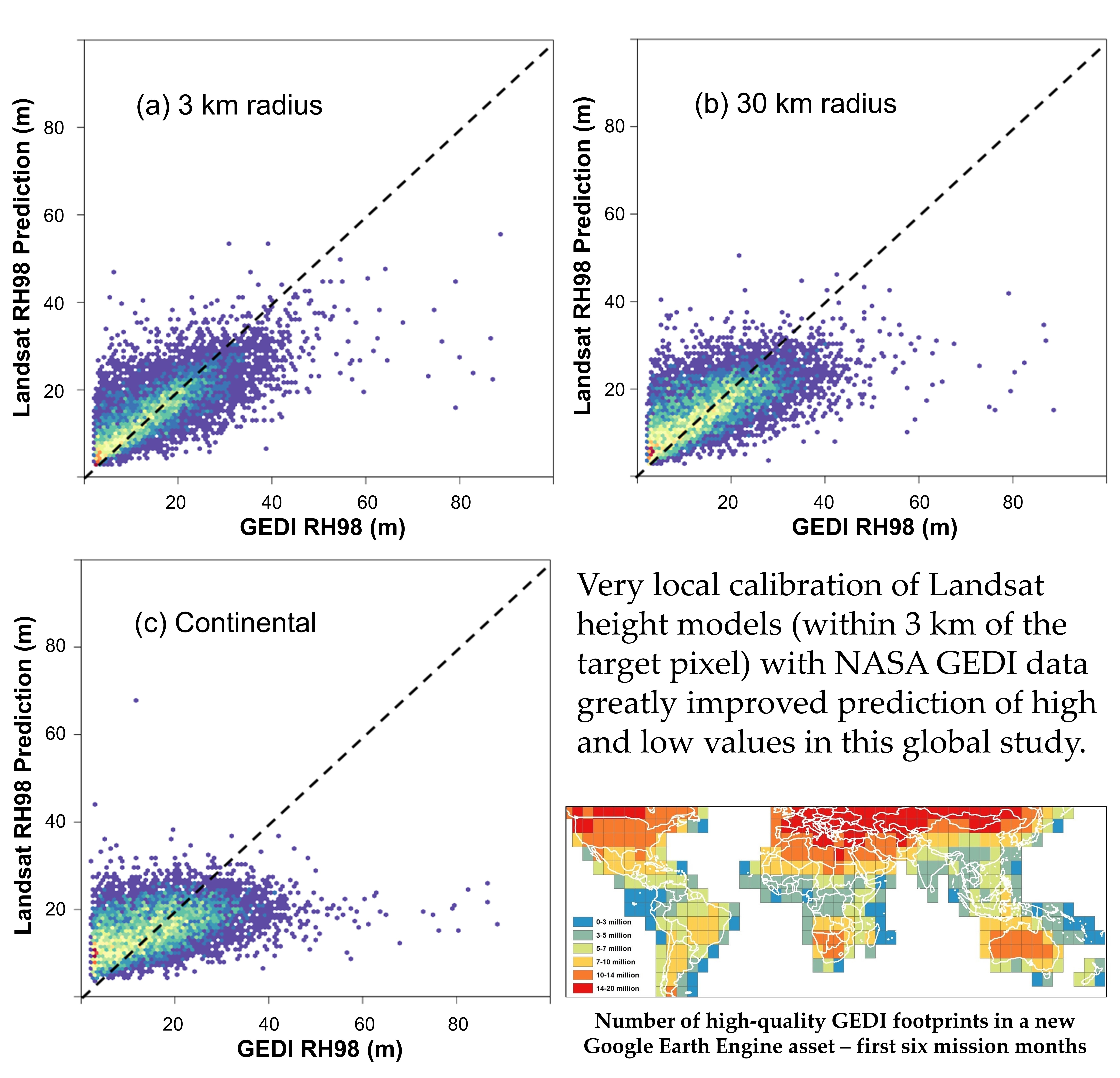
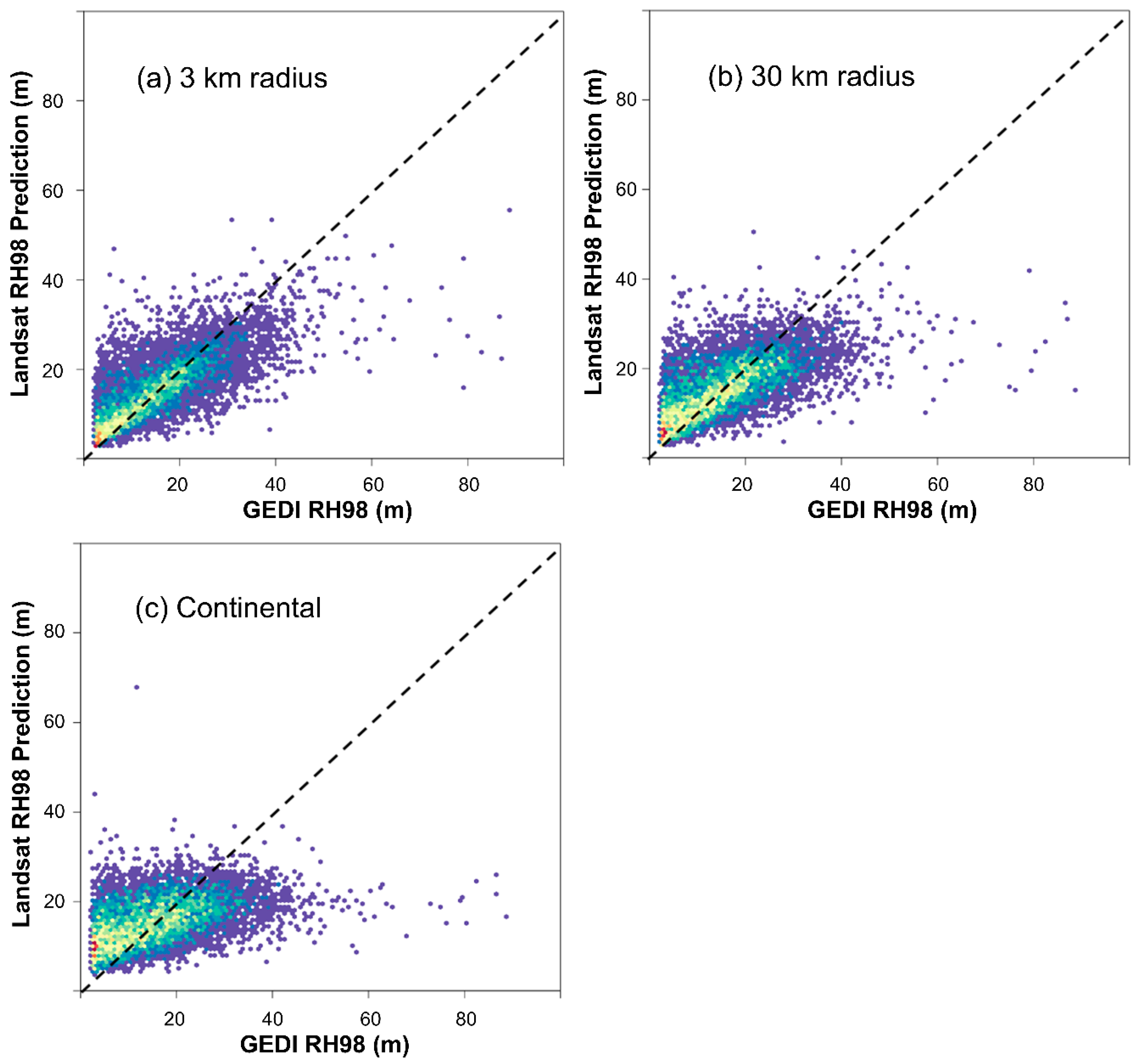
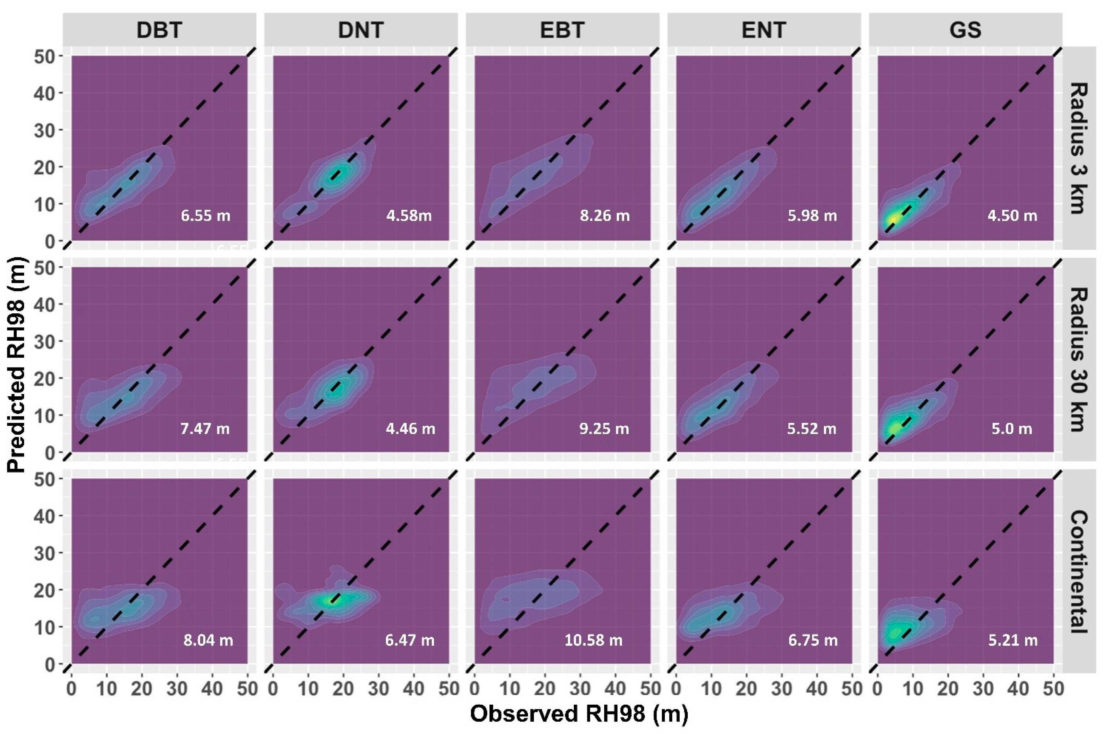
3. Results and Discussion

GEDI was designed to provide a sample, not a census, of the structure of the world’s temperate and tropical forests [22]. One of the mission’s primary science deliverables is a 1 × 1 km grid of biomass estimates (with estimated uncertainty), created with a hybrid model-based mode of inference that explicitly considers GEDI’s sampling design [32]. However, while GEDI’s spatially discontinuous design allows for clear, transparent estimation of biomass and other forest structure variables without the production of high-resolution maps, there are nevertheless important applications for such maps.
For instance, Tyukavina et al. [33] created a global canopy height map, similar to the maps created here, for the purpose of creating spatial strata to be used in the estimation of deforestation impacts on carbon emissions. Jantz et al. [34] used carbon maps to identify corridors between protected areas. Hansen et al. [35] overlaid a map of structurally complex forests with a map of lower human pressure to identify forests of high conservation value. Good Landsat-based maps will also be needed by the GEDI mission itself. In 1 km grid cells where the number of clear footprints is insufficient for making a sample-based estimate, a process called Hierarchical Model-Based inference will be used as a contingency. This approach uses biomass predictions at nearby GEDI footprints to train a second level of models to predict biomass using a wall-to-wall dataset such as Landsat [13]. The second-level model could be trained with the kind of 3 km search radius used here, for example, and applied to Landsat data to create GEDI biomass estimates for 1 km cells where sample-based estimates are not possible.
The results of the experiment reported here suggest that GEDI’s dense sample will partially mitigate well-known limitations due to Landsat forest structure signal saturation. The interquartile range of residual errors and the RMSE of predictions produced for the 7615 target cells declined as a function of decreasing size of the calibration window (Table 2). The impact of more local model calibration was even more evident when considering bias alone. When models lack a basis for discriminating different levels of the dependent variable, minimization of error (through whatever function the model employs) usually dictates predictions near the mean of the training data. The resulting overprediction of the low end of forest structure metrics and the underprediction of the high end have been noted elsewhere with the use of Landsat [36]. This phenomenon can result in maps that do not show the extreme conditions of a forest population. Furthermore, it can violate assumptions of homoskedasticity made in the formal modes of inference mentioned above. This pattern, clearly visible when Landsat models were calibrated at a continental scale, was diminished in models calibrated at 30 km and especially with models calibrated at 3 km (Figure 3).
Prediction uncertainty (Table 2) was high relative to other space-based LiDAR-based height models (e.g., [21]). There are several possible reasons for this. Our objective was to assess the effect of local calibration on models of canopy height based on Landsat. Other independent variables such as forest type and topography may have improved model performance but were excluded as peripheral to this objective. Additionally, the sample used here was subject to less screening than the samples used in many other papers. For example, we omitted shots determined through GEDI’s processing system to be contaminated by clouds, but we did not filter out shots on steep slopes, which is a step common to most published work with GLAS. Sensitivity of canopy height RMSE to even valid outliers was demonstrated by Simard et al. [37], who documented height RMSE going from 6.1 to 4.4 m with the exclusion of seven outliers. Our inclusion of sample locations in high-relief areas likely led to higher levels of assessed error, but it also led to an error metric more representative of global performance than one might produce with a more filtered dataset.
Improvements in high-low bias were not equal across the sample. Predictions of rh98 in evergreen needleleaf forests (ENT; 16% of all focal footprints) were closer to unity (predicted = observed) than other forest types when using continental calibration data (Figure 4). Better continental-scale calibration in this forest type may be related to the simpler or perhaps more uniform canopy form of coniferous trees. Coniferous forests have been observed to exhibit better relationships between Landsat and biomass than deciduous forests [17]. The biggest improvement occurred in evergreen broadleaf tree ecosystem (EBT), which are represented by half of the focal site sample. Figure 4 demonstrates little relationship between rh98 and the Landsat predictors for EBT when considered at the continental scale, with predictions occurring in an undifferentiated band across the entire range of observed rh98. Predictions of rh98 using a calibration range of 3 km, while not as tightly correlated with observed values as in other vegetation types, nevertheless represented a substantial gain in prediction accuracy, especially important because of the large extent of EBT.
The effectiveness of highly local calibration is likely due to some combination of: (1) restricting the range of ecological variability, thus simplifying the prediction task; and (2) ensuring that when models revert to prediction of the mean of the training data they at least revert to a more locally representative mean. This experiment randomly drew 100 neighbors to create separate pixel-level rh98 models at each scale of calibration. This ensured comparability across scales, but would not be operationally efficient for creating a global map. Extension to mapping applications would likely involve using a local tiling system, where all constituent clear footprints were used to train a tile-level model. The results presented here suggest that tiling should be as local as possible. Operational mapping may also include imagery from other sensors or stationary predictors related to topography or ownership class. Texture metrics applied to the Landsat-like Copernicus Sentinel-2 platform have also proven effective in training multispectral imagery from LiDAR returns [38].
It is noteworthy that only 7615 out of 10,000 sample locations had at least 100 neighbors within a 3 km range. Locations with insufficient neighbors might have occurred in isolated forest patches, such as on islands or in linear riparian areas, or they may simply have not been well sampled by the GEDI data collected prior to October, 2019 (representing approximately 25% of the measurements in GEDI’s original 2-year period of operation). Coverage should increase in both cases as the mission continues, and the results here suggest that finer scale calibration supported by additional LiDAR measurements will result in important reductions in Landsat forest structure signal saturation.

4. Conclusions

Highly local calibration of Landsat-based models of canopy height reduced both overall error and the tendency to over-predict the high end of the range and under-predict the low end. This suggests that spaceborne LiDAR data has potential to reduce long-acknowledged structure-mapping limitations of passive optical imagery. Combination of GEDI and Landsat data was facilitated by a new GEE GEDI asset that is announced and described in this Technical Note. Similar uses of GEDI waveform data with other wall-to-wall data sources optimized to be responsive to forest structure—new and upcoming radar instruments, for example—should likewise be possible and fruitful using cloud-based archives. As more GEDI data are collected, it will become possible to use smaller local neighborhoods, which has the potential to further improve maps of forest height and biomass across the globe.

Author Contributions

Conceptualization, S.P.H. and Z.Y.; methodology, S.P.H. and Z.Y.; software, Z.Y., N.G.; validation, Z.Y.; formal analysis, S.P.H. and Z.Y.; resources, N.G. and S.I.; data curation, S.I.; writing—original draft preparation, S.P.H.; writing—review and editing, S.P.H.; visualization, Z.Y.; supervision, S.P.H.; project administration, S.P.H.; funding acquisition, S.P.H., N.G. All authors have read and agreed to the published version of the manuscript.

Funding

This work was funded by NASA GEDI Interagency Agreement #RPO201523 (Healey) as part of NASA contract #NNL 15AA03C to the University of Maryland for the development and execution of the GEDI mission (Dubayah, Principal Investigator). Further funding was provided by NASA Carbon Monitoring System Grant #80HQTR18T0016 (Healey). The authors also appreciate support from the US Forest Service Rocky Mountain Research Station.

Acknowledgments

This work was possible because of the efforts of the GEDI Science Team. The authors are also grateful for technical support from Google and for insightful review comments from Ralph Dubayah.

Conflicts of Interest

The authors declare no conflict of interest.

References

  1. Cohen, W.B.; Goward, S. Landsat’s Role in Ecological Applications of Remote Sensing. Bioscience 2004, 54, 535–545. [Google Scholar] [CrossRef]
  2. Kennedy, R.E.; Yang, Z.; Cohen, W.B. Detecting trends in forest disturbance and recovery using yearly Landsat time series: 1. LandTrendr—Temporal segmentation algorithms. Remote Sens. Environ. 2010, 114, 2897–2910. [Google Scholar] [CrossRef]
  3. Lu, D.; Chen, Q.; Wang, G.; Moran, E.; Batistella, M.; Zhang, M.; Vaglio Laurin, G.; Saah, D. Aboveground Forest Biomass Estimation with Landsat and LiDAR Data and Uncertainty Analysis of the Estimates. Int. J. For. Res. 2012, 2012. [Google Scholar] [CrossRef]
  4. Carreiras, J.M.B.; Jones, J.; Lucas, R.M.; Shimabukuro, Y.E. Mapping major land cover types and retrieving the age of secondary forests in the Brazilian Amazon by combining single-date optical and radar remote sensing data. Remote Sens. Environ. 2017, 194, 16–32. [Google Scholar] [CrossRef] [Green Version]
  5. Avitabile, V.; Baccini, A.; Friedl, M.A.; Schmullius, C. Capabilities and limitations of Landsat and land cover data for aboveground woody biomass estimation of Uganda. Remote Sens. Environ. 2012, 117, 366–380. [Google Scholar] [CrossRef]
  6. Freitas, S.R.; Mello, M.C.S.; Cruz, C.B.M. Relationships between forest structure and vegetation indices in Atlantic Rainforest. For. Ecol. Manag. 2005, 218, 353–362. [Google Scholar] [CrossRef]
  7. Bawa, K.; Rose, J.; Ganeshaiah, K.N.; Barve, N.; Kiran, M.C.; Umashaanker, R. Assessing biodiversity from space: An example from the Western Ghats, India. Ecol. Soc. 2002, 6, 7. [Google Scholar] [CrossRef]
  8. Chander, G.; Markham, B.L.; Helder, D.L. Summary of current radiometric calibration coefficients for Landsat MSS, TM, ETM+, and EO-1 ALI sensors. Remote Sens. Environ. 2009, 113, 893–903. [Google Scholar] [CrossRef]
  9. Powell, S.L.; Cohen, W.B.; Healey, S.P.; Kennedy, R.E.; Moisen, G.G.; Pierce, K.B.; Ohmann, J.L. Quantification of live aboveground forest biomass dynamics with Landsat time-series and field inventory data: A comparison of empirical modeling approaches. Remote Sens. Environ. 2010, 114, 1053–1068. [Google Scholar] [CrossRef]
  10. Song, X.P.; Sexton, J.O.; Huang, C.; Channan, S.; Townshend, J.R. Characterizing the magnitude, timing and duration of urban growth from time series of Landsat-based estimates of impervious cover. Remote Sens. Environ. 2016, 175, 1–13. [Google Scholar] [CrossRef]
  11. Healey, S.P.; Yang, Z.; Cohen, W.B.; Pierce, D.J. Application of two regression-based methods to estimate the effects of partial harvest on forest structure using Landsat data. Remote Sens. Environ. 2006, 101, 115–126. [Google Scholar] [CrossRef]
  12. McRoberts, R.E. A model-based approach to estimating forest area. Remote Sens. Environ. 2006, 103, 56–66. [Google Scholar] [CrossRef]
  13. Saarela, S.; Holm, S.; Healey, S.P.; Andersen, H.E.; Petersson, H.; Prentius, W.; Patterson, P.L.; Næsset, E.; Gregoire, T.G.; Ståhl, G. Generalized hierarchical model-based estimation for aboveground biomass assessment using GEDI and landsat data. Remote Sens. 2018, 10, 1832. [Google Scholar] [CrossRef] [Green Version]
  14. Ståhl, G.; Saarela, S.; Schnell, S.; Holm, S.; Breidenbach, J.; Healey, S.P.; Patterson, P.L.; Magnussen, S.; Næsset, E.; McRoberts, R.E.; et al. Use of models in large-area forest surveys: Comparing model-assisted, model-based and hybrid estimation. For. Ecosyst. 2016, 3. [Google Scholar] [CrossRef] [Green Version]
  15. Cohen, W.B.; Spies, T.A.; Fiorella, M. Estimating the age and structure of forests in a multi-ownership landscape of western oregon, U.S.A. Int. J. Remote Sens. 1995, 16, 721–746. [Google Scholar] [CrossRef]
  16. Steininger, M.K. Satellite estimation of tropical secondary forest above-ground biomass: Data from Brazil and Bolivi. Int. J. Remote Sens. 2000, 21, 1139–1157. [Google Scholar] [CrossRef]
  17. Zhao, P.; Lu, D.; Wang, G.; Wu, C.; Huang, Y.; Yu, S. Examining spectral reflectance saturation in landsat imagery and corresponding solutions to improve forest aboveground biomass estimation. Remote Sens. 2016, 8, 469. [Google Scholar] [CrossRef] [Green Version]
  18. Foody, G.M.; Boyd, D.S.; Cutler, M.E.J. Predictive relations of tropical forest biomass from Landsat TM data and their transferability between regions. Remote Sens. Environ. 2003, 85, 463–474. [Google Scholar] [CrossRef]
  19. Chi, H.; Sun, G.; Huang, J.; Li, R.; Ren, X.; Ni, W.; Fu, A. Estimation of forest aboveground biomass in Changbai Mountain region using ICESat/GLAS and Landsat/TM data. Remote Sens. 2017, 9, 707. [Google Scholar] [CrossRef] [Green Version]
  20. Baccini, A.; Goetz, S.J.; Walker, W.S.; Laporte, N.T.; Sun, M.; Sulla-Menashe, D.; Hackler, J.; Beck, P.S.A.; Dubayah, R.; Friedl, M.A.; et al. Estimated carbon dioxide emissions from tropical deforestation improved by carbon-density maps. Nat. Clim. Chang. 2012, 358, 230–234. [Google Scholar] [CrossRef]
  21. Potapov, P.; Tyukavina, A.; Turubanova, S.; Talero, Y.; Hernandez-Serna, A.; Hansen, M.C.; Saah, D.; Tenneson, K.; Poortinga, A.; Aekakkararungroj, A.; et al. Annual continuous fields of woody vegetation structure in the Lower Mekong region from 2000–2017 Landsat time-series. Remote Sens. Environ. 2019, 232, 111278. [Google Scholar] [CrossRef]
  22. Dubayah, R.; Blair, J.B.; Goetz, S.; Fatoyinbo, L.; Hansen, M.; Healey, S.; Hofton, M.; Hurtt, G.; Kellner, J.; Luthcke, S.; et al. The Global Ecosystem Dynamics Investigation: High-Resolution laser ranging of the Earth’s forests and topography. Sci. Remote Sens. 2020, 1, 100002. [Google Scholar] [CrossRef]
  23. Hancock, S.; Armston, J.; Hofton, M.; Sun, X.; Tang, H.; Duncanson, L.I.; Kellner, J.R.; Dubayah, R. The GEDI Simulator: A Large-Footprint Waveform Lidar Simulator for Calibration and Validation of Spaceborne Missions. Earth Space Sci. 2019, 6, 294–310. [Google Scholar] [CrossRef] [PubMed]
  24. Gorelick, N.; Hancher, M.; Dixon, M.; Ilyushchenko, S.; Thau, D.; Moore, R. Google Earth Engine: Planetary-scale geospatial analysis for everyone. Remote Sens. Environ. 2017, 202, 18–27. [Google Scholar] [CrossRef]
  25. Dubayah, R.; Hofton, M.; Blair, J.B.; Armston, J.; Tang, H.; Luthcke, S. GEDI L2A Elevation and Height Metrics Data Global Footprint Level V001. NASA EOSDIS Land Processes DAAC. 2020. Available online: https://doi.org/10.5067/GEDI/GEDI02_A.001 (accessed on 31 August 2020).
  26. Buchhorn, M.; Smets, B.; Bertels, L.; Lesiv, M.; Tsendbazar, N.-E.; Herold, M.; Fritz, S. Copernicus Global Land Service: Land Cover 100m: Epoch 2015: Globe (Version V2.0.2) [Data set] 2019. Remote Sens. 2020, 12, 1044. [Google Scholar] [CrossRef] [Green Version]
  27. Breiman, L. Random forests. Mach. Learn. 2001, 45, 5–32. [Google Scholar] [CrossRef] [Green Version]
  28. Diaz, S.; Cabido, M. Plant functional types and ecosystem function in relation to global change. J. Veg. Sci. 1997, 8, 463–474. [Google Scholar] [CrossRef]
  29. Zhu, Z.; Zhang, J.; Yang, Z.; Aljaddani, A.H.; Cohen, W.B.; Qiu, S.; Zhou, C. Continuous monitoring of land disturbance based on Landsat time series. Remote Sens. Environ. 2020, 238. [Google Scholar] [CrossRef]
  30. Zhu, Z.; Woodcock, C.E. Continuous change detection and classification of land cover using all available Landsat data. Remote Sens. Environ. 2014, 144, 152–171. [Google Scholar] [CrossRef] [Green Version]
  31. Cohen, W.B.; Healey, S.P.; Yang, Z.; Stehman, S.V.; Brewer, C.K.; Brooks, E.B.; Gorelick, N.; Huang, C.; Hughes, M.J.; Kennedy, R.E.; et al. How Similar Are Forest Disturbance Maps Derived from Different Landsat Time Series Algorithms? Forests 2017, 8, 98. [Google Scholar] [CrossRef]
  32. Patterson, P.L.; Healey, S.P.; Ståhl, G.; Saarela, S.; Holm, S.; Andersen, H.E.; Dubayah, R.O.; Duncanson, L.; Hancock, S.; Armston, J.; et al. Statistical properties of hybrid estimators proposed for GEDI—NASA’s global ecosystem dynamics investigation. Environ. Res. Lett. 2019, 14, 065007. [Google Scholar] [CrossRef]
  33. Tyukavina, A.; Baccini, A.; Hansen, M.C.; Potapov, P.V.; Stehman, S.V.; Houghton, R.A.; Krylov, A.M.; Turubanova, S.; Goetz, S.J. Aboveground carbon loss in natural and managed tropical forests from 2000 to 2012. Environ. Res. Lett. 2015, 10, 74002. [Google Scholar] [CrossRef]
  34. Jantz, P.; Goetz, S.; Laporte, N. Carbon stock corridors to mitigate climate change and promote biodiversity in the tropics. Nat. Clim. Chang. 2014, 4, 138–142. [Google Scholar] [CrossRef]
  35. Hansen, A.; Barnett, K.; Jantz, P.; Phillips, L.; Goetz, S.J.; Hansen, M.; Venter, O.; Watson, J.E.M.; Burns, P.; Atkinson, S.; et al. Global humid tropics forest structural condition and forest structural integrity maps. Sci. Data 2019, 6, 1–12. [Google Scholar] [CrossRef] [PubMed] [Green Version]
  36. Luther, J.E.; Fournier, R.A.; Piercey, D.E.; Guindon, L.; Hall, R.J. Biomass mapping using forest type and structure derived from Landsat TM imagery. Int. J. Appl. Earth Obs. Geoinf. 2006, 8, 173–187. [Google Scholar] [CrossRef]
  37. Simard, M.; Pinto, N.; Fisher, J.B.; Baccini, A. Mapping forest canopy height globally with spaceborne lidar. J. Geophys. Res. Biogeosci. 2011, 116. [Google Scholar] [CrossRef]
  38. Lang, N.; Schindler, K.; Wegner, J.D. Country-Wide high-resolution vegetation height mapping with Sentinel-2. Remote Sens. Environ. 2019, 233, 111347. [Google Scholar] [CrossRef] [Green Version]
Figure 1. Individual raster boundaries making up the GEDI GEE image collection. The area of each raster is displayed with the number of high-quality shots (according to the quality variable) that were publicly available at the time of this publication.
Remotesensing 12 02840 g001
Figure 2. Location of 7615 focal sites (in green) used for the cross-scale height model comparison
Remotesensing 12 02840 g002
Figure 3. Predicted vs observed GEDI rh98 values for 7615 focal sites, with site-specific models trained for each plot using calibration from 100 neighbors within: (a) a 3 km radius; (b) a 30 km radius; and (c) the same continent.
Remotesensing 12 02840 g003
Figure 4. Predicted vs. observed GEDI rh98 values (in meters) for models created at three scales across the five plant functional types mapped by [28]: Deciduous broadleaf trees (DBT; 16% of the sample); Deciduous needleleaf trees (DNT; 1%); Evergreen Broadleaf Trees (EBT; 50%); Evergreen Needleleaf Trees (ENT; 16%); and Grass/Shrubs (GS; 17%). The RMSE of models at each scale are given in white.
Remotesensing 12 02840 g004
Table 1. List of rasterized Global Ecosystems Dynamics Investigation (GEDI) L2A variables in the GEDI GEE (Google Earth Engine) product.
BandsTypeL2A DictionaryDescription
orbitdoublefrom HDF5 file nameOrbit Number
trackdoublefrom HDF5 file nameTrack Number
beamdouble/BEAMXXXX/beamBeam identifier
channelsigned int32/BEAMXXXX/channelChannel identifier
degradesigned int32/BEAMXXXX/degrade_flagFlag indicating degraded state of pointing and/or positioning information
dtimedouble/BEAMXXXX/delta_time converted to seconds from the epochTime delta since Jan 1 00:00 2018
qualitysigned int32/BEAMXXXX/quality_flagFlag simplifying selection of most useful data
rx_algrunflagsigned int32/BEAMXXXX/rx_processing_aN/x_algrunflagFlag indicating signal was detected and algorithm ran successfully
rx_qualitysigned int32/BEAMXXXX/rx_assess/quality_flag/BEAMXXXX/rx_assess, Flags indicating various error conditions possible in rxwaveform
sensitivitydouble/BEAMXXXX/sensitivityMaximum canopy cover that can be penetrated considering the SNR of the waveform
toplocfloat/BEAMXXXX/rx_processing_aN/toplocSample number of highest detected return
zcrossfloat/BEAMXXXX/rx_processing_aN/zcrossSample number of center of lowest mode above noise level
rhNNdouble/BEAMXXXX/rhRelative height for rh10, 20…, 90, 98
Table 2. Error properties of predictions of rh98 at 7615 focal sites, using models calibrated at three scales.
RadiusRMSE (m)RMSE (Relative to Mean rh98)Interquartile Range of Residuals (m)
3 km7.0844.1%6.89
30 km7.9649.6%8.46
Continental9.257.3%11.19

