Article

Arctic Sea Level Budget Assessment during the GRACE/Argo Time Period

by
Roshin P. Raj
1,*,
Ole B. Andersen
2,
Johnny A. Johannessen
3,
Benjamin D. Gutknecht
4,
Sourav Chatterjee
5,
Stine K. Rose
2,
Antonio Bonaduce
1,
Martin Horwath
4,
Heidi Ranndal
2,
Kristin Richter
6,
Hindumathi Palanisamy
7,
Carsten A. Ludwigsen
2,
Laurent Bertino
1,
J. Even Ø. Nilsen
8,
Per Knudsen
2,
Anna Hogg
9,
Anny Cazenave
7 and
Jérôme Benveniste
10
1
Nansen Environmental and Remote Sensing Center and Bjerknes Center for Climate Research, 5006 Bergen, Norway
2
National Space Institute, Technical University of Denmark, 2800 Lyngby, Denmark
3
Nansen Environmental and Remote Sensing Center and Geophysical Institute, University of Bergen, 5006 Bergen, Norway
4
Institut für Planetare Geodäsie, Technische Universität Dresden, 01062 Dresden, Germany
5
National Centre for Polar and Ocean Research, Ministry of Earth Sciences, Goa 403804, India
6
Norwegian Research Center, and Bjerknes Center for Climate Research, 5008 Bergen, Norway
7
Laboratoire d’Etudes en Géophysique et Océanographie Spatiales, 31400 Toulouse, France
8
Institute of Marine Research, 5005 Bergen, Norway
9
School of Earth and Environment, University of Leeds, Leeds LS29JT, UK
10
European Space Agency (ESA-ESRIN), Galilei, 1 0004 Frascati, Italy
*
Author to whom correspondence should be addressed.
Remote Sens. 2020, 12(17), 2837; https://doi.org/10.3390/rs12172837
Submission received: 31 July 2020 / Revised: 29 August 2020 / Accepted: 30 August 2020 / Published: 1 September 2020
(This article belongs to the Collection Feature Papers for Section Environmental Remote Sensing)

Abstract

:
Sea level change is an important indicator of climate change. Our study focuses on the sea level budget assessment of the Arctic Ocean using: (1) the newly reprocessed satellite altimeter data with major changes in the processing techniques; (2) ocean mass change data derived from GRACE satellite gravimetry; (3) and steric height estimated from gridded hydrographic data for the GRACE/Argo time period (2003–2016). The Beaufort Gyre (BG) and the Nordic Seas (NS) regions exhibit the largest positive trend in sea level during the study period. Halosteric sea level change is found to dominate the area averaged sea level trend of BG, while the trend in NS is found to be influenced by halosteric and ocean mass change effects. Temporal variability of sea level in these two regions reveals a significant shift in the trend pattern centered around 2009–2011. Analysis suggests that this shift can be explained by a change in large-scale atmospheric circulation patterns over the Arctic. The sea level budget assessment of the Arctic found a residual trend of more than 1.0 mm/yr. This nonclosure of the sea level budget is further attributed to the limitations of the three above mentioned datasets in the Arctic region.

1. Introduction

Sea level change, an important indicator of climate change [1], integrates the response of several components of the earth’s system (ocean, atmosphere, cryosphere and hydrosphere) to natural and anthropogenic forcing [2]. The Earth is currently in a state of thermal imbalance, the majority (93%) of the excess heat is absorbed by the ocean, while the remaining (7%) is used to warm the atmosphere and continents and to melt the sea ice, snow and land ice [3]. A direct consequence is the Global mean sea level (GMSL) rise due to the steric effect of thermal expansion of the ocean and a change in ocean mass [4,5,6]. A global total sea level rise of 2.8 ± 0.7 mm/year during the time period of 1993–2010 is reported in the fifth Intergovernmental Panel on Climate Change (IPCC) [4]. Over the satellite period, the observed GMSL rise, inferred from satellite altimetry [7,8], agrees with the sum of the observed contributions [5], thus closing the sea-level budget. Recently, this has also been achieved for the global mean sea-level budget since 1900 and for the major ocean basins since the 1950s, except for the Southern and Arctic Oceans [9] due to lack of data.
While GMSL is a vital sign of Earth’s changing climate, it is also crucial to monitor and understand regional sea-level changes that can differ from GMSL, both in terms of governing forcing/mechanisms as well as magnitude [10]. For example, while changes in salinity have a minor effect on GMSL, they can have a significant distinct impact on regional sea level change, such as in the Arctic Ocean [11]. Furthermore, there are also differences within, because while salinity changes dominate the sea level variability in the Beaufort Gyre (BG) region of the Arctic (see Figure 1a), temperature changes dominate the Nordic Seas (NS) [11], which is the buffer zone between the warm and saline North Atlantic and the cold and fresh Arctic Ocean. Averaged over the entire Arctic Ocean, however, direct measurements indicate that mass changes dominate over the steric changes during the satellite era since 2002 [11]. Before the advent of space-borne measurements, an analysis of tide gauges over the period 1954–1989 in the Russian sector of the Arctic Ocean estimated the mass contribution as a residual of about 25% of the observed total trend with the remainder being attributed to steric changes and changes in atmospheric circulation [12].
The Arctic Ocean is a region experiencing the most rapid climate change during recent decades [13]. E.g., it has warmed more than the rest of the global oceans [14] and has experienced a rapid increase in reduction of the sea ice extent [15] during the altimeter era. It is now well recognized that the strikingly rapid changes in the Arctic environment have far reaching impacts on the global climate [16,17]. The Arctic Ocean is bordered by shallow shelf areas and due to the harsh conditions the near-shore zone is heavily understudied [18]. Rising sea levels compounded by a declining sea ice cover and thawing permafrost puts an additional stress on Arctic coastlines by drastically increasing coastal erosion [19].
Studies of Arctic Sea level budget are therefore necessary but also challenging since the Arctic sea level determination is affected by many factors, such as seasonal to permanent sea-ice cover, incomplete regional coverage of satellites and in situ temperature and salinity measurements, the ability of the satellite instrument to measure sea ice freeboard height, insufficient geophysical models, residual orbit errors, and challenging retracking of satellite altimeter data [20]. The European Space Agency (ESA) Sea Level Budget Closure project [2] aims to close the sea level budget of the global ocean as well as the Arctic Ocean. The closure of the Arctic sea level budget implies that the observed changes of mean sea level as determined from satellite altimetry equal the sum of observed changes in ocean mass and the steric component. The project has delivered a newly reprocessed satellite sea level dataset with major changes in the processing techniques, while ocean mass changes are derived from GRACE satellite gravimetry (since 2002) and from adding up individual contributions from glaciers, ice sheets, and land water storage (including snow cover). Estimates of steric sea level are obtained from in situ ocean temperature and salinity measurements. Note that the sea level data produced is the first Arctic sea level anomaly (SLA) record including a physical retracker of raw altimeter waveforms (ALES+) [21], dedicated to retrieving the specular returns from leads in the sea-ice cover. This improves the stability of the SLA near the ice edge essentially due to the possibility of adding the sea state bias correction computed from ALES+.
In this paper, we present the results of the Arctic sea level budget assessment estimated using the latest release (version 2) of the datasets with the focus on the combined GRACE/Argo period from 2003–2016. Compared to previous studies on Arctic sea level budget [11,13,22,23,24], the novelties of our study include the use of state-of-the-art datasets with specific scientific focus on two 7-year time periods (2003–2009 and 2010–2016) during which the dominant atmospheric forcing over the Arctic Ocean witnessed a drastic change.
The rest of the article is organized as follows: In Section 2, we describe the different datasets and methods used in this study. Results are presented and discussed in Section 3, which starts with the analysis of the altimeter data (Section 3.1), followed with the analysis of ocean mass change (Section 3.2) and steric height data (Section 3.3). This is followed by the assessment of the sea level budget of the Arctic (Section 3.4). Results are discussed in Section 4 and summarized in the conclusion Section 5.

2. Materials and Methods

2.1. Satellite Altimeter Data

The satellite altimeter is the only instrument to measure the Pan-Arctic sea level, with CryoSat-2 providing coverage up to 88°N. However, studying the sea level in the Arctic Ocean is challenging due to the changing sea-ice cover which affects the range correction. In particular, the geophysical corrections needed to construct precise Sea Level Anomalies (SLA) are insufficient [25], and the radiometer onboard the satellite dedicated to measure the wet tropospheric correction can be contaminated leading to inaccurate wet tropospheric corrections. The SLA computation over the sea-ice is done by locating the water in-between the sea-ice floes (leads), but the range estimation (retracking) over the sea-ice cover is more difficult due to the presence of sea-ice.
The Current version 3.1 of the Arctic CCI_SLBC DTU/TUM SLA record [20] is available online: https://ftp.space.dtu.dk/pub/ARCTIC_SEALEVEL/DTU_TUM_V3_2019/ (last assessed on 15/03/2020). The complete data record contains 27 years (September 1991 to September 2018) of monthly SLA grids with a resolution of 0.25 × 0.5 degrees. The SLA record was developed through the ESA CCI SLBC project. The record contains data from the ESA satellites: ERS-1, ERS-2, Envisat and CryoSat-2. The data record is made from a combination of empirical retracking (ERS-1 and CryoSat-2), and physical retracking (ERS-2, Envisat). While ERS-1, ERS-2 and Envisat are conventional altimetry or low-resolution mode (LRM) data sets processed with a single processor, CryoSat-2 consists of three types: LRM; Synthetic Aperture Radar (SAR); and SAR Interferometry (SARIn), which are processed with different processors [20]. In brief the SLA record is computed by the following steps: preprocessing; adding/removing geophysical corrections; use of sea-ice concentration data to discriminate between the sea-ice cover and the open ocean; use of threshold criteria to separate the leads from the sea-ice; determination and correction of inter-satellite biases; removal of outliers; resampling and gridding the data to compute the final Arctic SLA. See more details in [20]. Note that even though Cryosat-2 covers up to 88°N, the latitude extend of the data product is restricted to 82°N, which is expected to be resolved during the next phase of the project.
Validation of the altimeter data has been performed by [14] using tide gauge data from the Permanent Service for Mean Sea Level (PSMSL). The validation performed using six tide gauges spread along the coast in the Arctic Ocean found a very good correlation in the Fram Strait and the Norwegian Sea, a good correlation in the Beaufort Sea, but a lesser correlation in the Russian Arctic probably due to: bad data coverage; vertical land movement; and/or outflow from large rivers.
This is the first Arctic SLA record including a physical retracker (ALES+) [21], dedicated to retrieve the specular waveforms from open leads in the sea-ice cover. The sea state bias correction computed from ALES+ thus improves the SLA estimates in the leads and near the ice edge. The DTU/TUM SLA record is a complete reprocessing of the former DTU Arctic SLA [22,26] by dedicated Arctic retracking, and moreover, there are no filtering constraints to the Mean Sea Surface (MSS). The geophysical corrections (tides, wet troposphere, dynamic atmospheric correction) are upgraded, the leads/open ocean discrimination is improved, and the inter-satellite bias and CryoSat-2 mode biases are revisited. This results in a data driven SLA record with a larger amount of data, especially in the sea-ice covered regions. In comparison, the data provided by [27] have large areas in the central Arctic, where the region without data is filled with interpolation of the geoid, whereas the authors of [13] use only smoothed empirical retracked data.

2.2. Ocean Mass Change

The knowledge of the Earth’s gravity field has been improved considerably during the past decade after the launch of the Gravity Recovery and Climate Experiment (GRACE) mission in 2002 [28,29]. GRACE, with two satellites flying at ~500 km altitude separated by an along-track distance of ~200 km in a near-polar orbit (inclination: 89°), was the only satellite mission designed to be directly sensitive to mass changes by means of gravity. GRACE ended scientific operations in June 2017 and was succeeded by the follow-on mission GRACE-FO one year later [30]. Spatiotemporal characteristics of the Earth’s gravitational field, which varies spatially due to the rotation of the Earth, positions of topographic masses, and heterogeneous density distribution (here of particular interest: density and mass of the ocean’s interior), affect the accelerations acting on the two satellites and thereby entail variations of their relative distance. The small deviations in the separation measured with micrometer precision are used to infer the Earth’s gravity field, which can then be monitored over time to estimate changes in ocean mass, ice sheet mass, land water storage, and glacial isostatic adjustment (GIA) [13].
We considered two main types of remote sensing-based solutions of ocean mass change derived from the GRACE gravimetry data by means of mascons and spherical harmonics (SH). For mascons, we used Goddard Space Flight Center (GSFC) SLA-type Mascons v02.4 [31], originally accessed at https://neptune.gsfc.nasa.gov/gngphys/index.php?section=470 (accessed on 25 April 2018), is now available at https://earth.gsfc.nasa.gov/geo/data/grace-mascons (accessed on 31 August 2020). The SH-type solutions are based on ITSG-Grace2018 unconstrained Level-2 monthly solutions up to degree and order 60 by the Institute of Geodesy at Graz University of Technology (ITSG) [32] and were subsequently postprocessed during the ESA CCI SLBC project [2] for ocean mass change. Available online: ftp://ftp.tugraz.at/outgoing/ITSG/GRACE/ITSG-Grace2018/monthly/monthly_n60 (accessed on 31 August 2020). Both solutions include corrections for geocenter motion (degree-1) after [33], oblateness (C2,0) from TN-07 [34] for mascons and TN-11 [35] for SH. Mascons are additionally corrected for C2,1/S2,1 [36]. Furthermore, the monthly averaged atmosphere-ocean dealiasing product (GAD) [37,38] was restored, and mean GAD was subtracted for removal of mean atmospheric surface pressure in both solutions, respectively. While the mascon version is corrected for GIA after [39], the SH-type postprocessing involves an ensemble mean of the models by [30], ICE-6G_C (VM5a) [40] and [41]. Both solutions represent mass changes over the ocean integration kernel, expressed as monthly surface-density change, i.e., with respect to the mean of a common (temporal) base line, which corresponds to millimeters of equivalent water height at 1000 kg/m3 density. The gridded data of SH-based solutions presented in this work furthermore underwent a 300 km Gaussian smoothing and destriping since a regional study as in this work would be significantly affected by GRACE-typical noise and stripes (orbit correlation patterns as addressed in [42]).
However, while the application of SH-type solutions offers the benefit of an unconstrained data approach, it introduces two main disadvantages: (1) smoothing (Gaussian filtering and destriping) leads to substantial signal dampening and reduced linear trends [43], and (2) signal leakage and indistinct separation of the land-ocean boundary enforces the application of a ~300 km wide buffer zone. The latter is of fundamental relevance in the Arctic, where the bulk of recent ice mass loss occurs and is reflected in strong coastal leakage.
Mascons, on the contrary, already include localized preassumptions and a priori constraints on spatial–temporal mass variance. However, they provide a way to enforce a sharper separation of mass changes on either side of the boundary and do not involve coastal buffer zones against leakage. Given the fact that the remaining analyzable area of the Arctic Ocean with SH solutions is minor, the unfiltered data are rather noisy in the regional approach and that the smoothened data entail dampened trends, the mascons approach provides a preferable option for our analysis.

2.3. Steric Height Estimates

Steric sea level is the variation of the ocean volume due to density changes (expansion and contraction of water masses), through variations in sea water temperature (thermosteric) and salinity (halosteric). In this study, the steric sea level and its components (halosteric and thermosteric sea level) are estimated from EN4 (Version 4.2.1) [44] monthly gridded temperature and salinity data distributed through the UK Met office. Steric height estimates (η) are computed from potential density (ρ) and reference density ρ 0 according to [45] as shown below:
η = ρ 0 ρ ρ 0   dz
The reference density is the time mean (2003–2016) density profile averaged over the entire domain. The integration is done from 2000 m depth to the surface. It is known that η can be divided into thermosteric and halosteric components [46]. The thermosteric steric height ( η T ) is estimated according to Equation (2):
η T =   α ( T , S ) ( T T 0 ) d z ,
where, α is the thermal expansion coefficient of sea water estimated at in situ temperature (T) and salinity (S) according to [47]. The reference temperature ( T 0 ) is the time mean (2003–2016) temperature profile averaged over the entire domain. The halosteric component ( η S ) is then estimated from steric and thermosteric height as shown in Equation (3):
η S = η η T
Anomalies in steric sea level height and its components are estimated by removing their respective time mean of the full time period (2003–2016).

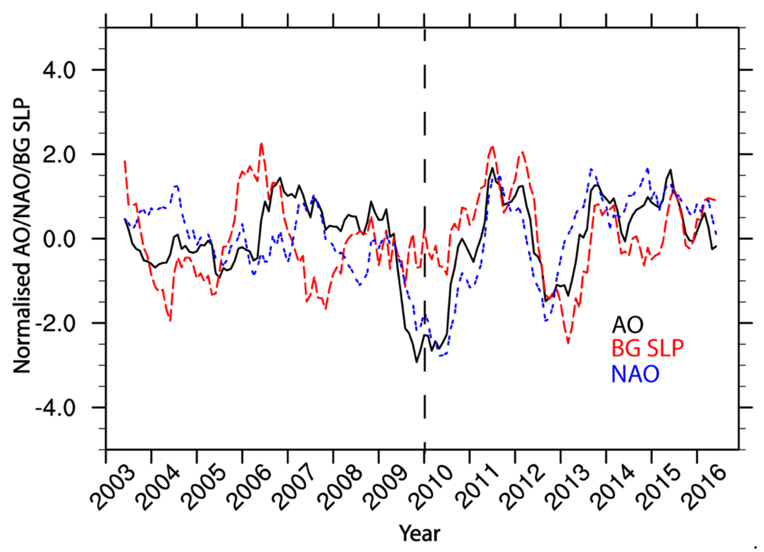
2.4. Atmospheric Variables

The atmospheric variables including sea level pressure (SLP), turbulent (sensible and latent) heat fluxes at the air–sea interface, and surface air temperature is obtained from ECMWF-ERA5 [48] datasets with a grid resolution of 0.25 × 0.25 deg. The monthly anomalies are calculated based on 1979–2017 climatology. Moreover, the monthly indices of North Atlantic Oscillation (NAO) [49] and Arctic Oscillation (AO) [50] are obtained from https://www.cpc.ncep.noaa.gov/.

2.5. Trend Analysis

We analyze the time series using a least-squares joint adjustment of a multiparameter fit function to the observables. This includes terms for offset, slope and semi-annual and annual cosine and sine cycles, respectively. The linear term (slope) of the resulting fit function is taken as a linear trend. For detrending and reduction of semi-/annual cycles, the corresponding terms of the fitted function are removed from the observable, respectively, and subsequently undergoing correlation analyses. Uncertainties in the sea level trend from altimetry are shown as the 2.5% percentile (Figure 1b) and the 97.5% percentile (Figure 1c) corresponding to the 95% confidence level.

3. Results

3.1. Altimeter Sea Level

The spatial trend (2003–2016) in the altimeter derived sea level data of the Arctic Ocean is shown in Figure 1a. The figure shows three regions where the trend is distinctly positive, notably: BG; NS; and the Barents Sea. Of the three, BG is the largest freshwater reservoir (above 65°N) [51], while NS is the largest heat reservoir in the Arctic domain [52]. Note that the total area of the NS and BG is much larger than the total area of the Barents Sea, which is a shelf sea (average depth around 250 m). Hence, we restrict our focus to NS and BG. Furthermore, it is well-known that while BG plays a flywheel role and stabilizes the climate of the entire Arctic [53], the heat transported from the North Atlantic into NS impacts the regional climate [54]. A positive sea level trend in NS and BG can be due to changes in heat and freshwater contents in these regions. An opposite trend in the sea level is found in the Baffin Bay and the Russian Sector of the Arctic, also a shelf region (less than 500 m depth). All in all, the Arctic Ocean is a region where the sea level shows both positive and negative trends during the altimeter era.
Figure 2 shows the monthly variability in the sea level of the BG and the NS. From a closer inspection of the monthly variability, it is evident that the entire time series can be divided into two seven-year time periods (first time period (T1), 2003–2009; second time period (T2), 2010–2016), where the sea level trend of the two regions is different. A substantial increase in the sea level of BG (9.7 mm/yr) is noted during T1, while the trend is opposite in NS (−2.8 mm/yr). In contrast, the sea level trend in BG weakens (2.4 mm/yr), while a substantial increase is found in NS (9.7 mm/yr) during T2. In this study, moreover, we found an on-and-off coherence between the sea level variability in BG and NS during T2 and T1. While a strong correlation (r = 0.73) between the monthly detrended time series of the two regions is found during T2, there is no evidence of this correlation during T1 (r = 0.1). Notably, the high correlation between the two time series during T2 is dominated by the coherence in their seasonality. As a result, the deseasoned and detrended correlation between the two-time series during T2 is much less (r = 0.31).
We hypothesize, that the change in sea level variability of the two regions and the on-and-off coherence during the study period could be linked to the variability in the dominant large-scale atmospheric circulations over the Arctic. This argument is further supported by Figure 3 which shows a change in the large-scale atmospheric circulation pattern over the Arctic during T1 and T2. Arctic Oscillation (AO) [50] and Arctic Dipole (AD) are the two dominant large-scale atmospheric circulation features of the Arctic [55]. While AO features as a pan Arctic SLP variability, AD is characterized by an east–west dipole in SLP over the Arctic. Figure 3 shows that while the AD pattern dominates the atmospheric variability over the Arctic during T1, the AO pattern dominates during T2. In short, our analysis (Figure 2 and Figure 3) suggests that the analysis of sea level budget analysis of the Arctic Ocean during GRACE/Argo time period (2003–2016) should be split into two separate time periods centered around the year 2010, in order to capture the impact of the apparent shift in the long-term pattern of the SLP. Here, it should be noted that year 2010, marks the launch of the Cryosat-2 mission. As such, the DTU/TUM SLA contains in the period from November 2010 to March 2012 a combination of Envisat and CryoSat, while after March 2012 the data record solemnly contains CryoSat-2 data. This may have had an impact on the sea level time series over the BG.
The sea level trend in the Arctic during T1 and T2 is shown in Figure 4. A distinct high positive sea level trend is found in the BG during T1 in consistence with the time series shown in Figure 2. Negative trends are found in Baffin Bay, NS and near the northern Barents Sea (Figure 4a). During T2, the positive sea level trend in the BG has flattened, while it is much more prominent in the NS, the northern area of the Bering Strait and the Barents Sea (Figure 4b).

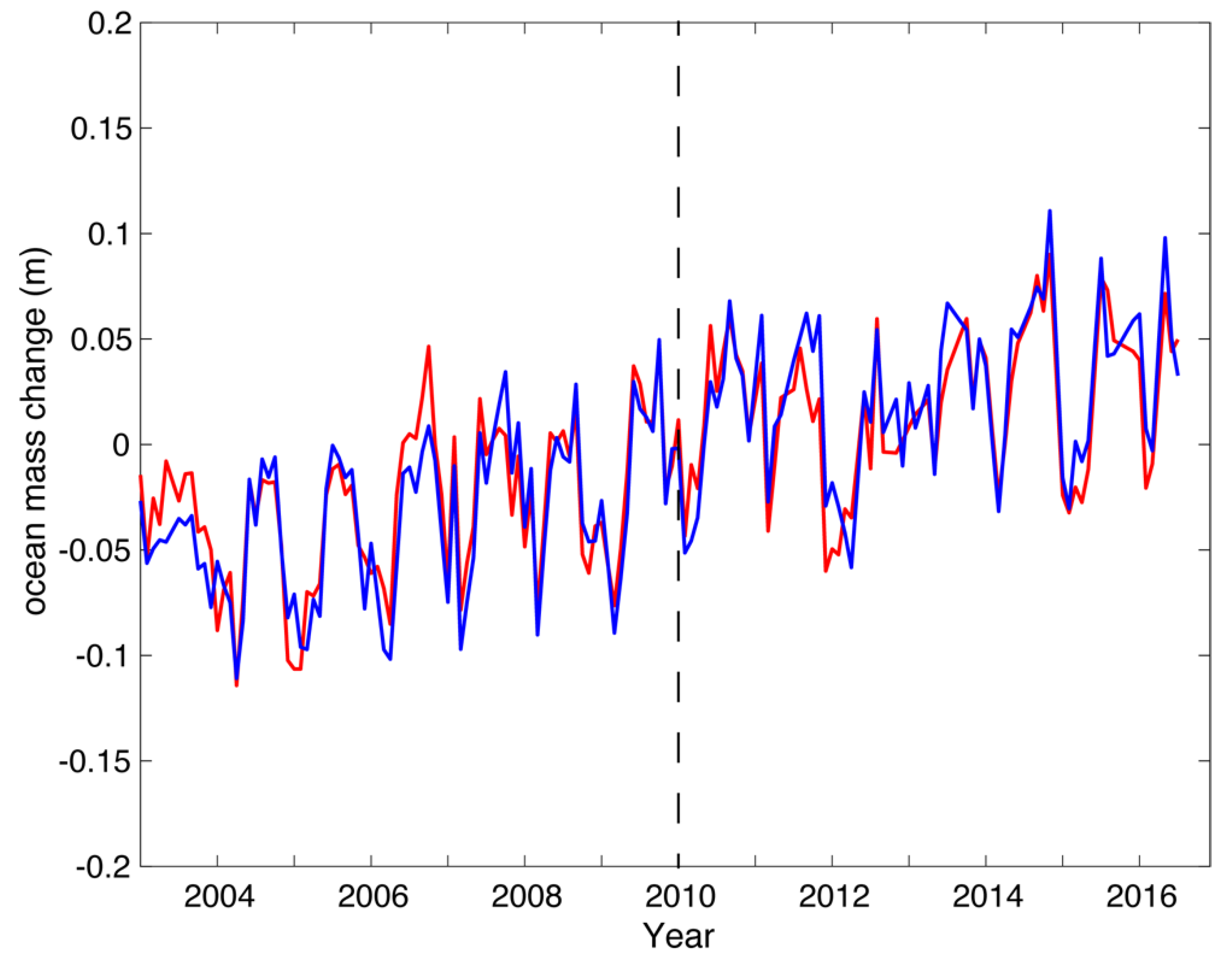
3.2. Ocean Mass Change

Ocean mass changes over the Arctic during T1 and T2 are shown in Figure 5. In general, the GSFC Mascon product shows a positive trend in the Arctic, except for over the northern Barents Sea (Figure 5a,b) and in Baffin Bay (Figure 5b). Trends over BG and NS are also positive, with no substantial change in their respective trends during the two time periods T1 (BG, 6.0 mm/yr; NS, 5.0 mm/yr) and T2 (BG, 6.8 mm/yr; NS, 4.9 mm/yr). However, a notable trend reversal is found in the Baffin Bay during T1 and T2. In comparison, one notices the very low spatial coverage derived from the SH solutions (after masking the polar gap) shown in Figure 5c,d. This is due to the fact that SH solutions cannot include areas close to the coast (~300 km) as they would include leakage of mass change signals from the continents. On the other hand, the remaining spatial patterns shown in SH solution are comparable to the mascon-based results.
Next, we focus on the monthly ocean mass variability in BG and NS (Figure 6). The time series analysis of the ocean mass change in BG and NS shows a profound similarity. A very high correlation (r = 0.9) is found between the detrended monthly time series for the two regions during both T1 and T2. After removing the annual and semiannual cycle and after detrending, the analyses provide the same result indicating a high level of coherence between the ocean mass variability of the two regions (r = 0.82, in both T1 and T2).

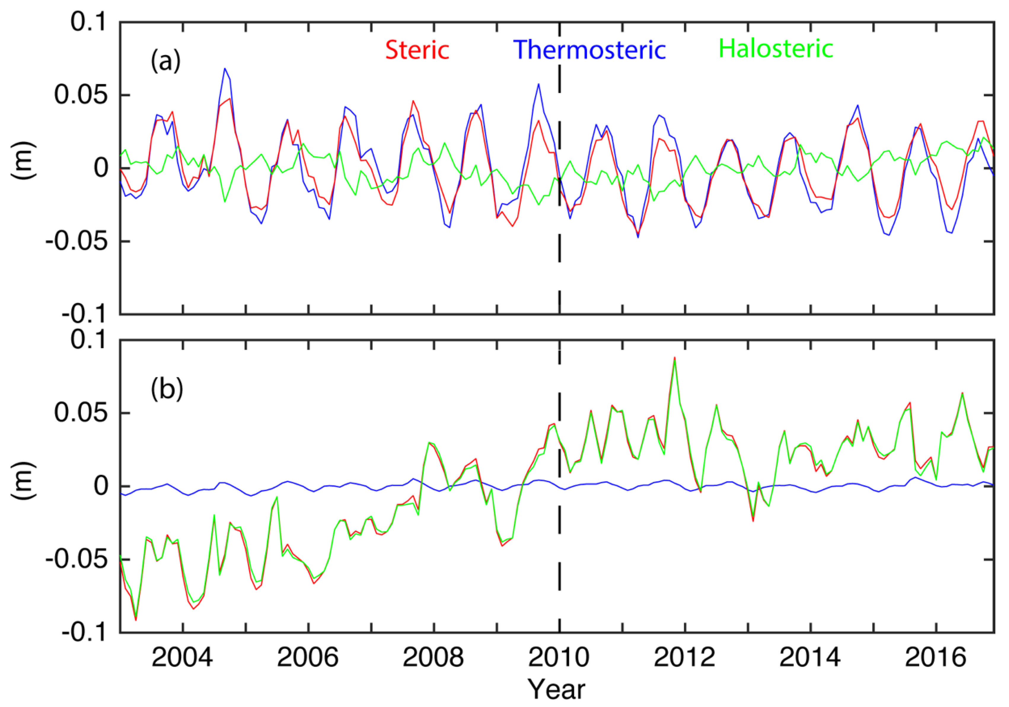
3.3. Steric Sea Level Variability

The linear trends in the steric sea level height and its components (thermosteric and halosteric) during T1 and T2 are shown in Figure 7. During T1, the positive trend in the steric sea level height is found to be the largest in BG (Figure 7a). During the same time period negative trends are noted over the Russian shelf region. On the other hand, during T2, the largest positive trend is found over NS, while a considerable weakening of the positive trend is noted over BG (Figure 7b). The trends in thermosteric sea level during T1 and T2 are shown in Figure 7c,d. The trend is notably positive in thermosteric sea level in NS, especially in its northern part during T2, while the overall trend seems to be more on the negative side during T1. It is also interesting to note the strong negative values in the southern part of the NS during T2. A closer inspection also shows patches in the eastern part where the trend is negative. Unlike NS, over BG, no notable change is depicted in the thermosteric sea level trend during the two time periods, while distinct trends in the halosteric sea level are found both during T1 and T2 as seen in Figure 7e,f. The positive value in the steric sea level height in BG during T1 and its weakening during T2 therefore can be explained by the increase/weakening in the halosteric sea level component. The negative trend in steric sea level trend encountered in the Russian shelf region during T1, moreover, is also likely due to the same effect.
The steric sea level variability in the NS also seems to be affected by the halosteric component especially near Svalbard and also in the southern part. During T2, while the trend is negative near Svalbard, it is highly positive towards the southern part. The slightly negative trend in steric sea level height during T2 in the southern part of the NS is the result of balance in the positive halosteric component (positive) and the highly negative thermosteric component.
The monthly variability (anomalies) of the steric sea level and its components averaged over NS and BG are shown in Figure 8. In NS, there is a very close alignment between the steric sea level height and the thermosteric component. The figure also shows a clear seasonality in the steric sea level height and its component. Notably the weaker halosteric component of the sea level is in the opposite phase of the thermosteric component, indicating the huge impact of the warm and saline Atlantic Water in determining the steric sea level variability of NS. The overall trend in steric sea level in NS is positive during T2 (1.6 mm/yr), while it is negative during T1 (−2.3 mm/yr). Notably the thermosteric trend is negative during both time periods (T1, −0.2 mm/yr; T2, −1.7 mm/yr). The halosteric component, on the other hand, is negative during T1 (−2.1 mm/yr) while it is positive during T2 (3.3 mm/yr). The authors of [56] reported a freshening in the Norwegian Sea (eastern Nordic Seas) during T2, and the results shown in Figure 7e, f and Figure 8a are consistent with their findings. We argue that the positive trends in both the halosteric sea level and the ocean mass change results in the steep rise of the sea level in NS during T2. On the contrary, the halosteric and ocean mass change trends are of opposite signs during T1, which may have resulted in the weakening of the trend.
In the case of BG, the steric height variability is fully dominated by the halosteric sea level (Figure 8b). While there is a strong positive trend in the steric sea level during T1 (11.4 mm/yr), the trend weakens considerably during T2 (−1.0 mm/yr). This is in accordance with the respective increase and decrease in the halosteric sea level during T1 (10.8 mm/yr) and T2 (−1.0 mm/yr). The thermosteric variability (anomaly) during the entire time period is fluctuates around zero, i.e., there is no major change in it from its mean value. Accordingly, the thermosteric sea level trend during both time periods is much smaller (T1, 0.6 mm/yr; T2, 0.01 mm/yr). Note that the trend in ocean mass change in BG during both time periods shows an increasing trend (Figure 6) and does not follow the behavior of sea level trend during T2 (Figure 2). Hence it can be argued that the trend in sea level variability of BG is controlled by the change in the halosteric sea level of the region, which shows both the increasing trend during T1 and the stabilization phase during T2 where the trend flattens.

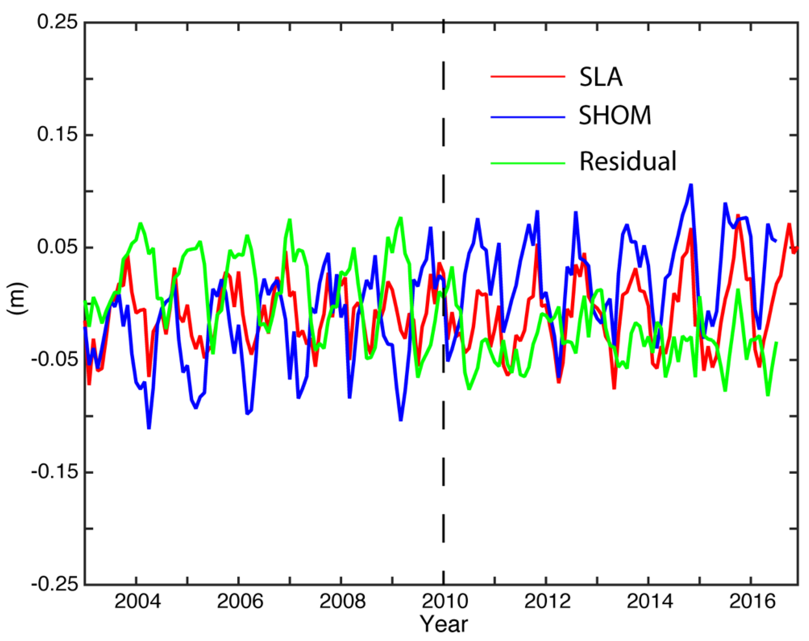
3.4. Arctic Sea Level Budget Assessment

Ideally, the closure of the Arctic sea level budget implies that the observed changes in the sea level as determined from satellite altimetry equal the sum of observed changes in ocean mass and the steric height. Figure 9 shows the comparison of the variability in the altimeter derived sea level of the entire Arctic Ocean (area shown in Figure 1) to the sum of observed changes in steric sea level height and ocean mass change (termed as ‘SHOM’ for simplicity). The monthly variability of SLA and SHOM averaged over the Arctic region during the 14-year time period are found to be within −0.1 to 0.1 m. An interesting finding is the similarity (in-phase) in the seasonality of altimeter sea level and SHOM during T2, which is not the case in T1. The correlation (detrended) between the two is higher during T2 (r = 0.76) in comparison to T1 (r = 0.42). Furthermore, the amplitude of the residual time series is also reduced by nearly half during T2 in comparison to T1.
Sea level budget assessment for the entire Arctic based on trend values is summarized in Table 1. The trend in altimeter derived sea level during T2 (4.0 mm/yr) is higher than T1 (1.0 mm/yr). On the other hand, even though not of the same magnitude, the trend in SHOM is also higher during T2 (5.0 mm/yr) than T1 (4.2 mm/yr). Our analysis was not able to close the sea level budget of the Arctic, as there is a considerable residual trend during both T1 (−3.2 mm/yr) and T2 (−1.0 mm/yr). Two sub-regional sea level budget analyses were also performed, one in NS (Table 2), and the other in BG (Table 3). In BG, the residual trend is –10.0 mm/yr during T1, while it is much lower during T2 (−3.6 mm/yr). In comparison, in NS, it is −3.0 mm/yr during T1 and −0.9 mm/yr during T2.

4. Discussion

Our study examined the sea level variability of the Arctic Ocean which is experiencing the most severe impacts of climate change during the recent decades. Analysis found two major regions in the Arctic Ocean with positive sea level trends (Figure 1) during the GRACE/Argo period (2003–2016). In BG, a steep rise in sea level is noted during T1, followed by a stabilization phase in T2 where the trend flattens (Figure 2). The intensification and stabilization phase of the BG sea level variability respectively during T1 and T2, has been reported in previous studies [13,57]. The difference in the BG sea level trend during T1 and T2 can be linked to the change in dominant atmospheric forcing over the Arctic during the two time periods as seen in Figure 3. The large-scale atmospheric pattern during T1 depicts an Arctic dipole pattern, the second mode of variability in the Arctic with a high pressure over the western Arctic and low pressure over eastern Arctic. The dominance of the AD during T1 (Figure 3a) maintained the BH, a semi-permanent atmospheric circulation pattern, which is well-known to drive the anticyclonic circulation of BG [58]. The resulting Ekman convergence stores the sea-ice and fresh water in the region. The piling up of freshwater in the BG contributes to halosteric changes in sea-level [59,60] and resulted in a rise of the sea level [61]. This is in line with other works in the literature which, investigating salinity-induced sea-level variations, underline the connection between ocean freshening and sea-level rise [62,63], and are in accordance with our results over BG (Figure 2 and Figure 8b). During T2, the dominant forcing over the Arctic changes to AO (Figure 3b). The high coherence of BG SLP with AO and NAO during T2 (Figure 10) further supports our findings. The correlation between AO and BG SLP are higher during T2 (interannual, r = −0.6) in comparison to T1 (interannual, r = −0.2). The negative correlation between AO and BG SLP, also seen in Figure 10, indicates the weakening of BH in association with AO. The change from AD to AO during T2 thus results in the break in the piling of fresh water in BG and as a result, the rapid rise in sea level ceases (Figure 2) which leads to a stabilization period where the sea level trend of the region flattens out. This is further confirmed by the trend in the halosteric steric sea level which also flattens during T2 (Figure 8b).
The findings of this study also highlight the possibility of inferring the trend in BG sea level based on the dominant large-scale atmospheric forcing over the Arctic. It is well-known that making regional sea level projections is a challenge, since several processes relevant for sea level are not adequately represented in climate models [4]. Understanding the relevant physical mechanisms associated with Arctic climate variability is expected to improve model projections of sea level by examining the ability of the climate models to replicate observed features and processes. This gives insight into their suitability for projecting sea level rise and allows for weighting or eliminating models from the ensemble if they fail to adequately reproduce the observations, thus narrowing the uncertainty and improving confidence [64].
Next we focus on the role of a change in dominant atmospheric forcing over the Arctic on the sea level variability of NS. Our study reveals the coherence in the sea level variability of BG and NS during T2 (Figure 2), as well as the higher coherence between AO and NAO (Figure 10). The correlation analysis confirms the higher coherence between NAO, the dominant atmospheric forcing over the Nordic Seas [65,66], and AO during T2 (interannual, r = 0.9) than during T1 (interannual, r = 0.5). The close relation and the nearly indistinguishable nature [65] of AO and NAO is more prominent during T2. A change in atmospheric forcing over the Arctic can impact the sea level in NS, both directly and indirectly. The direct effect is via the variability in the sea ice export from the Arctic into NS and its subsequent impact on the steric sea level height. The indirect effects are associated with a possible change in the atmospheric variability over NS in association with a change in dominant atmospheric forcing over the Arctic and the subsequent impact on the sterodynamic [67] sea level of the region (indirect effect). This in particular is relevant due to the impact of atmospheric variability on: (a) the Atlantic Water (AW) transport into NS [68,69] which influences the steric sea level [56]; (b) the slope current in the eastern NS [52,70,71,72] that in turn can result in the decoupling [73] of the open ocean sea level rise redistributed (mass redistribution) onto shelf areas of the Norwegian coast (known as shelf mass loading, see [74]); and (c) on waves in the NS [75] which may also impact the sea level, as has been found in [76]. Careful analyses of these three points is out of the scope of this paper.
Another interesting finding of this study is the similarity (in-phase) in the seasonality of altimeter sea level and the sum of the observed changes in steric sea level height and ocean mass change over the Arctic domain (Figure 9) during T2, which is not found during T1 (Figure 9). This is found to be linked to a much well-defined seasonal cycle in the Arctic sea level during T2 in comparison with T1. At this stage, however, it is not clear how this difference in seasonality can be linked to atmospheric forcing. Furthermore, it should also be noted that the Cryosat-2 altimeter mission was launched in 2010 and this altimeter data has been incorporated into the sea level product since November 2010 (T2). It needs to be understood how Cryosat-2 data influences the retrieval of sea level variability of the Arctic region from satellite altimetry. With CryoSat-2 we have a new satellite altimeter capable of capturing the leads in-between the sea-ice floes with a much higher precision. The satellite orbit and repeat cycle (369 days) also resulted in much better spatial data coverage in the Arctic Ocean than ever before, leading to an SLA record with a lower uncertainty [14]. A detailed analysis is needed in the future to differentiate between the effect of conventional altimetry (LRM) to SAR/SARIn altimetry (in T1/T2) and the role of atmospheric forcing during the two time periods. It is also not clear if the annual and inter-annual changes of the CryoSat-2 mode mask plays a role in the altimetric SLA, and what the consequences are of not using sea state bias in SAR/SARIn mode in the sea ice marginal zone [20]. This is currently been investigated.
The Sea-level budget assessment analysis is done for the entire Arctic and for the two subregions, BG and NS. Analysis found considerable residual trends during both time periods, the lowest during T2 (0.9 mm/yr). The nonclosure of the sea level budget in the Arctic is expected since all three datasets in use have limitations in the Arctic region.
(1) The retrieval accuracy in the altimetric dataset is, in particular, questioned with respect to: (a) Retrievals of summer waveform data whereby melting sea-ice and melt ponds can mistakenly be evaluated as leads giving too high SLAs and hence a too low sea level trend; (b) Retracking challenges in the marginal ice zones where the presence of waves can influence the sea level estimates. For this reason, the need for using a physical retracker, where the possibility of retrieving the sea state bias, is crucial for the complete SLA record.
(2) The concern regarding the steric height estimates, arises from the poorly observed interior Arctic Ocean in space and time implying that uncertainties may creep in due to heavy interpolation-driven smoothing.
(3) For the ocean mass change data, our study was not able to benefit from unconstrained SH-solutions for the ocean mass changes due to low spatial resolution and coverage after leakage-buffering and removal. A possible alternative may be the development of a new tailored-kernel solution for ocean mass change from GRACE data, based on an approach by [76] that has already been utilized for Antarctica.

5. Conclusions

The Arctic Ocean is a region experiencing the most rapid climate change during the recent decades. One of the aims of the ESA’s Sea level Budget Closure project is to provide the sea level budget assessment of the Arctic Ocean using newly reprocessed satellite altimeter data, newly estimated GRACE derived ocean mass changes and steric height estimates. Trend analysis of the altimeter data showed regions with both positive and negative trends in the Arctic Ocean. The Beaufort Gyre and the Nordic Seas are the two regions with positive trends in the Arctic during the full GRACE/Argo period (2003–2016). Altimeter derived sea level in these regions reveals a significant shift in the trend pattern around 2009–2011. In BG, there is a steep rise in sea level during the first period (T1; 2003–2009), followed by a stabilization phase in the second period (T2, 2010–2016) where the trend flattens. On the other hand, in NS there is a negative trend during the first period followed by a strong positive trend. Further analysis suggests that this shift, especially over BG, can be explained by a change in large-scale atmospheric circulation pattern over the Arctic. Evidence of AO as the major driver of pan Arctic SLP variability during 2010–2016 is presented. The similarity between sea level trend and halosteric height trend further confirms the link between fresh water and sea level variability in BG. Our results highlight the possibility of predicting BG sea level based on the dominant atmospheric forcing over the Arctic.
We further reveal the coherence in the sea level variability of NS and BG during 2010–2016 (T2), as well as the coherence between AO, BG SLP and NAO over the same period. We summarize the direct and different indirect effects of the atmospheric variability over NS on the sea level there and recommend a separate study to investigate them in detail. Our analysis also found a profound similarity between the variability in the ocean mass of BG and NS. From the trends of ocean mass change and steric sea level height and its components, we hypothesize that the steep increase in NS sea level during 2010–2016 (T2), is likely due to the combined effect of ocean mass change and halosteric sea level trend.
Another interesting result is the similarity (in-phase) in the seasonality of altimeter sea level and SHOM (sum of ocean mass change and steric height) of the Arctic appearing only during the second period. We point to the possible role of the availability of Cryosat-2 altimeter data and recommend a future study to analyze the effect of change in conventional altimetry to SAR/SARIn altimetry on the retrieval of sea level variability in these two periods. The latter could also help to explain the large differences observed when comparing sea-level budget assessments (based on trend values; e.g., Table 1) over the two analysis sub-periods.
The Sea-level budget assessment of the entire Arctic and in BG and NS sub-regions for the two time periods shows a residual trend of more than 0.9 mm/yr, indicating a nonclosure of the sea level budget. This nonclosure of the sea level budget is further attributed to the limitations of the satellite altimeter data, ocean mass change data and steric height estimates in the Arctic region and are detailed. Recommendations for further studies therefore include:
(i) Improved summer retrievals in sea ice covered areas from satellite altimetry by gaining better understanding of the radar altimeter response over the different ice types;
(ii) Improve estimation of the steric component through incorporation of more/all-available in-situ observations with better coverage;
(iii) Update the ocean mass change data using state-of-the-art solutions, for example by using the new Global tailored-kernel solutions based on [76], with higher resolution and including leakage-regions near the coast as well.
Finally, we highlight the immediate need for various national and international organizations to intensify their efforts in increasing the number of geodetically connected tide gauges in the Arctic. The altimeter data used in this study has been validated by [20] using six tide gauges spread along the coast in the Arctic Ocean. They did not find a good correlation in the Russian Sector of the Arctic, even though the correlation at other locations were very high. They attributed it to bad data coverage, vertical land movement, and/or outflow from large rivers. Previous attempts to validate altimetric sea level in the Arctic using tide gauges also found a similar spatial pattern of difference in correlation values [13,77]. Those studies also found a smaller correlation between altimeter data and tide gauge data in the Russian side of the Arctic, for example in the Kara, Laptev and East Siberian Seas. In brief there is an immediate need to reduce the sparseness of available stations in the Arctic which is clearly inhibiting reliable analyses of local variabilities and trends in comparison to the satellite observations. The relevance is further highlighted in Figure 1, which shows that the sea level variability over the Arctic is not uniform but differs spatially. Furthermore, the necessity is even higher in the present era where we experience strong mass losses from ice sheets and glaciers around the Arctic, which in combination with isostatic adjustment is expected to result in the fall of sea level in its immediate vicinity, while central parts of the ocean undergo relative accumulation of water masses [78,79] thereby increasing the regional difference in sea level. Finally, the shallow shelves bordering the Arctic Ocean are expected to gain mass from a redistribution of sea water from the interior oceans, leading to self-attraction and loading effects that may result in an even higher sea level rise [73].

Author Contributions

Conceptualization, ESA CCI SLBC project team (H.P., C.A.L., L.B., P.K., A.H., A.C.); methodology, ESA CCI SLBC project team (H.P., C.A.L., L.B., P.K., A.H., A.C.); software, B.D.G., J.E.Ø.N.; formal analysis, R.P.R., S.C.; investigation, R.P.R., S.C., B.D.G.; resources, O.B.A., S.K.R., H.R., B.D.G., M.H.; writing—original draft preparation, R.P.R.; writing—review and editing, R.P.R., S.C., B.D.G., A.B., K.R., J.A.J. and the ESA CCI SLBC project team (H.P., C.A.L., L.B., P.K., A.H., A.C.); supervision, J.A.J., O.B.A.; project administration, M.H.; funding acquisition, J.B. All authors have read and agreed to the published version of the manuscript.

Funding

This research was funded by ESA Climate Change Initiative Sea level Budget Closure, contract No. 4000119910/17/I-NB. Additional funding for the manuscript preparation has been provided by the Center for Climate Dynamics CHEX project and Bjerknes Center Fast track Initiative.

Acknowledgments

First author Raj acknowledges the in-kind funding from the Nansen Environmental Remote Sensing Center, and also S. H. Mernild for his support. Chatterjee acknowledges Nansen Scientific Society for the support.

Conflicts of Interest

The authors declare no conflict of interest.

References

  1. IPCC. Climate Change 2013. In The Physical Science Basis; Cambridge University Press: Cambridge, UK, 2013; p. 1535. [Google Scholar]
  2. Horwath, M.; Novotny, K.; Cazenave, A.; Palanisamy, H.; Marzeion, B.; Paul, F.; Döll, P.; Cáceres, D.; Hogg, A.; Shepherd, A.; et al. ESA Climate Change Initiative (CCI) Sea Level Budget Closure (SLBC_cci) Executive Summary Report D4.4; Version 1.0; ESA: Rome, Italy, 2020. [Google Scholar]
  3. Von Schuckmann, K.; Palmer, M.D.; Trenberth, K.E.; Cazenave, A.; Chambers, D.; Champollion, N.; Hansen, J.; Josey, A.S.; Loeb, N.; Mathieu, P.-P.; et al. Earth’s energy imbalance: An imperative for monitoring. Nat. Clim. Chang. 2016, 26, 138–144. [Google Scholar] [CrossRef] [Green Version]
  4. Church, J.; Clark, P.; Cazenave, A.; Gregory, J.; Jevrejeva, S.; Levermann, A.; Merrifield, M.; Milne, G.; Nerem, R.; Nunn, P.; et al. Sea level change. In Climate Change 2013: The Physical Science Basis; Contribution of Working Group I to the Fifth Assessment Report of the Intergovernmental Panel on Climate Change; PM Cambridge University Press: Cambridge, UK, 2013; pp. 1137–1216. [Google Scholar]
  5. WCRP Global Sea Level Budget Group. Global sea-level budget 1993–present. Earth Syst. Sci. Data 2018, 10, 1551–1590. [Google Scholar] [CrossRef] [Green Version]
  6. Oppenheimer. Sea Level Rise and Implications for Low Lying Islands, Coasts and Communities Chapter 4: Sea Level Rise and Implications for Low Lying Islands, Coasts and Communities’; IPCC Special Report on the Ocean and Cryosphere in a Changing Climate; Pörtner, H.-O., Ed.; Cambridge University Press: Cambridge, UK, 2019. [Google Scholar]
  7. Dieng, H.; Cazenave, A.; Meyssignac, B.; Ablain, M. New estimate of the current rate of sea level rise from a sea level budget approach. Geophys. Res. Lett. 2017, 44, 3744–3751. [Google Scholar] [CrossRef]
  8. Legeais, J.F.; Ablain, M.; Zawadzki, L.; Zuo, H.; Johannessen, J.A.; Scharffenberg, M.G.; Fenoglio-Marc, L.; Fernandes, M.J.; Andersen, O.B.; Rudenko, S.; et al. An improved and homogeneous altimeter sea level record from the ESA Climate Change Initiative. Earth Syst. Sci. Data 2018, 10, 281–301. [Google Scholar] [CrossRef] [Green Version]
  9. Frederikse, T.; Landerer, F.; Caron, L.; Adhikari, S.; Parkes, D.; Humphrey, V.W.; Dangendorf, S.; Hogarth, P.; Zanna, L.; Cheng, L.; et al. The causes of sea-level rise since 1900. Nature 2020, 584, 393–397. [Google Scholar] [CrossRef] [PubMed]
  10. Stammer, D.; Cazenave, A.; Ponte, R.M.; Tamisiea, M.E. Causes for contemporary regional sea level changes. Annu. Rev. Mar. Sci. 2013, 5, 21–46. [Google Scholar] [CrossRef] [Green Version]
  11. Carret, A.; Johannessen, J.A.; Andersen, O.B.; Ablain, M.; Prandi, P.; Blazquez, A.; Cazenave, A. Arctic Sea Level During the Satellite Altimetry Era. Surv. Geophys. 2017, 38, 251–275. [Google Scholar] [CrossRef]
  12. Proshutinsky, A.; Ashik, I.M.; Dvorkin, E.N.; Häkkinen, S.; Krishfield, R.A.; Peltier, W.R. Secular sea level change in the Russian sector of the Arctic Ocean. J. Geophys. Res. Oceans 2004, 109, C03042. [Google Scholar] [CrossRef]
  13. Armitage, T.W.K.; Bacon, S.; Ridout, A.L.; Thomas, S.F.; Aksenov, Y.; Wingham, D.J. Arctic sea surface height variability and change from satellite radar altimetry and GRACE, 2003–2014. J. Geophys. Res. Oceans 2016, 121, 4303–4322. [Google Scholar] [CrossRef] [Green Version]
  14. Rhein, M.; Rintoul, S.R.; Aoki, S.; Campos, E.; Chambers, D.; Feely, R.A.; Gulev, S.; Johnson, G.C.; Josey, S.A.; Kostianoy, A.; et al. Observations: Ocean; Climate Change 2013: The physical science basis. In Contribution of Working Group I to the Fifth Assessment Report of the Intergovernmental Panel on Climate Change; Stocker, T.F., Qin, D., Plattner, G.-K., Tignor, M., Allen, S.K., Boschung, J., Nauels, A., Xia, Y., Bex, V., Midgley, P.M., Eds.; Cambridge University Press: Cambridge, UK, 2013. [Google Scholar]
  15. Stroeve, J.C.; Kattsov, V.; Barrett, A.; Serreze, M.; Pavlova, T.; Holland, M.; Meier, W.N. Trends in Arctic sea ice extent from CMIP5, CMIP3 and observations. Geophys. Res. Lett. 2012, 39, L16502. [Google Scholar] [CrossRef] [Green Version]
  16. Proshutinsky, A.; Dukhovskoy, D.; Timmermans, M.L.; Krishfield, R.; Bamber, J.L. Arctic circulation regimes. Philos. Trans. R. Soc. A 2015, 373, 20140610. [Google Scholar] [CrossRef] [PubMed] [Green Version]
  17. Tedesco, M.; Doherty, S.; Fettweis, X.; Alexander, P.; Jeyaratnam, J.; Stroeve, J. The darkening of the Greenland ice sheet: Trends, drivers and projections (1981–2100). Cryosphere 2016, 10, 477–496. [Google Scholar] [CrossRef] [Green Version]
  18. Fritz, M.; Vonk, J.; Lantuit, H. Collapsing Arctic coastlines. Nat. Clim. Chang. 2017, 7, 6–7. [Google Scholar] [CrossRef] [Green Version]
  19. Jones, B.M.; Arp, C.D.; Jorgenson, M.T.; Hinkel, K.M.; Schmutz, J.A.; Flint, P.L. Increase in the rate and uniformity of coastline erosion in Arctic Alaska. Geophys. Res. Lett. 2009, 36, L03503. [Google Scholar] [CrossRef]
  20. Rose, S.K.; Andersen, O.B.; Passaro, M.; Ludwigsen, C.A.; Schwatke, C. Arctic Ocean Sea Level Record from the Complete Radar Altimetry Era: 1991–2018. Remote Sens. 2019, 11, 1672. [Google Scholar] [CrossRef] [Green Version]
  21. Passaro, M.; Rose, S.; Andersen, O.; Boergens, E.; Calafat, F.; Dettmering, D.; Benveniste, J. ALES+: Adapting a homogenous ocean retracker for satellite altimetry to sea ice leads, coastal and inland waters. Remote Sens. Environ. 2018, 211, 456–471. [Google Scholar] [CrossRef] [Green Version]
  22. Andersen, O.B.; Piccioni, G. Recent Arctic Sea Level Variations from Satellites. Frontiers in Marine Science 2016, 3, 76. [Google Scholar] [CrossRef] [Green Version]
  23. Johannessen, J.; Andersen, O. The High Latitudes and Polar Ocean; CRC Press: Boca Raton, FL, USA, 2017. [Google Scholar]
  24. Ludwigsen, C.A.; Andersen, O.B. Contributions to Arctic sea level from 2003 to 2015. Adv. Space Res. 2019, in press. [Google Scholar] [CrossRef]
  25. Cheng, Y.; Andersen, O.B. Multimission empirical ocean tide modeling for shallow waters and polar seas. J. Geophys. Res. Oceans 2011, 116, 1–11. [Google Scholar] [CrossRef] [Green Version]
  26. Cheng, Y.; Andersen, O.B.; Knudsen, P. An Improved 20-Year Arctic Ocean Altimetric Sea Level Data Record. Mar. Geod. 2015, 38, 146–162. [Google Scholar] [CrossRef]
  27. Prandi, P.; Ablain, M.; Cazenave, A.; Picot, N. A New Estimation of Mean Sea Level in the Arctic Ocean from Satellite Altimetry. Mar. Geod. 2012, 35, 61–81. [Google Scholar] [CrossRef] [Green Version]
  28. Tapley, B.D.; Bettadpur, S.; Watkins, M.; Reigber, C. The gravity recovery and climate experiment: Mission overview and early results. Geophys. Res. Lett. 2004, 31, L09607. [Google Scholar] [CrossRef] [Green Version]
  29. Raj, R.P. Surface velocity estimates of the North Indian Ocean from satellite gravity and altimeter missions. Int. J. Remote Sens. 2017, 38, 296–313. [Google Scholar] [CrossRef]
  30. Landerer, F.W.; Flechtner, F.M.; Save, H.; Webb, F.H.; Bandikova, T.; Bertiger, W.I.; Bettadpur, S.V.; Byun, S.H.; Dahle, C.; Dobslaw, H.; et al. Extending the global mass change data record: GRACE Follow-On instrument and science data performance. Geophys. Res. Lett. 2020, 47, e2020GL088306. [Google Scholar] [CrossRef]
  31. Luthcke, S.B.; Sabaka, T.J.; Loomis, B.D.; Arendt, A.A.; McCarthy, J.J.; Camp, J. Antarctica, Greenland and Gulf of Alaska land ice evolution from an iterated GRACE global mascon solution. J. Glaciol. 2013, 59, 613–631. [Google Scholar] [CrossRef]
  32. Kvas, A.; Behzadpour, S.; Ellmer, M.; Klinger, B.; Strasser, S.; Zehentner, N.; Mayer-Gürr, T. ITSG-Grace2018: Overview and evaluation of a new GRACE-only gravity field time series. J. Geophys. Res. Solid Earth 2019, 124, 9332–9344. [Google Scholar] [CrossRef] [Green Version]
  33. Swenson, S.; Chambers, D.; Wahr, J. Estimating geocenter variations from a combination of GRACE and ocean model output. J. Geophys. Res. Solid Earth 2008, 113, B08410. [Google Scholar] [CrossRef] [Green Version]
  34. Cheng, M.K.; Ries, J.C. The unexpected signal in GRACE estimates of C20. J. Geod. 2017, 91, 897–914. [Google Scholar] [CrossRef]
  35. Cheng, M.K.; Tapley, B.D.; Ries, J.C. Deceleration in the Earth’s oblateness. J. Geophys. Res. 2013, V118, 1–8. [Google Scholar] [CrossRef]
  36. Wahr, J.; Nerem, R.S.; Bettadpur, S.V. The pole tide and its effect on GRACE time-variable gravity measurements: Implications for estimates of surface mass variations. JGR Solid Earth 2015, 120, 4597–4615. [Google Scholar] [CrossRef]
  37. Flechtner, F.; Dobslaw, H.; Fagiolini, E. AOD1B Product Description Document for Product Release 05, GRACE 327-750 (GR-GFZ-AOD-0001), GFZ German Research Centre for Geosciences; Department 1: Geodesy and Remote Sensing; GFZ: Potsdam, Germany, 2014. [Google Scholar]
  38. Dobslaw, H.; Bergmann-Wolf, I.; Dill, R.; Poropat, L.; Thomas, M.; Dahle, C.; Esselborn, S.; König, R.; Flechtner, F. A New High-Resolution Model of Non-Tidal Atmosphere and Ocean Mass Variability for De-Aliasing of Satellite Gravity Observations: AOD1B RL06. Geophys. J. Int. 2017, 211, 263–269. [Google Scholar] [CrossRef] [Green Version]
  39. Geruo, A.; Wahr, J.; Zhong, S. Computations of the viscoelastic response of a 3-D compressible Earth to surface loading: An application to Glacial Isostatic Adjustment in Antarctica and Canada. Geophys. J. Int. 2013, 192, 557–572. [Google Scholar]
  40. Peltier, W.R.; Argus, D.F.; Drummond, R. Space geodesy constrains ice age terminal deglaciation: The global ICE-6G_C (VM5a) model: Global Glacial Isostatic Adjustment. J. Geophys. Res. Solid Earth 2015, 120, 450–487. [Google Scholar] [CrossRef] [Green Version]
  41. Caron, L.; Ivins, E.R.; Larour, E.; Adhikari, S.; Nilsson, J.; Blewitt, G. GIA Model Statistics for GRACE Hydrology, Cryosphere, and Ocean Science. Geophys. Res. Lett. 2018, 45, 2203–2212. [Google Scholar] [CrossRef]
  42. Swenson, S.; Wahr, J. Post-processing removal of correlated errors in GRACE data. Geophys. Res. Lett. 2006, 33. [Google Scholar] [CrossRef]
  43. Johnson, G.C.; Chambers, D.P. Ocean bottom pressure seasonal cycles and decadal trends from GRACE Release-05: Ocean circulation implications. J. Geophys. Res. Oceans 2013, 118, 4228–4240. [Google Scholar] [CrossRef]
  44. Good, S.A.; Martin, M.J.; Rayner, N.A. EN4: Quality controlled ocean temperature and salinity profiles and monthly objective analyses with uncertainty estimates. J. Geophys. Res. Oceans 2013, 118, 6704–6716. [Google Scholar] [CrossRef]
  45. Richter, K.; Maus, S. Interannual variability in the hydrography of the Norwegian Atlantic Current: Frontal versus advective response to atmospheric forcing. J. Geophys. Res. 2011, 116, C12031. [Google Scholar] [CrossRef]
  46. Gill, A.E.; Niiler, P.P. The theory of the seasonal variability in the ocean. Deep Sea Res. 1973, 20, 141–177. [Google Scholar] [CrossRef]
  47. Jackett, D.R.; McDougall, T.J.; Feistel, R.; Daniel, W.G.; Griffies, S.M. Algorithms for density, potential temperature, Conservative Temperature, and the freezing temperature of seawater. J. Atmos. Ocean. Technol. 2006, 23, 1709–1728. [Google Scholar] [CrossRef]
  48. Hersbach, H.; Bell, B.; Berrisford, P.; Hirahara, S.; Horanyi, A.; Munoz-Sabater, J.; Nicolas, J.; Peubey, C.; Radu, R.; Schepers, D.; et al. The ERA5 global reanalysis. Q. J. R. Meteorol. Soc. 2020, 146, 1999–2049. [Google Scholar] [CrossRef]
  49. Hurrell, J.W.; Deser, C. North Atlantic climate variability: The role of the North Atlantic Oscillation. J. Mar. Syst. 2010, 79, 231–244. [Google Scholar] [CrossRef]
  50. Thompson, D.W.; Wallace, J.M. The Arctic Oscillation signature in the wintertime geopotential height and temperature fields. Geophys. Res. Lett. 1998, 25, 1297–1300. [Google Scholar] [CrossRef] [Green Version]
  51. Haine, T.W.N.; Curry, B.; Gerdes, R.; Hansen, E.; Karcher, M.; Lee, C.; Rudels, B.; Spreen, G.; de Steur, L.; Stewart, K.D.; et al. Arctic freshwater export: Status, mechanisms, and prospects. Glob. Planet. Chang. 2015, 125, 13–35. [Google Scholar] [CrossRef] [Green Version]
  52. Raj, R.P.; Chafik, L.; Nilsen, J.E.Ø.; Eldevik, T.; Halo, I. The Lofoten Vortex of the Nordic Seas. Deep-Sea Res. Part I Oceanogr. Res. Pap. 2015, 96, 1–14. [Google Scholar] [CrossRef]
  53. Proshutinsky, A.; Bourke, R.H.; McLaughlin, F.A. The role of the Beaufort Gyre in Arctic climate variability: Seasonal to decadal climate scales. Geophys. Res. Lett. 2002, 29. [Google Scholar] [CrossRef] [Green Version]
  54. Walczowski, W.; Piechura, J. Influence of the West Spitsbergen Current on the local climate. Int. J. Climatol. 2011, 31, 1088–1093. [Google Scholar] [CrossRef]
  55. Wu, A.; Hsieh, W.W.; Shabbar, A.; Boer, G.J.; Zwiers, F.W. The nonlinear association between the Arctic Oscillation and North American winter climate. Clim. Dyn. 2006, 26, 865–879. [Google Scholar] [CrossRef]
  56. Mork, K.A.; Skagseth, Ø.; Søiland, H. Recent Warming and Freshening of the Norwegian Sea Observed by Argo Data. J. Clim. 2019, 32, 3695–3705. [Google Scholar] [CrossRef] [Green Version]
  57. Zhang, J.; Steele, M.; Runciman, K.; Dewey, S.; Morison, J.; Craig, L.; Rainville, L.; Cole, S.; Krishfield, R.; Timmermans, M.-L.; et al. The Beaufort Gyre intensification and stabilization: A model-observation synthesis. J. Geophys. Res. Oceans 2016, 121, 7933–7952. [Google Scholar] [CrossRef] [Green Version]
  58. Regan, H.; Lique, C.; Talandier, C.; Meneghello, G. Response of Total and Eddy Kinetic Energy to the Recent Spinup of the Beaufort Gyre. J. Phys. Oceanogr. 2020, 50, 575–594. [Google Scholar] [CrossRef]
  59. Proshutinsky, A.; Krishfield, R.; Barber, D. Preface to special section on Beaufort Gyre climate system exploration studies: Documenting key parameters to understand environmental variability. J. Geophys. Res. Oceans 2009, 114, C00A08. [Google Scholar] [CrossRef] [Green Version]
  60. Morison, J.; Kwok, R.; Peralta-Ferriz, C.; Alkire, M.; Rigor, I.; Andersen, R.; Steele, M. Changing Arctic Ocean freshwater pathways. Nature 2012, 481, 66–70. [Google Scholar] [CrossRef] [PubMed]
  61. Giles, K.A.; Laxon, S.W.; Ridout, A.L.; Wingham, D.J.; Bacon, S. Western Arctic Ocean freshwater storage increased by wind-driven spin-up of the Beaufort Gyre. Nat. Geosci. 2012, 5, 194–197. [Google Scholar] [CrossRef]
  62. Munk, W. Ocean freshening, sea level rising. Science 2003, 300, 2041–2043. [Google Scholar] [CrossRef]
  63. Llovel, W.; Purkey, S.; Meyssignac, B.; Blazquez, A.; Kolodziejczyk, N.; Bamber, J. Global ocean freshening, ocean mass increase and global mean sea level rise over 2005–2015. Sci. Rep. 2019, 9, 17717. [Google Scholar] [CrossRef]
  64. Richter, K.; Nilsen, J.E.; Raj, R.P.; Bethke, I.; Johannessen, J.A.; Slangen, A.B.; Marzeion, B. Northern North Atlantic sea level in CMIP5 climate models evaluation of mean state, variability and trends against altimetric observations. J. Clim. 2017, 30, 9383–9398. [Google Scholar] [CrossRef]
  65. Dickson, R.R.; Osborn, T.J.; Hurrell, J.W.; Meincke, J.; Blindheim, J.; Adlandsvik, B.; Vinje, T.; Alekseev, G.; Maslowski, W. The Arctic Ocean Response to the North Atlantic Oscillation. J. Clim. 2000, 13, 2671–2696. [Google Scholar] [CrossRef]
  66. Raj, R.P.; Chatterjee, S.; Bertino, L.; Turiel, A.; Portabella, M. The Arctic Front and its variability in the Norwegian Sea. Ocean Sci. 2019, 15, 1729–1744. [Google Scholar] [CrossRef] [Green Version]
  67. Gregory, J.M.; Griffies, S.M.; Hughes, C.W.; Lowe, J.A.; Church, J.A.; Fukimori, I.; Gomez, N.; Kopp, R.E.; Landerer, F.; Cozannet, G.; et al. Concepts and Terminology for Sea Level: Mean, Variability and Change, Both Local and Global. Surv. Geophys. 2019, 40, 1251–1289. [Google Scholar] [CrossRef] [Green Version]
  68. Johannessen, J.A.; Raj, R.P.; Nilsen, J.E.Ø.; Pripp, T.; Knudsen, P.; Counillon, F.; Stammer, D.; Bertino, L.; Andersen, O.B.; Serra, N.; et al. Toward improved estimation of the dynamic topography and ocean circulation in the high latitude and Arctic Ocean: The importance of GOCE. Surv. Geophys. 2014, 35, 661–679. [Google Scholar] [CrossRef]
  69. Raj, R.P.; Nilsen, J.E.Ø.; Johannessen, J.A.; Furevik, T.; Andersen, O.B.; Bertino, L. Quantifying Atlantic Water transport to the Nordic Seas by remote sensing. Remote Sens. Environ. 2018, 216, 758–769. [Google Scholar] [CrossRef]
  70. Chafik, L.; Nilsson, J.; Skagseth, Ø.; Lundberg, P. On the flow of Atlantic water and temperature anomalies in the Nordic Seas toward the Arctic Ocean. J. Geophys. Res. Oceans 2015, 120, 7897–7918. [Google Scholar] [CrossRef]
  71. Chafik, L.; Nilsen, J.E.Ø.; Dangendorf, S. Impact of North Atlantic Teleconnection Patterns on Northern European Sea Level. J. Mar. Sci. Eng. 2017, 5, 43. [Google Scholar] [CrossRef] [Green Version]
  72. Bingham, R.J.; Hughes, C.W. Local diagnostics to estimate density-induced sea level variations over topography and along coastlines. J. Geophys. Res. 2012, 117, C01013. [Google Scholar] [CrossRef] [Green Version]
  73. Richter, K.; Riva, R.E.M.; Drange, H. Impact of self-attraction and loading effects induced by shelf mass loading on projected regional sea level rise. Geophys. Res. Lett. 2013, 40, 1144–1148. [Google Scholar] [CrossRef]
  74. Raj, R.P.; Johannessen, J.A. Sea State CCI User Consultation Meeting; Ifremer: Brest, France, 2019. [Google Scholar]
  75. Melet, A.; Meyssignac, B.; Almar, R.; Le Cozannet, G. Under-estimated wave contribution to coastal sea-level rise. Nat. Clim. Chang. 2018, 8, 234–239. [Google Scholar] [CrossRef]
  76. Groh, A.; Horwath, M. The method of tailored sensitivity kernels for GRACE mass change estimates. Geophys. Res. Abstr. 2016, 18, EGU2016-12065. [Google Scholar]
  77. Kwok, R.; Morison, J. Sea surface height and dynamic topography of the ice-covered oceans from CryoSat-2: 2011–2014. J. Geophys. Res. Oceans 2015, 121, 674–692. [Google Scholar] [CrossRef]
  78. Clark, J.A.; Lingle, C.S. Future sea level changes due to West Antarctic ice sheet fluctuations. Nature 1977, 269, 206–209. [Google Scholar] [CrossRef]
  79. Mitrovica, J.; Tamisiea, M.; Davis, J.; Milne, G. Recent mass balance of polar ice sheets inferred from patterns of global sea level change. Nature 2001, 409, 1026–1029. [Google Scholar] [CrossRef] [PubMed]
Figure 1. (a) Sea level anomaly (SLA) trend (mm/yr) for the time period 2003–2016 with the marked locations of the Beaufort Gyre (BG), the Nordic Seas (NS), Barents Sea (BS) and the Russian shelf region (RS). SLA trends (mm/yr) of percentile 2.5% (b) and 97.5% (c) for the same time period.
Remotesensing 12 02837 g001
Figure 2. Area averaged sea level time series for the Nordic Seas (NS; red) and the Beaufort Gyre (BG; blue). Locations shown in Figure 1a. The dashed vertical line indicates the separation of the time periods T1 and T2.
Remotesensing 12 02837 g002
Figure 3. Sea level pressure (SLP) anomaly averaged for the time period 2003–2009 (a); Arctic dipole pattern) and 2010–2016 (b); Arctic Oscillation pattern).
Remotesensing 12 02837 g003
Figure 4. SLA trend (mm/yr) for the time period (a) 2003–2009 and (b) 2010–2016.
Remotesensing 12 02837 g004
Figure 5. GSFC ocean mass trend during the time period (a) 2003–2009 and (b) 2010–2016. Mean ITSG ocean mass trend during the time period (c) 2003–2009 and (d) 2010–2016.
Remotesensing 12 02837 g005
Figure 6. Area averaged ocean mass change from GSFC masons in the Nordic Seas (red) and the Beaufort Gyre (blue). Locations shown in Figure 1a. The dashed vertical line indicates the separation of the time periods T1 and T2.
Remotesensing 12 02837 g006
Figure 7. Trend in steric sea level height (a,b) and its components thermosteric (c,d) and halosteric (e,f) sea level during the time periods 2003–2009 (top panels) and 2010–2016 (bottom panels).
Remotesensing 12 02837 g007
Figure 8. Area averaged monthly anomalies of the steric sea level (in red) and its components thermosteric (blue) and halosteric (green) over the (a) Nordic Seas and the (b) Beaufort Gyre. Locations shown in Figure 1a. The dashed vertical line indicates the separation of the time periods T1 and T2.
Remotesensing 12 02837 g008
Figure 9. Arctic Sea level Budget: Area averaged monthly sea level (red), the sum of GSFC ocean mass change and the EN4 steric height estimates (SHOM, blue), and the residual (green) for the entire Arctic during the time period 2003–2016. The dashed vertical line indicates the separation of the time periods T1 and T2.
Remotesensing 12 02837 g009
Figure 10. Normalized, 12-month running mean of Arctic Oscillation (AO) index (black), North Atlantic Oscillation (NAO) index (blue), and Beaufort Gyre SLP (inversed, red). The dashed vertical line indicates the separation of the time periods T1 and T2.
Remotesensing 12 02837 g010
Table 1. Arctic sea level budget assessment summarized.
Trend (mm/yr)2003–20092010–2016
SLA 1.04.0
Steric + Ocean Mass 4.25.0
Residual trend −3.2−1.0
Table 2. Sea level budget assessment of the Nordic Seas.
Trend (mm/yr)2003–20092010–2016
SLA−2.89.7
Steric + Ocean Mass trend (mm/yr)1.88.8
Residual trend (mm/yr)−3.00.9
Table 3. Sea level budget assessment of the Beaufort Gyre.
Trend (mm/yr)2003–20092010–2016
SLA9.72.4
Steric + Ocean Mass change19.76.0
Residual−10.0−3.6

