Application of Advanced Machine Learning Algorithms to Assess Groundwater Potential Using Remote Sensing-Derived Data

Abstract

Groundwater (GW) is being uncontrollably exploited in various parts of the world resulting from huge needs for water supply as an outcome of population growth and industrialization. Bearing in mind the importance of GW potential assessment in reaching sustainability, this study seeks to use remote sensing (RS)-derived driving factors as an input of the advanced machine learning algorithms (MLAs), comprising deep boosting and logistic model trees to evaluate their efficiency. To do so, their results are compared with three benchmark MLAs such as boosted regression trees, k-nearest neighbors, and random forest. For this purpose, we firstly assembled different topographical, hydrological, RS-based, and lithological driving factors such as altitude, slope degree, aspect, slope length, plan curvature, profile curvature, relative slope position, distance from rivers, river density, topographic wetness index, land use/land cover (LULC), normalized difference vegetation index (NDVI), distance from lineament, lineament density, and lithology. The GW spring indicator was divided into two classes for training (434 springs) and validation (186 springs) with a proportion of 70:30. The training dataset of the springs accompanied by the driving factors were incorporated into the MLAs and the outputs were validated by different indices such as accuracy, kappa, receiver operating characteristics (ROC) curve, specificity, and sensitivity. Based upon the area under the ROC curve, the logistic model tree (87.813%) generated similar performance to deep boosting (87.807%), followed by boosted regression trees (87.397%), random forest (86.466%), and k-nearest neighbors (76.708%) MLAs. The findings confirm the great performance of the logistic model tree and deep boosting algorithms in modelling GW potential. Thus, their application can be suggested for other areas to obtain an insight about GW-related barriers toward sustainability. Further, the outcome based on the logistic model tree algorithm depicts the high impact of the RS-based factor, such as NDVI with 100 relative influence, as well as high influence of the distance from river, altitude, and RSP variables with 46.07, 43.47, and 37.20 relative influence, respectively, on GW potential.

1. Introduction

The demand for water supply is continuously rising as an outcome of population growth and development [1]. A population greater than approximately 2 billion is exposed to extreme water stress [2]. In arid and semiarid areas, aquifers form the major freshwater reserves [3]. Long-term over-use of groundwater (GW) supplies has adverse consequences such as GW table decline and consequent land subsidence, saltwater intrusion, and water quality deterioration. Thus, it is indeed crucial to study GW potential at watershed or even larger scales to aid the managers to utilize GW in a sustainable manner. In this respect, GW assessment is a useful strategy to define the potential in different regions to be used for different exploitation purposes and or conservation plans. There are several indicators for GW productivity, i.e., spring, well discharge [4], and qanat [5], albeit springs are the most accessible data all around the world; thus, this study focuses on this indicator.

Several studies in different parts of the world have used spring indicator to investigate GW potential [6,7,8,9,10]. Springs are locations where water flows onto the ground from the aquifer system, and they usually occur due to the high groundwater table at specific locations, subsequently depicting higher groundwater potential. Spring occurrence is impact by a wide variety of topo-hydrogeological and RS-based factors. GW springs potential mapping could be applied for specifying places where GW can be accessed with minimal endeavor, thus assisting decision makers in recognizing GW supplies that can be utilized, in particular, in case of droughts [6,11]. Moreover, GW potential maps are beneficial for GW utilization and GW resources conservation plans.

Many scholars have implemented a diverse range of models to map GW potential, taking into consideration a broad variety of driving factors [7,12,13]. Two statistically based methodologies stand out in this respect: the advanced machine learning algorithms (MLAs) and ensemble approaches [14]. Chen et al. [15] applied an optimization algorithm to train the “adaptive neuro-fuzzy inference system (ANFIS)”. Davoodi-Moghaddam et al. [16] investigated the effects of different sample size on different MLAs to predict GW potential, and the findings of their research demonstrated that diminishment of sample sizes severely decreases the algorithms performance, and random forest illustrated greater predictive efficiency regarding all sample sizes. Davoodi-Moghaddam et al. [8] utilized random forest and “genetic algorithm for rule-set production (GARP)” algorithms, and their outcomes demonstrated that random forest provided the most accurate GW potential map, with great robustness. For producing GW potential maps, Naghibi et al. [17] applied rotation forest to map GW potential and reported its acceptable efficiency. Further techniques include frequency ratio [18,19], weights-of-evidence [19], logistic regression (LR) [18], nearest neighbors [6], ensemble models [15,20,21,22], and artificial neural networks [23].

Remote sensing (RS) techniques are swiftly evolving. Additionally, the majority of the RS products are open access worldwide. These can be considered to find global driving factors to accurately determine GW potential. Although topographical and hydrological factors are generally available, it would be beneficial to take RS-based factors into consideration and build the MLAs for optimal estimation [12,13]. With this in mind, this study used different RS-derived data such as land use/cover (LULC), normalized difference vegetation index (NDVI), and lineament. Further, “advanced spaceborne thermal emission and reflection radiometer (ASTER)” was used as a RS sensor to derive DEM and its derivatives for investigating GW driving factors.

The novelty of the current study lies in the application of the deep boosting and logistic model tree in GW potential assessment. To compare the new algorithms with the previous literature, boosted regression trees, k-nearest neighbors, and random forest are also used as benchmarks [24,25,26,27]. The deep boosting algorithm was selected since it is known to produce higher efficiency comparing to other MLAs such as Adaboost and LR [28]. Logistic model tree was selected for this study because of acceptable efficiency in diverse spatial investigations such as flood susceptibility [29,30], landslides susceptibility [31], and image categorization [27]. Another novelty of this research is the use of RS-derived factors, i.e., the distance from lineament and lineament density, which are often neglected in GW studies. Subsequently, the objectives are: (i) generating GW potential maps by the deep boosting and logistic model tree, (ii) exploring high GW potential parts for water extraction, and (iii) rating the importance of the factors by the used MLAs.

2. Materials and Methods

The framework applied in this research, consisting of data provision, RS-based processes, application of the MLAs, and validation step, is elucidated in Figure 1.

2.1. Study Area

Hesare-No area is located in northern part of Khorasan-e Razavi province within E longitudes 58°21′05″ and 58°44′10″ and N latitudes 36°18′36″ and 36°39′40″ in north-eastern Iran (Figure 2). The Hesare-No area covers about 712 km² with an average elevation of 1700 m. A semiarid climate dominates the Hesare-No area and severe water scarcity has been a problem during the past decades. Further, the minimum and maximum temperatures are 4 °C and 40 °C, respectively, and the average annual precipitation is about 249 mm. Although the annual rainfall has continuously decreased, most likely due to climate change, farming activities have increased, leading to an increased water shortage in the region. The main source of water is GW since surface water resources are not adequate to meet the water demands for agricultural, domestic, and industrial targets. The Hesare-No is a mountainous area with 620 springs. This study split the spring data into 70%, i.e., 434 cases, and 30%, i.e., 186 cases, for training and validating the MLAs, respectively. Moreover, to construct the MLAs, we randomly generated 620 non-spring or absence data.

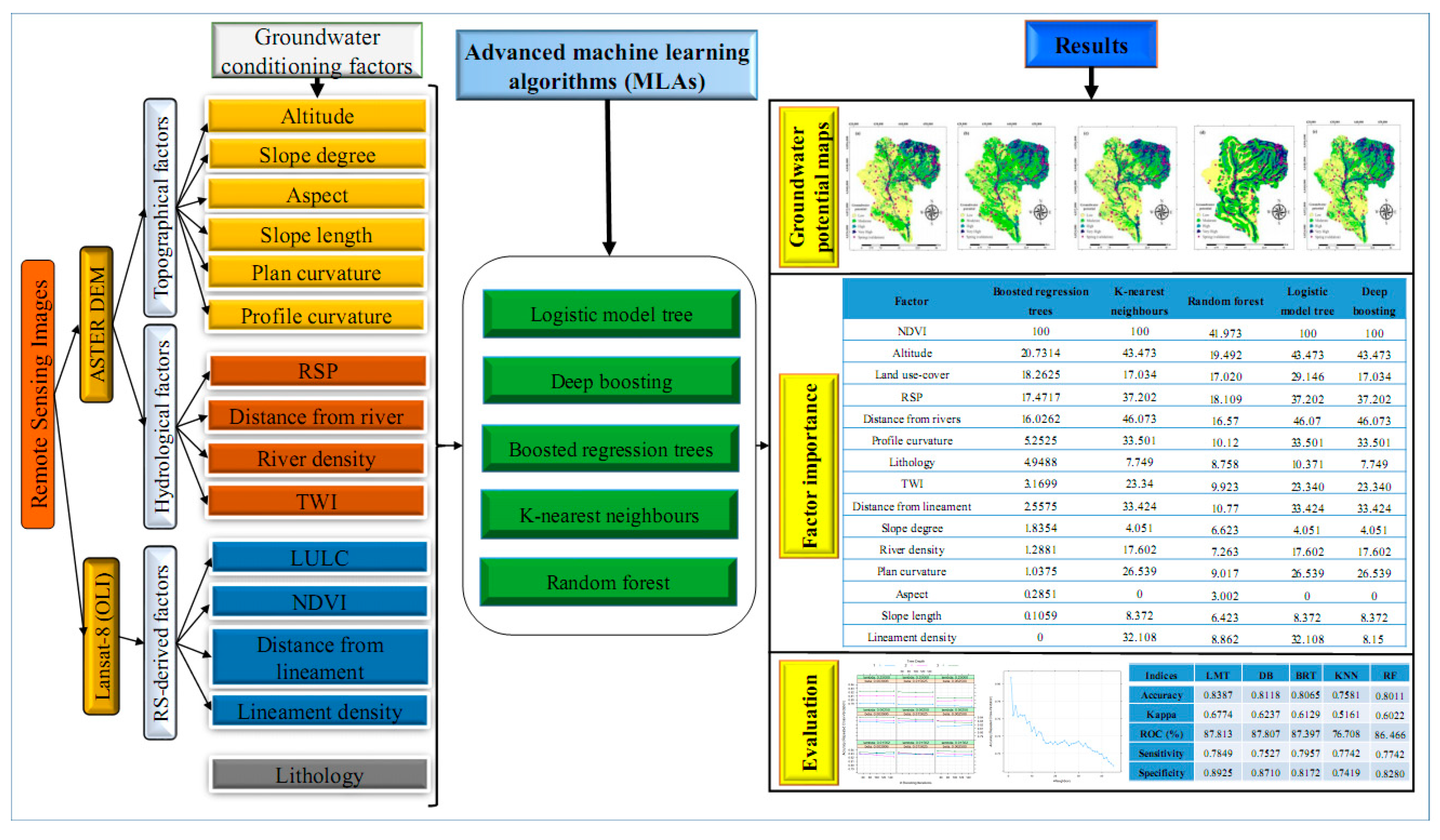
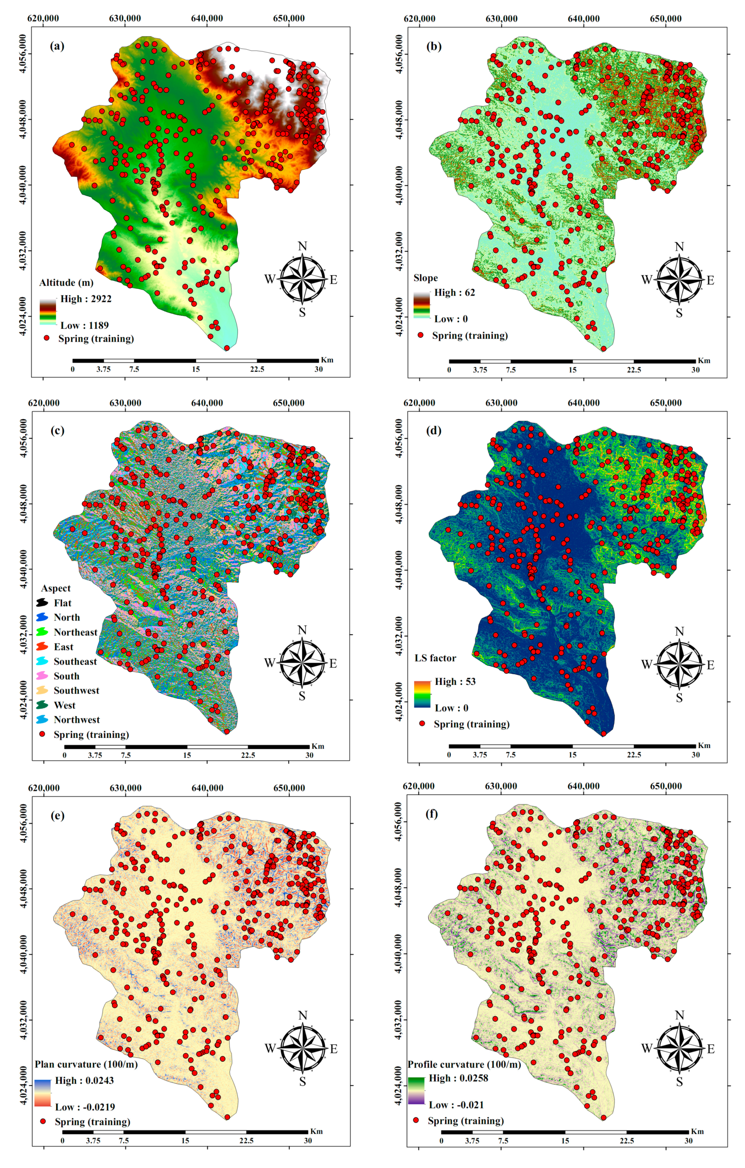
2.2. GW Spring Driving Factors

Generally, the productivity of GW for a given aquifer depends on a variety of components, such as topographical and hydrological, which rely on the accessibility and quality of data. In general, RS data are extensive with high resolution spatial information. To assemble topographical and hydrological variables, Advanced Spaceborne Thermal Emission and Reflection Radiometer (ASTER) Global Digital Elevation Model (GDEM) data, with a spatial resolution of 30 m, were acquired from the National Aeronautics and Space Administration (NASA) website. Next, topographical, and hydrological driving factors were computed using the DEM explained in the below sections.

2.2.1. Topographical Driving Factors

Altitude

Altitude has a vital implication on climate conditions and leads to a diverse categorization of vegetation and soil in any area [32,33]. Apart from this, it impacts GW potential indirectly; for instance, lower altitudes have lower slopes and the rate of infiltration enhances accordingly [34,35]. The altitude map of the Hesare-No basin was extracted from the “ASTER-DEM.” It varies between 1189 and 2922 m with a mean altitude of about 1691 m (Figure 3a).

Slope Degree

Slope degree was derived from the elevation variation and is looked upon as a primary component of the surface water flow regime due to the influence of gravity on water movement [36]. Runoff generation is directly proportional to the slope and GW recharge is greater in areas with lower slopes [37]. Water flow on gentle slopes is slow and the infiltration rate increases recharge to the aquifer, while steep slopes increase water flow velocity, hence the decreased recharge [38]. The slope map of the Hesare-No basin ranges between 0 and 62 degrees (Figure 3b).

Aspect

Aspect represents the dominant direction of the slope and indicates the direction of the drainage system [39]. Generally, aspect is used in hilly and mountainous regions, because sunshine or shadow duration plays a critical role in determination of the soil moisture [36]. The aspect also affects the amount of runoff generation through impacting vegetation growth and GW augmentation [40]. This factor is classified into nine categories as depicted in Figure 3c.

Slope Length (LS)

The LS factor is a combination of two components consisting of “slope length (L) and slope steepness (S)” that signifies the ratio of soil loss per unit basin area [7,41]. This factor can be calculated by [42]:

$$LS={\left(\frac{B_s}{22.13}\right)}^{0.6}{\left(\frac{\sin \alpha }{0.0896}\right)}^{1.3}$$

(1)

where B_s is the specific basin area (m²) and α is the slope gradient in degrees. The LS of the Hesare-No area ranges between 0 and 53 (m) (Figure 3d).

Plan and Profile Curvatures

The curvature displays the change of topography and consists of two major parts, i.e., “profile and plan curvature,” which affect the acceleration or deceleration and the convergence or divergence of the flow across the surface, respectively [43]. These driving factors were created using SAGA-GIS (SAGA User Group Association, Hamburg, Germany) (Figure 3f).

Relative Slope Position (RSP)

RSP can be used to distinguish between topographical properties, e.g., “ridge peaks, valleys, mid-slopes, flat surfaces, foot-slopes, and upper slopes” [8]. The RSP is one of the contributing variables for GW potential [44,45]. In this research, the RSP map was produced implementing SAGA-GIS (Figure 3g).

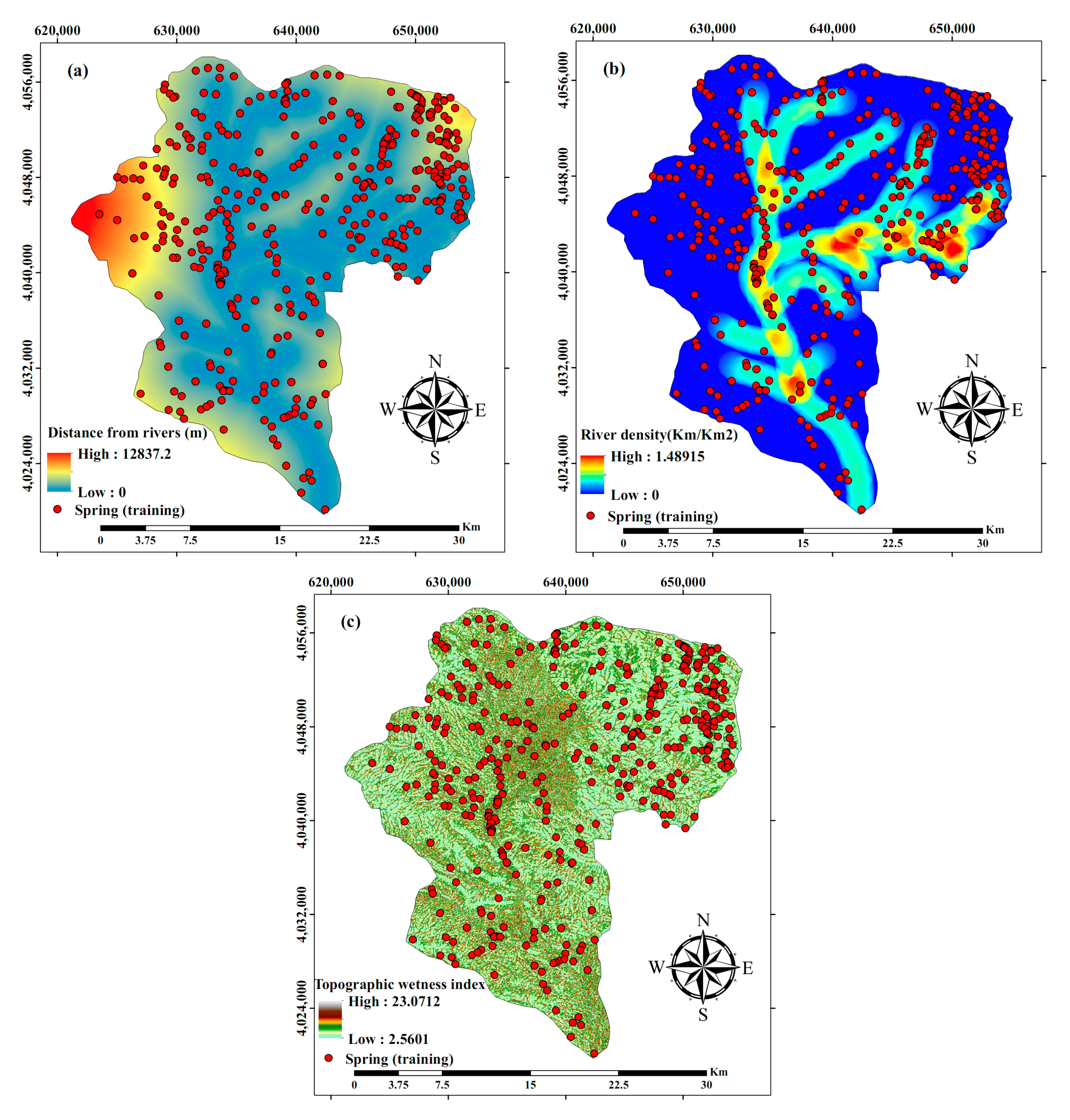
2.2.2. Hydrological Driving Factors

Distance from Rivers and River Density (Rd)

Rivers are the principal origin of GW recharge in semiarid regions. Hence, distance from rivers is one of the major hydrological elements affecting GW potential. This layer was generated in accordance with the “Euclidean distance function” (Figure 4a).

River density (Rd) is another hydrological driving factor that is explained by the ratio of the total length of the river system to the total area of any given pixel [46]. Rd depends on river location, runoff generation, vegetation cover, climate, and lithology [47]. Therefore, Rd fulfils a critical role in the appraisal of GW potential for any given watershed. Rd was calculated employing the line density function in ArcGIS. The Rd map of the area ranges between 0 and 1.5 km/km² (Figure 4b).

Topographic Wetness Index (TWI)

TWI is used to demonstrate the spatial pattern of moisture and delineate the impacts of topographic conditions for locating the size of runoff saturated areas [39,48]. It plays a major role in the transport and accumulation of runoff at the soil surface. Greater TWI values demonstrate better GW retention capability of an area [7]. The TWI factor is calculated as:

$$TWI=ln\left(\frac{\beta }{\tan \alpha }\right)$$

(2)

where β is the cumulative upslope area drained through a particular point (per unit contour length), and α is the gradient of the slope in that point. The TWI in the Hesare-No area varies between 2.5 and 23 (Figure 4c).

2.2.3. RS-Derived Factors

Satellite Data and Pre-Processing

To produce RS-derived factors such as LULC, NDVI, distance from lineament, and lineament density, Landsat-8 (OLI) data in 2019 (August), provided by the “United States Geological Survey (USGS),” were acquired. The image was clear and nearly “cloud-free” (with total cloud cover less than 1%). Pre-processing of the image comprised “radiometric calibration,” “QUick atmospheric correction,” and “geometric correction” algorithms using ENVI software. The pre-processing was conducted to convert the digital numbers of the multi-spectral bands (band 1–7) to “surface reflectance” (ranging from 0 to 1). To increase the resolution of the multi-spectral bands in the Landsat-8 image from 30 to 15 m, the “Gram–Schmidt method” was used for pan-sharpening in ENVI. This is a method to increase the lower spatial resolution of the multi-spectral Landsat images based on higher resolution of panchromatic imagery. Finally, the following factors were generated:

Generation of Land Use/Land-Cover Classification and Accuracy Assessment

Many studies have underlined the importance of LULC in the hydrological interpretation for the development of GW potential [44,49,50]. The presence and productivity of GW in a particular area as well relies upon the soil surface features, which act as a mediator in the process of “runoff-infiltration and runoff-evapotranspiration” [51]. Hence, to detect LULC variation for the Hesare-No Basin, multi-spectral bands of Landsat-8 (OLI) images and three supervised classification algorithms, i.e., maximum likelihood, neural network, and decision tree, were implemented. The Hesare-No Basin was categorized into five principal LULCs encompassing “orchard, agriculture, bare land, rangeland, and water surface.” Validation of the LULC maps was conducted by electing 50 checkpoints (through random sampling) on the ground for each LULC class compared with the corresponding grid in the satellite images by calculating the overall accuracy and kappa coefficients. These indices are frequently used as quantitative validation indices [52,53]. The validation results are depicted in

Table 1. Accuracy assessment of land use/cover (LULC) classification for the Hesare-No Basin.

Indices	Classification Algorithm
	Maximum Likelihood	Neural Network	Decision Tree
Overall Accuracy (%)	87	88	91
Kappa Coefficient (%)	76	78	82

. The table shows that the overall accuracy for the maximum likelihood, neural network, and decision tree algorithms was 87%, 88%, and 91%, respectively, while the kappa coefficients were 76%, 78%, and 82%, respectively. According to previous research, kappa coefficients greater than 75% demonstrate that the classification and ground truth data are comparable [54]. Thus, the decision tree algorithm was implemented to create the LULC map for the Hesare-No Basin due to its greater efficiency (Figure 5a). The LULC map demonstrated that 0.03%, 1%, 11.5%, 37.8%, and 49.7% of the Hesare-No Basin are covered by water surface, orchards, agriculture, bare land, and rangeland, respectively.

Retrieval of Normalized Difference Vegetation Index (NDVI)

NDVI is one of the primary indicators to measure vegetation cover. NDVI values between 0.1 and 0.75, in general, denote vegetation cover, while values greater than 0.75 imply a dense canopy. The NDVI for bare land and soil is close to zero, and negative values indicate water surface such as reservoirs [55]. The NDVI was calculated from the red and near infrared bands using:

$$\mathrm{NDVI}=\left(\frac{\mathrm{NIR}-\mathrm{Red}}{\mathrm{NIR}+\mathrm{Red}}\right)$$

(3)

where NIR refers to surface reflectance of band 5 (Landsat-8), and Red refers to surface reflectance of band 4 (Landsat-8). The distribution map of NDVI is shown in Figure 5b.

Distance from Lineament and Lineament Density

The distance from lineaments is beneficial for GW potential assessment as the target hydrogeological zones that are located adjacent to linear structures control the movement and storage of GW [13,56]. It also describes surface morphologies such as “faults, fractures, cracks,” as well as provides information on the infiltration of water depending on rock properties [51]. The distance from lineaments in the Hesare-No Basin was provisioned from the Landsat-8 OLI image as shown in Figure 5c. Another factor is lineament density, which is utilized to distinguish areas with great lineament concentrations that are correlated with permeability and GW potential [57]. Lineament density illustrates the total length of lineaments in a unit area, which is calculated by a line density function. The distribution map of the lineament density factor is shown in Figure 5d.

2.2.4. Lithology

Geological formations are important for GW potential, influencing the porosity and permeability of the aquifer material [12,58]. The geology controls the quantity and quality of GW [13]. The geological map was obtained from the Iranian Department of Geological Survey [59]. Accordingly, the Hesare-No Basin was grouped into 15 lithological units with differences in both lithology and geological age (

Table 2. Types of lithological formation in the Hesare-No Basin.

Geology Group	Description	Age
Jmz	Grey thick-bedded limestone and dolomite (Mozduran formation)	Middle-Late Jurassic
Jd	Well-bedded to thin-bedded, greenish-grey argillaceous limestone with intercalations of calcareous shale (Dalichai formation)	Jurassic
PlQc	Fluvial conglomerate, Piedmont conglomerate, and sandstone	Pliocene-Quaternary
Jl	Light grey, thin-bedded to massive limestone (Lar formation)	Jurassic-Cretaceous
Qft2	Low level piedmont fan and valley terrace deposits	Quaternary
Ea.bvt	Andesitic to basaltic volcanic tuff	Eocene
PlQdv	Rhyolitic to Rhyodacitic volcanics	Pliocene-Quaternary
Jph	Phyllite, slate, and meta-sandstone (Hamadan Phyllites)	Jurassic
E3c	Conglomerate and sandstone	Eocene
E2sht	Tuffaceous shale and tuff	Eocene
E2m	Pale red marl, gypsiferous marl, and limestone	Eocene
Mur	Red marl, gypsiferous marl, sandstone, and conglomerate (Upper Red formation)	Miocene
Pz	Undifferentiated lower Paleozoic rocks	Early Palaeozoic
Osh	Greenish-grey siltstone and shale with intercalations of flaggy limestone (Shirgesht formation)	Ordovician
Eav	Andesitic volcanics	Middle Eocene

, Figure 6).

2.3. Machine Learning Algorithms

2.3.1. Logistic Model Tree

Logistic model tree is a classification MLA that integrates the “C4.5 and LR algorithms” [60]. These include a tree structure with a number of inner nodes and leaves [61]. The “information gain” is utilized to divide, and the LogitBoost is employed to build a LR at each node [62]. The logistic model tree implements the CART to prune the trees [63], and implements cross-validation for exploring the number of iterations of logitBoost to tackle overfitting [26]. Logistic model tree employs the C4.5 at nodes and LR to explore the probability within a leaf node as:

$$P\left(N|x\right)=\raisebox{1ex}{$\exp \left(L_i\left(x\right)\right)$}\!\left/ \!\raisebox{-1ex}{${{\displaystyle \sum }}_{i=1}^n\exp \left(L_i\left(x\right)\right)$}\right.$$

(4)

where $P\left(N|x\right)$ presents “posterior probability” in a leaf node of N categories within the input vector x, and $L_i\left(x\right)$ denotes the least square fits obtained as:

$$L_i\left(x\right)={\displaystyle \sum }_{i=1}^n{\mathsf{\alpha }}_i{\mathrm{x}}_i+{\mathsf{\alpha }}_0=0$$

(5)

where n is the number of driving factors, and ${\mathsf{\alpha }}_0$ and ${\mathsf{\alpha }}_i$ are the coefficients of the component of vector x = x_i, representing the driving factors. To apply the logistic model tree, R statistical software (R Foundation for Statistical Computing, Vienna, Austria) and two packages including “caret” [64] and “RWeka” [65] were used through a 10-fold cross-validation.

2.3.2. Deep Boosting

Deep boosting was introduced by Cortes et al. [28] and implements a number of deep decision trees to obtain highly accurate outputs. The major feature of this method is a “capacity-conscious element” for hypothesis choice [28]. The method is a boosting-based MLAs and an ensemble of many weak learners in order to obtain a high accuracy output. A full description of the deep boosting can be found in Cortes et al. [28]. To run the deep boosting algorithm, “caret” [64] and “deepboost” [66] packages were run in R statistical software considering a 10-fold cross-validation.

2.3.3. Boosted Regression Trees

Boosted regression trees are one of many ensemble MLAs that enhance the efficacy as well as prediction capability of single methods by making use of many trees [7,41,67,68]. Two influential components, namely “gradient boosting” and “classification and regression tree,” are integrated in boosted regression trees [69]. Boosting is applied to enhance the predictive accuracy of regression trees, and is related to the CART class of algorithms [41]. Decision trees display information from great data amounts in an efficient manner that is straightforward, comprehensible, and quick. It is less susceptible to over-fitting [67,70]. In boosted regression trees, three factors are required to be optimized, i.e., “number of trees,” “interaction depth,” and “shrinkage” [69]. The boosted regression trees can be calculated based on previous literature [41,68,71]. To run the boosted regression trees algorithm, caret [64] and gbm [72] packages were conducted in the R statistical software through a 10-fold cross-validation scheme.

2.3.4. K-Nearest Neighbors

The k-nearest neighbors technique is a common classification MLA that is nonparametric and eliminates estimation of the class density function [73]. This algorithm has been implemented in processes such as GW, landslide, gully erosion, and flood mapping [17,74,75]. The main assumption of the k-nearest neighbors is that unknown cells are classified based on their similarity to cells in the training set [76], which is explained through the Euclidean distance application [77]. To exemplify the classification procedure in the k-nearest neighbors, an illustrative case is presented in Figure 7. The blue triangle in the figure is an unknown cell, and the target is to distinguish whether it is a GW spring or not. If the value of K (number of nearest neighbors) is equal to 3 (the internal dashed circle), it will be assumed to be a spring (green squares) since there are two springs and one non-spring (red circle) in the inward dashed circle. However, if the value of k is equal to 9 (the external dashed circle), it would be interpreted as a non-GW spring, as there are five non-spring cells and four springs in the outer dashed circle. To run k-nearest neighbors in this study, the caret package [64] was applied in the R statistical software through a 10-fold cross-validation scheme.

2.3.5. Random Forest

Random forest is another vigorous and efficient MLA that was developed by Breiman [78] as an extension of the “classification and regression trees” to promote its prediction competence [39]. Numerous decision trees are fabricated through randomly bootstrapped calibration sets [78]. Afterwards, the model integrates the average outcomes of all the trees [8]. The user shall select two parameters, i.e., “the number of variables at each split” and “the number of tree” [39]. This model does not use all available data to grow the tree; it utilizes 66.66% of the Bootstrap information. Then, 33.33% of the remaining data are used to evaluate the fitted tree. In this research, this model was applied through the ‘randomForest’ package [79] in the R statistical software.

2.4. Validation of the Algorithms

The performance of the logistic model tree, deep boosting, boosted regression trees, and k-nearest neighbors in the investigation of GW potential was assessed by utilizing the receiver operating characteristic (ROC) curve, accuracy, kappa, sensitivity, and specificity [8,12,80,81,82]. To quantify the prediction accuracy, the area under the ROC curve (AUC) was computed. The AUC values from 0.7 to 0.8 indicate that the prediction accuracy is acceptable, AUC ranging from 0.8 to 0.9 indicates excellent, and greater than 0.9 shows outstanding results [44].

Sensitivity and specificity indicators are the percentage of correctly classified pixels in regions with high and low GW potential, respectively. Sensitivity and specificity are calculated as:

$$Sensitivity=\frac{TP}{TP+FN}$$

(6)

$$Specificity=\frac{TN}{FP+TN}$$

(7)

where TP is “true positives,” FN is “false negatives,” TN is “true negatives,” and FP is “false positives.” TP and TN are the number of pixels that are correctly classified, whereas FP and FN are the number of pixels erroneously classified. Accuracy and kappa indicators are calculated as:

$$Accuracy=\frac{TP+NT}{TP+NT+FP+FN},$$

(8)

$$Kappa=\frac{P_{obs}-P_{exp}}{1-P_{obs}},$$

(9)

$$P_{obs}=TP-\frac{TN}{n},$$

(10)

$$P_{exp}=\left(TP+FN\right)\left(TP+FP\right)+\left(FP+TN\right)\frac{\left(FN+TN\right)}{\sqrt{N}},$$

(11)

where n is the proportion of pixels that are properly categorized as spring or non-spring, and N is the total number of training pixels. Kappa ranges between 0 and 1, and the closer to 1 indicates a better accuracy. At last, for determining the significant difference of the algorithms’ outputs, we implemented the Friedman test. The Friedman test is a “non-parametric” test equivalent to the repeated measures analysis of variance (ANOVA). Under the null-hypothesis, it depicts that all the algorithms are equivalent, so a rejection of this hypothesis shows the existence of differences among the efficiency of all the algorithms investigated. To do so, all the computed accuracy indices for the algorithms were considered. It is noteworthy to mention that area under the ROC curve was considered between 0 and 1 like other indices.

3. Results

3.1. Machine Learning Algorithm Parameter Optimization Results

All MLAs were optimized based upon a 10-fold cross-validation. The logistic model tree was constructed by 21 “iterations,” leading to accuracy and kappa values of 0.83, and 0.66, respectively. As per the deep boosting algorithm, the final parameter optimization is presented in Figure 8. As observed, deep boosting was constructed with 100 iterations, “tree depth” equal to 3, beta equal to 0.0039, lambda equal to 0.0625, and “loss type” equal to l with accuracy and kappa values of 0.840, and 0.681, respectively. In the k-nearest neighbors algorithm, a k value equal to 1 among values from 1 to 45 was opted as the best parameter (Figure 8). Further, a significantly diminishing trend was observed between the accuracy of the k-nearest neighbors and the k. The calculated accuracy and kappa indices for the k-nearest neighbors were 0.807 and 0.614, respectively. In the case of the boosted regression trees algorithm, it was optimized with 200 trees, “interaction depth” of 3, shrinkage of 0.01, and “minimum terminal node” size of 20, leading to accuracy and kappa values of 0.840 and 0.680, respectively. The results of the random forest algorithm showed that it was tuned with “Minimum size of terminal nodes” of five, three variables at each node, and 700 trees.

3.2. Validation of Maps and Performance Analysis of the Algorithms

The validation outcomes for the MLAs in this research are illustrated in

Table 3. Evaluation of the advanced machine learning algorithms (MLAs) with different indices.

Indices	Logistic Model Tree	Deep Boosting	Boosted Regression Trees	K-Nearest Neighbors	Random Forest
Accuracy	0.8387	0.8118	0.8065	0.7581	0.8010
Kappa	0.6774	0.6237	0.6129	0.5161	0.6022
ROC (%)	87.813	87.807	87.397	76.708	86.466
Sensitivity	0.7849	0.7527	0.7957	0.7742	0.7750
Specificity	0.8925	0.8710	0.8172	0.7419	0.8270

. Based on the table, deep boosting and logistic model tree algorithms had slightly better performances than the boosted regression trees and random forest algorithm, and much higher performances than the k-nearest neighbors algorithm regarding accuracy, kappa, and ROC. In a more detailed view, regarding specificity, it is seen that the logistic model tree and deep boosting algorithms had the highest ability to predict the field data, while the boosted regression trees algorithm showed a slightly higher performance in determining absence points.

The non-parametric Friedman test with a p-value threshold of 0.05 was performed to compare the performances of MLAs. The findings of the five groundwater potential models from the Friedman test are shown in

Table 4. Comparison of the five MLAs using the Friedman test.

Mean Rank					p-Value (α = 0.05)	χ2 (Chi-Square)
Logistic Model Tree	Deep Boosting	Boosted Regression Trees	K-Nearest Neighbors	Random Forest
4.80	3.40	3.20	1.20	2.40	0.007	14.08

. The findings indicate that the p-values were lower than 0.05 (0.007); thus, the null hypothesis is rejected, which indicates the existence of statistically significant differences between the performances of the models.

3.3. GW Potential Maps

The results of the GW potential maps produced by the logistic model tree, deep boosting, boosted regression trees, k-nearest neighbors, and random forest are depicted in Figure 9. In line with previous research [9,13,39,83], the natural break (Jenks) method was utilized to classify the GW potential maps into four classes of “low, moderate, high, and very high.” The MLAs illustrated a similar pattern of GW potential in the Hesare-No Basin. However, for GW exploitation, the GW potential map generated by the logistic model tree is suggested regarding its superior performance. This map implies that the closest areas, as well as areas along the rivers, are assigned as very high GW potential (Figure 9). The north-eastern part of the study region has higher GW potential and is recommended for GW exploitation. On the other hand, the map reveals that the eastern part of the Hesare-No Basin is categorized as low GW potential, which can be associated with greater distances to rivers. This information can be used for water resources and also land use management. The calculated range and total area of each class are presented in

Table 5. Range and area of each class of the GW potential maps constructed by the logistic model tree, deep boosting, boosted regression trees, and k-nearest neighbors.

Model/Class		Low	Moderate	High	Very High
Logistic model tree	Range	0–0.11	0.11–0.37	0.37–0.70	0.70–1
	Area (km2)	371.02	169	79.22	92.9
Deep boosting	Range	0.02–0.27	0.27–0.43	0.43–0.60	0.60–0.98
	Area (km2)	230.23	277.32	141.73	62.83
Boosted regression trees	Range	0.09–0.21	0.21–0.39	0.39–0.62	0.62–0.89
	Area (km2)	342.25	172.48	109.87	87.44
K-nearest neighbors	Range	0–0.04	0.04–0.42	0.42–0.71	0.71–1
	Area (km2)	220.9	280.68	99.8	110.77
Random forest	Range	0–0.16	0.16–0.36	0.36–0.61	0.61–1
	Area (km2)	315.06	198.71	124.42	73.93

. The results reveal that 110.77, 92.90, 78.44, 73.93, and 62.83 km² of the Hesare-No Basin are classified as very high GW potential by the k-nearest neighbors, logistic model tree, boosted regression trees, random forest, and deep boosting, respectively. On the other hand, low GW potential was predicted to cover 371.02, 342.25, 315.04, 230.23, and 220.90 km² of the total basin area by the logistic model tree, boosted regression trees, random forest, deep boosting, and k-nearest neighbors, respectively. The percentage of each class by the logistic model tree, deep boosting, boosted regression trees, k-nearest neighbors, and random forest is shown in Figure 10. It can be observed that 29%, 28%, 27%, 27%, and 24% of the Hesare-No Basin are classified as high and very high GW potential by the k-nearest neighbors, deep boosting, random forest, boosted regression trees, and logistic model tree, respectively. Additionally, it was demonstrated that the highest percentage of “low, moderate, high, and very high” classes belonged to the logistic model tree, k-nearest neighbors, deep boosting, and k-nearest neighbors MLAs, respectively.

3.4. Importance of Factors

Table 6. Importance of driving factors in GW potential assessment.

Factor	Boosted Regression Trees (Relative Influence)	K-Nearest Neighbors	Random Forest(Mean Decrease Gini)	Logistic Model Tree
NDVI	100	100	41.973	100
Distance from rivers	16.03	46.073	16.57	46.07
Altitude	20.73	43.473	19.492	43.473
RSP	17.47	37.202	18.109	37.202
Profile curvature	5.25	33.501	10.12	33.501
Distance from lineament	2.558	33.424	10.77	33.424
Lineament density	0	32.108	8.862	32.108
Land use-cover	18.26	17.034	17.02	29.146
Plan curvature	1.038	26.539	9.017	26.539
TWI	3.17	23.34	9.923	23.34
River density	1.288	17.602	7.263	17.602
Lithology	4.949	7.749	8.758	10.371
Slope length	0.105	8.372	6.423	8.372
Slope degree	1.835	4.051	6.623	4.051
Aspect	0.285	0	3.002	0

NDVI––normalized difference vegetation index, RSP––Relative Slope Position, TWI––Topographic Wetness Index

presents the importance of the driving factors in the modelling procedure for the Hesare-No Basin obtained by different MLAs. The importance of the driving factors is sorted based on logistic model tree results. It should be noted that the logistic model tree obtained the highest accuracy. As can be seen, the NDVI was found to be the most important factor in the modelling with all assessed MLAs. The secondary important factor was distance from the rivers in the logistic model tree, while altitude was the second important factor in boosted regression trees and random forest with 20.73 and 19.46 values, respectively. Moreover, the results indicate that altitude generally is the third important factor. Overall, RSP and LULC, with significant differences, are specified as the other important factors. The results also illustrate that distance from lineament and lineament density factors could be contributed moderately to the groundwater potential mapping. However, aspect, slope degree, and slope length factors had the lowest important value in all MLAs, generally.

4. Discussion

Pinpointing areas with high GW potential based on spring data is regarded as a significant method for the proper conservation and management of freshwater supplies, in particular in semi-arid districts. Hence, MLAs and RS-derived driving factors have been gaining popularity in this field. To qualitatively assess the outcomes, logistic model tree, boosted regression trees, deep boosting, and random forest algorithms led to GW potential maps with AUC values between 0.8 and 0.9, categorizing them as “very good” predictors, while k-nearest neighbors had an AUC value between 0.7 and 0.8, categorizing it as a “good” predictor based on Yesilnacar and Topal [84]. More precisely, the outputs reveal that the deep boosting and logistics model tree produced competitive and slightly better performances than the boosted regression tree algorithm. The deep boosting and logistic model tree also had better performances than the random forest with area under the ROC curve differences of greater than 1.4%. This difference proves their acceptable performance based on this fact that random forest has been reported as a strong algorithm in groundwater potential mapping [8,16]. Based on Friedman non-parametric test results, the difference in the performance of the algorithms is statistically significant. The logistic model tree and deep boosting algorithms have the potential to be strengthened by using parameter optimization algorithms, such as the genetic algorithm, to improve their accuracy [85]. As an example of the impact of the genetic algorithm on groundwater potential algorithms, we can refer to Naghibi et al. [85], which used the genetic algorithm to optimize random forest and confirmed its considerable impact on the model’s performance.

The greater accuracy of the logistic model tree could be associated with the fact that it benefits from the CART algorithm, which assists pruning of the trees and hinders them from “overfitting.” The stated feature of the logistic model tree accompanied by the application of LogitBoost can be the reason for its superior performance [86]. Similarly, high accuracy of the logistic model tree is declared by researchers in spatial investigations such as flash flood susceptibility, landslides, and gully erosion [29,31,87]. Deep boosting takes advantage of the data analyses and the favorable learning ability [28], which are the reasons for its superior performance in generating a GW potential map. On the other hand, boosted regression trees also produced high accuracy maps, which could be due to the fact that they keep important GW conditioning factors, detect the interactions, model distinct kinds of factors, and finally, manage missing data [17,88]. Their acceptable efficiency is in line with the previous studies [7,17,69]. Further, the great accuracy of the random forest model could be due to its low aptitude to overfitting, and the capability to support high-dimensional datasets [17,89]. For weaker performance of the k-nearest neighbors algorithm, this can be referred to its sensitivity to unrelated and unnecessary data as all characteristics are involved in the similarity and have a role in the final prediction.

Among the seven highly important driving factors, three, i.e., NDVI, distance from lineament, and lineament density, are direct RS-derived products. Except the RS-based factors, distance from rivers, altitude, RSP, and profile curvature are other important factors in the assessment of GW potential in the study region. This fact highlights the great impact of the RS-derived data on GW studies and necessitates the demand for high-accuracy RS products in future research on GW potential. The NDVI was ranked as the most influencing factor since it represents the vegetation cover and impacts the velocity of “water flow” and, therefore, “soil infiltration rate.” The results are in agreement with Davoodi-Moghaddam et al. [8] and Naghibi et al. [17], which indicated that the NDVI factor is the most significant factor for groundwater potential mapping. Furthermore, the great influence of distance from rivers can be associated with the impact of rivers on GW natural recharge. As stated, rivers are the primary sources of natural GW augmentation particularly in arid and semiarid regions [90]. Moreover, the large contribution of the altitude, RSP, and profile curvature can be connected to the influence of topography on drainage system development, water movement, and subsequently, the soil infiltration rate. With respect to lineament-based factors, their greater influence could be linked to their controlling role in soil infiltration, and the GW movement and storage in an aquifer. Several studies have shown that NDVI [20], distance from rivers [9] altitude [6,41], and RSP [7,44] are highly contributing factors to assess GW potential, which is in line with our outcomes.

5. Conclusions

Accurate appraisal of GW supplies is fundamental in reaching sustainable development. However, there is often a general shortage of detailed hydro-geological data of aquifers and their productivity in developing countries. RS-based data products can offer a wealth of information for the data-scarce regions. This study applied the two new algorithms, deep boosting and logistic model tree, and compared them with the three benchmarks, i.e., boosted regression trees, k-nearest neighbors, and random forest MLAs. The outcome was satisfying in accordance with the AUC and accuracy scores. The deep boosting and logistic model tree models produced accurate and similar maps compared to the boosted regression trees, and outperformed the random forest and k-nearest neighbors algorithm. This emphasizes that the new MLAs, i.e., deep boosting and logistic model tree, can be used in GW studies to detect areas with high potential for GW exploitation. The other target of the current research was to scrutinize the importance of the factors in GW potential assessment, which demonstrated that the NDVI with high difference was the most important factor, followed by the distance from rivers, altitude, RSP, profile curvature, distance from lineaments, and lineaments density. This highlights the outstanding contribution of the NDVI factor and the considerable impact of lineament-based factors among the impact of DEM-derived factors. This approves the high influence of RS-derived factors on the modelling process. Using RS-based data is indeed a potential alternative for areas confronted with lack of data, and in particular, hydrogeological information, which is difficult to access. Overall, a combination of RS and DEM-derived data can provide sufficient amount of relationships for GW studies. As per transferability, in the case of the algorithms, all of them are freely available in the R statistical software and can be used by the water resources managers. Moreover, this study used the ASTER digital elevation model, which is freely available. Further, RS-derived factors were obtained by Landsat-8 (OLI) images that are also freely available worldwide. However, two other factors, including spring locations and lithology, might not be available in some areas, which can limit the application of the current methodology. In the case of springs as an indicator of GW potential, it can be replaced by the well discharge data. In the case of inaccessibility to both spring and well locations, researchers can utilize expert judgement-based approaches, such as the analytical hierarchy process, and define the weights of the factors and obtain GW potential maps. In the respect of lithology, it can be replaced by some other factors such as DEM-derived and other RS-based factors to feed the models with as much information and patterns as possible. Due to these limitations, we can recommend the application of the current methodology with some changes regarding the factors in other regions to tackle data insufficiency.

References

1. Wada, Y.; Van Beek, L.P.H.; Van Kempen, C.M.; Reckman, J.W.T.M.; Vasak, S.; Bierkens, M.F.P. Global depletion of groundwater resources. Geophys. Res. Lett. 2010, 37. [Google Scholar] [CrossRef] [Green Version]
2. Alcamo, J.; Henrich, T.; Rosch, T. World Water in 2025—Global Modelling and Scenario Analysis for the World Commission on Water for the 21st Century; Report A0002; Centre for Environmental System Research, University of Kassel: Kassel, Germany, 2000. [Google Scholar]
3. Chezgi, J.; Pourghasemi, H.R.; Naghibi, S.A.; Moradi, H.R.; Kheirkhah Zarkesh, M. Assessment of a spatial multi-criteria evaluation to site selection underground dams in the Alborz Province, Iran. Geocarto Int. 2016, 31, 628–646. [Google Scholar] [CrossRef]
4. Sahoo, S.; Munusamy, S.B.; Dhar, A.; Kar, A.; Ram, P. Appraising the accuracy of multi-class frequency ratio and weights of evidence method for delineation of regional groundwater potential zones in canal command system. Water Resour. Manag. 2017, 31, 4399–4413. [Google Scholar] [CrossRef]
5. Naghibi, S.A.; Pourghasemi, H.R.; Abbaspour, K. A comparison between ten advanced and soft computing models for groundwater qanat potential assessment in Iran using R and GIS. Theor. Appl. Climatol. 2018, 131, 967–984. [Google Scholar] [CrossRef]
6. Naghibi, S.A.; Moradi Dashtpagerdi, M. Evaluation of four supervised learning methods for groundwater spring potential mapping in Khalkhal region (Iran) using GIS-based features. Hydrogeol. J. 2017, 25, 169–189. [Google Scholar] [CrossRef]
7. Kim, J.C.; Jung, H.S.; Lee, S. Spatial mapping of the groundwater potential of the Geum River basin using ensemble models based on remote sensing images. Remote Sens. 2019, 11, 2285. [Google Scholar] [CrossRef] [Green Version]
8. Moghaddam, D.D.; Rahmati, O.; Haghizadeh, A.; Kalantari, Z. A modeling comparison of groundwater potential mapping in a mountain bedrock aquifer: QUEST, GARP, and RF models. Water 2020, 12, 679. [Google Scholar] [CrossRef] [Green Version]
9. Kalantar, B.; Al-Najjar, H.A.H.; Pradhan, B.; Saeidi, V.; Halin, A.A.; Ueda, N.; Naghibi, S.A. Optimized conditioning factors using machine learning techniques for groundwater potential mapping. Water 2019, 11, 1909. [Google Scholar] [CrossRef] [Green Version]
10. Naghibi, S.A.; Hashemi, H.; Berndtsson, R.; Lee, S. Application of extreme gradient boosting and parallel random forest algorithms for assessing groundwater spring potential using DEM-derived factors. J. Hydrol. 2020, 589, 125197. [Google Scholar] [CrossRef]
11. Corsini, A.; Cervi, F.; Ronchetti, F. Weight of evidence and artificial neural networks for potential groundwater spring mapping: An application to the Mt. Modino area (Northern Apennines, Italy). Geomorphology 2009, 111, 79–87. [Google Scholar] [CrossRef]
12. Lee, S.; Hyun, Y.; Lee, S.; Lee, M.-J. Groundwater potential mapping using remote sensing and GIS-based machine learning techniques. Remote Sens. 2020, 12, 1200. [Google Scholar] [CrossRef] [Green Version]
13. Al-Djazouli, M.O.; Elmorabiti, K.; Rahimi, A.; Amellah, O.; Fadil, O.A.M. Delineating of groundwater potential zones based on remote sensing, GIS and analytical hierarchical process: A case of Waddai, eastern Chad. GeoJournal 2020, 1–14. [Google Scholar] [CrossRef]
14. Martínez-Santos, P.; Renard, P. Mapping groundwater potential through an ensemble of big data methods. Groundwater 2020, 58, 583–597. [Google Scholar] [CrossRef] [PubMed]
15. Chen, W.; Panahi, M.; Khosravi, K.; Pourghasemi, H.R.; Rezaie, F.; Parvinnezhad, D. Spatial prediction of groundwater potentiality using ANFIS ensembled with teaching-learning-based and biogeography-based optimization. J. Hydrol. 2019, 572, 435–448. [Google Scholar] [CrossRef]
16. Moghaddam, D.D.; Rahmati, O.; Panahi, M.; Tiefenbacher, J.; Darabi, H.; Haghizadeh, A.; Haghighi, A.T.; Nalivan, O.A.; Tien Bui, D. The effect of sample size on different machine learning models for groundwater potential mapping in mountain bedrock aquifers. CATENA 2020, 187, 104421. [Google Scholar] [CrossRef]
17. Naghibi, S.A.; Dolatkordestani, M.; Rezaei, A.; Amouzegari, P.; Heravi, M.T.; Kalantar, B.; Pradhan, B. Application of rotation forest with decision trees as base classifier and a novel ensemble model in spatial modeling of groundwater potential. Environ. Monit. Assess. 2019, 191, 1–20. [Google Scholar] [CrossRef]
18. Ozdemir, A. Using a binary logistic regression method and GIS for evaluating and mapping the groundwater spring potential in the Sultan Mountains (Aksehir, Turkey). J. Hydrol. 2011, 405, 123–136. [Google Scholar] [CrossRef]
19. Ozdemir, A. GIS-based groundwater spring potential mapping in the Sultan Mountains (Konya, Turkey) using frequency ratio, weights of evidence and logistic regression methods and their comparison. J. Hydrol. 2011, 411, 290–308. [Google Scholar] [CrossRef]
20. Naghibi, S.A.; Moghaddam, D.D.; Kalantar, B.; Pradhan, B.; Kisi, O. A comparative assessment of GIS-based data mining models and a novel ensemble model in groundwater well potential mapping. J. Hydrol. 2017, 548, 471–483. [Google Scholar] [CrossRef]
21. Nguyen, P.T.; Ha, D.H.; Avand, M.; Jaafari, A.; Nguyen, H.D.; Al-Ansari, N.; Van Phong, T.; Sharma, R.; Kumar, R.; Van Le, H.; et al. Soft computing ensemble models based on logistic regression for groundwater potential mapping. Appl. Sci. 2020, 10, 2469. [Google Scholar] [CrossRef] [Green Version]
22. Chen, W.; Li, H.; Hou, E.; Wang, S.; Wang, G.; Panahi, M.; Li, T.; Peng, T.; Guo, C.; Niu, C.; et al. GIS-based groundwater potential analysis using novel ensemble weights-of-evidence with logistic regression and functional tree models. Sci. Total Environ. 2018, 634, 853–867. [Google Scholar] [CrossRef] [PubMed] [Green Version]
23. Kim, J.C.; Jung, H.S.; Lee, S. Groundwater productivity potential mapping using frequency ratio and evidential belief function and artificial neural network models: Focus on topographic factors. J. Hydroinformatics 2018, 20, 1436–1451. [Google Scholar] [CrossRef]
24. Chapi, K.; Singh, V.P.; Shirzadi, A.; Shahabi, H.; Bui, D.T.; Pham, B.T.; Khosravi, K. A novel hybrid artificial intelligence approach for flood susceptibility assessment. Environ. Model. Softw. 2017, 95, 229–245. [Google Scholar] [CrossRef]
25. Tien Bui, D.; Bui, Q.T.; Nguyen, Q.P.; Pradhan, B.; Nampak, H.; Trinh, P.T. A hybrid artificial intelligence approach using GIS-based neural-fuzzy inference system and particle swarm optimization for forest fire susceptibility modeling at a tropical area. Agric. For. Meteorol. 2017, 233, 32–44. [Google Scholar] [CrossRef]
26. Chen, W.; Xie, X.; Wang, J.; Pradhan, B.; Hong, H.; Bui, D.T.; Duan, Z.; Ma, J. A comparative study of logistic model tree, random forest, and classification and regression tree models for spatial prediction of landslide susceptibility. CATENA 2017, 151, 147–160. [Google Scholar] [CrossRef] [Green Version]
27. Colkesen, I.; Kavzoglu, T. The use of logistic model tree (LMT) for pixel and object based classifications using high resolution WorldView 2 imagery. Geocarto Int. 2017, 32, 71–86. [Google Scholar] [CrossRef]
28. Cortes, C.; Mohri, M.; Syed, U. Deep Boosting. In Proceedings of the 31st International Conference on International Conference on Machine Learning, Beijing, China, 21–26 June 2014; Volume 32, pp. 1179–1187. [Google Scholar]
29. Pham, B.T.; Van Phong, T.; Nguyen, H.D.; Qi, C.; Al-Ansari, N.; Amini, A.; Ho, L.S.; Tuyen, T.T.; Yen, H.P.H.; Ly, H.-B.; et al. A comparative study of kernel logistic regression, radial basis function classifier, multinomial naïve bayes, and logistic model tree for flash flood susceptibility mapping. Water 2020, 12, 239. [Google Scholar] [CrossRef] [Green Version]
30. Khosravi, K.; Melesse, A.M.; Shahabi, H.; Shirzadi, A.; Chapi, K.; Hong, H. Flood susceptibility mapping at Ningdu catchment, China using bivariate and data mining techniques. In Extreme Hydrology and Climate Variability; Elsevier: Amsterdam, The Netherlands, 2019; pp. 419–434. [Google Scholar]
31. Nhu, V.-H.; Shirzadi, A.; Shahabi, H.; Singh, S.K.; Al-Ansari, N.; Clague, J.J.; Jaafari, A.; Chen, W.; Miraki, S.; Dou, J.; et al. Shallow landslide susceptibility mapping: A comparison between logistic model tree, logistic regression, naïve bayes tree, artificial neural network, and support vector machine algorithms. Int. J. Environ. Res. Public Health 2020, 17, 2749. [Google Scholar] [CrossRef]
32. Jothibasu, A.; Anbazhagan, S. Modeling groundwater probability index in Ponnaiyar River basin of South India using analytic hierarchy process. Model. Earth Syst. Environ. 2016, 2, 109. [Google Scholar] [CrossRef] [Green Version]
33. Aniya, M. Landslide susceptibility mapping in the Amahata River Basin, Japan. Ann. Assoc. Am. Geogr. 1985, 75, 102–114. [Google Scholar] [CrossRef]
34. Althuwaynee, O.F.; Pradhan, B.; Lee, S. Application of an evidential belief function model in landslide susceptibility mapping. Comput. Geosci. 2012, 44, 120–135. [Google Scholar] [CrossRef]
35. Althuwaynee, O.F.; Pradhan, B.; Park, H.J.; Lee, J.H. A novel ensemble bivariate statistical evidential belief function with knowledge-based analytical hierarchy process and multivariate statistical logistic regression for landslide susceptibility mapping. CATENA 2014, 114, 21–36. [Google Scholar] [CrossRef]
36. Sinha, D.D.; Mohapatra, S.N.; Pani, P. Mapping and assessment of groundwater potential in Bilrai watershed (Shivpuri District, M.P.) a geomatics approach. J. Indian Soc. Remote Sens. 2012, 40, 649–668. [Google Scholar] [CrossRef]
37. Benjmel, K.; Amraoui, F.; Boutaleb, S.; Ouchchen, M.; Tahiri, A.; Touab, A. Mapping of groundwater potential zones in crystalline terrain using remote sensing, GIS techniques, and multicriteria data analysis (Case of the Ighrem Region, Western Anti-Atlas, Morocco). Water 2020, 12, 471. [Google Scholar] [CrossRef] [Green Version]
38. Mogaji, K.A.; Lim, H.S.; Abdullah, K. Regional prediction of groundwater potential mapping in a multifaceted geology terrain using GIS-based Dempster–Shafer model. Arab. J. Geosci. 2015, 8, 3235–3258. [Google Scholar] [CrossRef]
39. Razavi-Termeh, S.V.; Sadeghi-Niaraki, A.; Choi, S.M. Groundwater potential mapping using an integrated ensemble of three bivariate statistical models with random forest and logistic model tree models. Water 2019, 11, 1596. [Google Scholar] [CrossRef] [Green Version]
40. Ahmed, R.; Sajjad, H. Analyzing factors of groundwater potential and its relation with population in the Lower Barpani Watershed, Assam, India. Nat. Resour. Res. 2018, 27, 503–515. [Google Scholar] [CrossRef]
41. Naghibi, S.A.; Pourghasemi, H.R.; Dixon, B. GIS-based groundwater potential mapping using boosted regression tree, classification and regression tree, and random forest machine learning models in Iran. Environ. Monit. Assess. 2016, 188, 1–27. [Google Scholar] [CrossRef]
42. Moore, I.D.; Burch, G.J. Sediment transport capacity of sheet and rill flow: Application of unit stream power theory. Water Resour. Res. 1986, 22, 1350–1360. [Google Scholar] [CrossRef]
43. Al-Abadi, A.M.; Al-Temmeme, A.A.; Al-Ghanimy, M.A. A GIS-based combining of frequency ratio and index of entropy approaches for mapping groundwater availability zones at Badra–Al Al-Gharbi–Teeb areas, Iraq. Sustain. Water Resour. Manag. 2016, 2, 265–283. [Google Scholar] [CrossRef] [Green Version]
44. Choubin, B.; Rahmati, O.; Soleimani, F.; Alilou, H.; Moradi, E.; Alamdari, N. Regional groundwater potential analysis using classification and regression trees. In Spatial Modeling in GIS and R for Earth and Environmental Sciences; Elsevier: Amsterdam, The Netherlands, 2019; pp. 485–498. [Google Scholar]
45. Rahmati, O.; Naghibi, S.A.; Shahabi, H.; Bui, D.T.; Pradhan, B.; Azareh, A.; Rafiei-Sardooi, E.; Samani, A.N.; Melesse, A.M. Groundwater spring potential modelling: Comprising the capability and robustness of three different modeling approaches. J. Hydrol. 2018, 565, 248–261. [Google Scholar] [CrossRef]
46. Horton, R.E. Drainage-basin characteristics. Trans. Am. Geophys. Union 1932, 13, 350. [Google Scholar] [CrossRef]
47. Moglen, G.E.; Eltahir, E.A.B.; Bras, R.L. On the sensitivity of drainage density to climate change. Water Resour. Res. 1998, 34, 855–862. [Google Scholar] [CrossRef] [Green Version]
48. Moore, I.D.; Grayson, R.B.; Ladson, A.R. Digital terrain modelling: A review of hydrological, geomorphological, and biological applications. Hydrol. Process. 1991, 5, 3–30. [Google Scholar] [CrossRef]
49. Alilou, H.; Moghaddam Nia, A.; Keshtkar, H.; Han, D.; Bray, M. A cost-effective and efficient framework to determine water quality monitoring network locations. Sci. Total Environ. 2018, 624, 283–293. [Google Scholar] [CrossRef] [Green Version]
50. Devkota, K.C.; Regmi, A.D.; Pourghasemi, H.R.; Yoshida, K.; Pradhan, B.; Ryu, I.C.; Dhital, M.R.; Althuwaynee, O.F. Landslide susceptibility mapping using certainty factor, index of entropy and logistic regression models in GIS and their comparison at Mugling–Narayanghat road section in Nepal Himalaya. Nat. Hazards 2013, 65, 135–165. [Google Scholar] [CrossRef]
51. Indhulekha, K.; Chandra Mondal, K.; Jhariya, D.C. Groundwater prospect mapping using remote sensing, GIS and resistivity survey techniques in Chhokra Nala Raipur district, Chhattisgarh, India. J. Water Supply Res. Technol. 2019, 68, 595–606. [Google Scholar] [CrossRef]
52. Sultana, S.; Satyanarayana, A.N.V. Assessment of urbanisation and urban heat island intensities using landsat imageries during 2000–2018 over a sub-tropical Indian City. Sustain. Cities Soc. 2020, 52, 101846. [Google Scholar] [CrossRef]
53. Dissanayake, D.; Morimoto, T.; Ranagalage, M.; Murayama, Y. Land-use/land-cover changes and their impact on surface urban heat islands: Case study of Kandy City, Sri Lanka. Climate 2019, 7, 99. [Google Scholar] [CrossRef] [Green Version]
54. Nigatu, W.; Dick, Ø.B.; Tveite, H. GIS based mapping of land cover changes utilizing multi-temporal remotely sensed image data in Lake Hawassa Watershed, Ethiopia. Environ. Monit. Assess. 2014, 186, 1765–1780. [Google Scholar] [CrossRef]
55. Yuan, F.; Bauer, M.E. Comparison of impervious surface area and normalized difference vegetation index as indicators of surface urban heat island effects in Landsat imagery. Remote Sens. Environ. 2007, 106, 375–386. [Google Scholar] [CrossRef]
56. Nag, S.K. Application of lineament density and hydrogeomorphology to delineate groundwater potential zones of Baghmundi block in Purulia District, West Bengal. J. Indian Soc. Remote Sens. 2005, 33, 521–529. [Google Scholar] [CrossRef]
57. Acharya, T.; Nag, S.K.; Basumallik, S. Hydraulic significance of fracture correlated lineaments in precambrian rocks in Purulia district, West Bengal. J. Geol. Soc. India 2012, 80, 723–730. [Google Scholar] [CrossRef]
58. Ghorbani Nejad, S.; Falah, F.; Daneshfar, M.; Haghizadeh, A.; Rahmati, O. Delineation of groundwater potential zones using remote sensing and GIS-based data-driven models. Geocarto Int. 2016, 32, 1–21. [Google Scholar] [CrossRef]
59. Geology Survey of Iran (GSI). Geological Survey and Mineral Exploration of Iran. 1997. Available online: http://wwwgsiir/Main/Lang_en/indexhtml (accessed on 20 July 2020).
60. Khosravi, K.; Pham, B.T.; Chapi, K.; Shirzadi, A.; Shahabi, H.; Revhaug, I.; Prakash, I.; Tien Bui, D. A comparative assessment of decision trees algorithms for flash flood susceptibility modeling at Haraz watershed, northern Iran. Sci. Total Environ. 2018, 627, 744–755. [Google Scholar] [CrossRef] [PubMed]
61. Quinlan, J.R. Simplifying decision trees. Int. J. Man. Mach. Stud. 1987, 27, 221–234. [Google Scholar] [CrossRef] [Green Version]
62. Tien Bui, D.; Tuan, T.A.; Klempe, H.; Pradhan, B.; Revhaug, I. Spatial prediction models for shallow landslide hazards: A comparative assessment of the efficacy of support vector machines, artificial neural networks, kernel logistic regression, and logistic model tree. Landslides 2016, 13, 361–378. [Google Scholar] [CrossRef]
63. Breiman, L.; Friedman, J.; Stone, C.J.; Olshen, R.A. Classification and Regression Trees; Wadsworth and Brooks/Cole: Monterey, CA, USA, 1984; p. 358. [Google Scholar]
64. Kuhn, M.; Wing, J.; Weston, S.; Andre, W.; Chris, K.; Engelhardt, A.; Cooper, T.; Mayer, Z.; Kenkel, B.; Team, R.C.; et al. Classification and Regression Training. 2020. Available online: https://cran.r-project.org/web/packages/caret/caret.pdf (accessed on 15 March 2020).
65. Hornik, K.; Buchta, C.; Hothorn, T.; Karatzoglou, A.; Meyer, D.; Zeileis, A. R/Weka Interface. 2020. Available online: https://cran.r-project.org/web/packages/RWeka/RWeka.pdf (accessed on 15 March 2020).
66. Marcous, D.; Sandbank, Y. Deep Boosting Ensemble Modeling. Available online: https://cran.r-project.org/web/packages/deepboost/deepboost.pdf (accessed on 15 March 2020).
67. Youssef, A.M.; Pourghasemi, H.R.; Pourtaghi, Z.S.; Al-Katheeri, M.M. Landslide susceptibility mapping using random forest, boosted regression tree, classification and regression tree, and general linear models and comparison of their performance at Wadi Tayyah Basin, Asir Region, Saudi Arabia. Landslides 2016, 13, 839–856. [Google Scholar] [CrossRef]
68. Elith, J.; Leathwick, J.R.; Hastie, T. A working guide to boosted regression trees. J. Anim. Ecol. 2008, 77, 802–813. [Google Scholar] [CrossRef]
69. Mousavi, S.M.; Golkarian, A.; Naghibi, S.A.; Kalantar, B.; Pradhan, B. GIS-based groundwater spring potential mapping using data mining boosted regression tree and probabilistic frequency ratio models in Iran. AIMS Geosci. 2017, 3, 91–115. [Google Scholar]
70. Liu, J.; Sui, C.; Deng, D.; Wang, J.; Feng, B.; Liu, W.; Wu, C. Representing conditional preference by boosted regression trees for recommendation. Inf. Sci. 2016, 327, 1–20. [Google Scholar] [CrossRef]
71. Schonlau, M. Boosted Regression (Boosting): An Introductory Tutorial and a Stata Plugin. Stata J. Promot. Commun. Stat. Stata 2005, 5, 330–354. [Google Scholar] [CrossRef]
72. Greenwell, B.; Boehmke, B.; Cunningham, J. Generalized Boosted Regression Models. 2020. Available online: https://cran.r-project.org/web/packages/gbm/gbm.pdf (accessed on 15 March 2020).
73. Motevalli, A.; Naghibi, S.A.; Hashemi, H.; Berndtsson, R.; Pradhan, B.; Gholami, V. Inverse method using boosted regression tree and k-nearest neighbor to quantify effects of point and non-point source nitrate pollution in groundwater. J. Clean. Prod. 2019, 228, 1248–1263. [Google Scholar] [CrossRef]
74. Shahabi, H.; Shirzadi, A.; Ghaderi, K.; Omidvar, E.; Al-Ansari, N.; Clague, J.J.; Geertsema, M.; Khosravi, K.; Amini, A.; Bahrami, S.; et al. Flood detection and susceptibility mapping using Sentinel-1 remote sensing data and a machine learning approach: Hybrid intelligence of bagging ensemble based on K-nearest neighbor classifier. Remote Sens. 2020, 12, 266. [Google Scholar] [CrossRef] [Green Version]
75. Avand, M.; Janizadeh, S.; Naghibi, S.A.; Pourghasemi, H.R.; Khosrobeigi Bozchaloei, S.; Blaschke, T. A comparative assessment of random forest and k-nearest neighbor classifiers for gully erosion susceptibility mapping. Water 2019, 11, 2076. [Google Scholar] [CrossRef] [Green Version]
76. He, Q.P.; Wang, J. Fault detection using the k-nearest neighbor rule for semiconductor manufacturing processes. IEEE Trans. Semicond. Manuf. 2007, 20, 345–354. [Google Scholar] [CrossRef]
77. Betrie, G.D.; Tesfamariam, S.; Morin, K.A.; Sadiq, R. Predicting copper concentrations in acid mine drainage: A comparative analysis of five machine learning techniques. Environ. Monit. Assess. 2013, 185, 4171–4182. [Google Scholar] [CrossRef]
78. Breiman, L. Random Forests. Mach. Learn. 2001, 45, 5–35. [Google Scholar] [CrossRef] [Green Version]
79. Liaw, A.; Wiener, M. Breiman and Cutler’s Random Forests for Classification and Regression. 2018. Available online: https://cran.r-project.org/web/packages/randomForest/randomForest.pdf (accessed on 15 March 2020).
80. Sangchini, E.K.; Emami, S.N.; Tahmasebipour, N.; Pourghasemi, H.R.; Naghibi, S.A.; Arami, S.A.; Pradhan, B. Assessment and comparison of combined bivariate and AHP models with logistic regression for landslide susceptibility mapping in the Chaharmahal-e-Bakhtiari Province, Iran. Arab. J. Geosci. 2016, 9, 201. [Google Scholar] [CrossRef]
81. Golkarian, A.; Naghibi, S.A.; Kalantar, B.; Pradhan, B. Groundwater potential mapping using C5.0, random forest, and multivariate adaptive regression spline models in GIS. Environ. Monit. Assess. 2018, 190, 149. [Google Scholar] [CrossRef]
82. Naghibi, S.; Vafakhah, M.; Hashemi, H.; Pradhan, B.; Alavi, S. Groundwater augmentation through the site selection of floodwater spreading using a data mining approach (case study: Mashhad Plain, Iran). Water 2018, 10, 1405. [Google Scholar] [CrossRef] [Green Version]
83. Andualem, T.G.; Demeke, G.G. Groundwater potential assessment using GIS and remote sensing: A case study of Guna tana landscape, upper blue Nile Basin, Ethiopia. J. Hydrol. Reg. Stud. 2019, 24, 100610. [Google Scholar] [CrossRef]
84. Yesilnacar, E.; Topal, T. Landslide susceptibility mapping: A comparison of logistic regression and neural networks methods in a medium scale study, Hendek region (Turkey). Eng. Geol. 2005, 79, 251–266. [Google Scholar] [CrossRef]
85. Naghibi, S.A.; Ahmadi, K.; Daneshi, A. Application of support vector machine, random forest, and genetic algorithm optimized random forest models in groundwater potential mapping. Water Resour. Manag. 2017, 31, 2761–2775. [Google Scholar] [CrossRef]
86. Shoombuatong, W.; Hongjaisee, S.; Barin, F.; Chaijaruwanich, J.; Samleerat, T. HIV-1 CRF01_AE coreceptor usage prediction using kernel methods based logistic model trees. Comput. Biol. Med. 2012, 42, 885–889. [Google Scholar] [CrossRef]
87. Arabameri, A.; Chen, W.; Loche, M.; Zhao, X.; Li, Y.; Lombardo, L.; Cerda, A.; Pradhan, B.; Bui, D.T. Comparison of machine learning models for gully erosion susceptibility mapping. Geosci. Front. 2019. [Google Scholar] [CrossRef]
88. Al-Fugara, A.; Pourghasemi, H.R.; Al-Shabeeb, A.R.; Habib, M.; Al-Adamat, R.; Al-Amoush, H.; Collins, A.L. A comparison of machine learning models for the mapping of groundwater spring potential. Environ. Earth Sci. 2020, 79, 206. [Google Scholar] [CrossRef]
89. Caruana, R.; Niculescu-Mizil, A. An empirical comparison of supervised learning algorithms. In Proceedings of the 23rd International Conference on Machine Learning—ICML ’06, Pittsburgh, Pennsylvania, 25–29 June 2006; pp. 161–168. [Google Scholar]
90. Naghibi, S.A.; Vafakhah, M.; Hashemi, H.; Pradhan, B.; Alavi, S.J. Water resources management through flood spreading project suitability mapping using frequency ratio, k-nearest neighbours, and random forest algorithms. Nat. Resour. Res. 2020, 29, 1915–1933. [Google Scholar] [CrossRef]
Figure 1. Flowchart of the methodology applied in this research.
Remotesensing 12 02742 g001
Figure 2. Location of the Hesare-No Basin in Khorasan-e Razavi Province, Iran.
Remotesensing 12 02742 g002
Figure 3. Topographical driving factors of Hesare-No Basin including: (a) altitude, (b) slope degree, (c) aspect, (d) slope length, (e) plan curvature, (f) profile curvature, and (g) relative slope position.
Remotesensing 12 02742 g003aRemotesensing 12 02742 g003b
Figure 4. Hydrological driving factors of the Hesare-No Basin including (a) distance from rivers, (b) river density, and (c) topographic wetness index.
Remotesensing 12 02742 g004
Figure 5. Remote sensing (RS)-derived factors including: (a) LULC, (b) Normalized difference vegetation index (NDVI), (c) distance from lineament, and (d) lineament density.
Remotesensing 12 02742 g005
Figure 6. Lithology of the study area (symbols are defined in Table 2).
Remotesensing 12 02742 g006
Figure 7. Schematic of classification procedure in the k-nearest neighbors algorithm.
Remotesensing 12 02742 g007
Figure 8. Optimization results of the deep boosting (a) and k-nearest neighbors algorithm (b).
Remotesensing 12 02742 g008
Figure 9. Distribution of groundwater (GW) potential in the study area based on: (a) logistic model tree, (b) deep boosting, (c) boosted regression trees, (d) k-nearest neighbors, and (e) random forest MLAs.
Remotesensing 12 02742 g009aRemotesensing 12 02742 g009b
Figure 10. Percentage of each class of the GW potential maps constructed by the logistic model tree, deep boosting, boosted regression trees, and k-nearest neighbors.
Remotesensing 12 02742 g010