Reconstructing Three Decades of Land Use and Land Cover Changes in Brazilian Biomes with Landsat Archive and Earth Engine

Abstract

Brazil has a monitoring system to track annual forest conversion in the Amazon and most recently to monitor the Cerrado biome. However, there is still a gap of annual land use and land cover (LULC) information in all Brazilian biomes in the country. Existing countrywide efforts to map land use and land cover lack regularly updates and high spatial resolution time-series data to better understand historical land use and land cover dynamics, and the subsequent impacts in the country biomes. In this study, we described a novel approach and the results achieved by a multi-disciplinary network called MapBiomas to reconstruct annual land use and land cover information between 1985 and 2017 for Brazil, based on random forest applied to Landsat archive using Google Earth Engine. We mapped five major classes: forest, non-forest natural formation, farming, non-vegetated areas, and water. These classes were broken into two sub-classification levels leading to the most comprehensive and detailed mapping for the country at a 30 m pixel resolution. The average overall accuracy of the land use and land cover time-series, based on a stratified random sample of 75,000 pixel locations, was 89% ranging from 73 to 95% in the biomes. The 33 years of LULC change data series revealed that Brazil lost 71 Mha of natural vegetation, mostly to cattle ranching and agriculture activities. Pasture expanded by 46% from 1985 to 2017, and agriculture by 172%, mostly replacing old pasture fields. We also identified that 86 Mha of the converted native vegetation was undergoing some level of regrowth. Several applications of the MapBiomas dataset are underway, suggesting that reconstructing historical land use and land cover change maps is useful for advancing the science and to guide social, economic and environmental policy decision-making processes in Brazil.

1. Introduction

Our society is highly dependent on a functional and stable land system for food production, and to access natural resources including water, timber, fiber, ore and fuel, among other ecosystem services and goods [1]. However, human-induced land use and land cover (LULC) changes over the past 50 years have been altering the composition, structure and services of land ecosystems at an unprecedented rate [2,3,4] As consequences, the equilibrium between land, atmospheric and ocean systems, human welfare and wellbeing, as well as global biodiversity are at high risk [5,6].

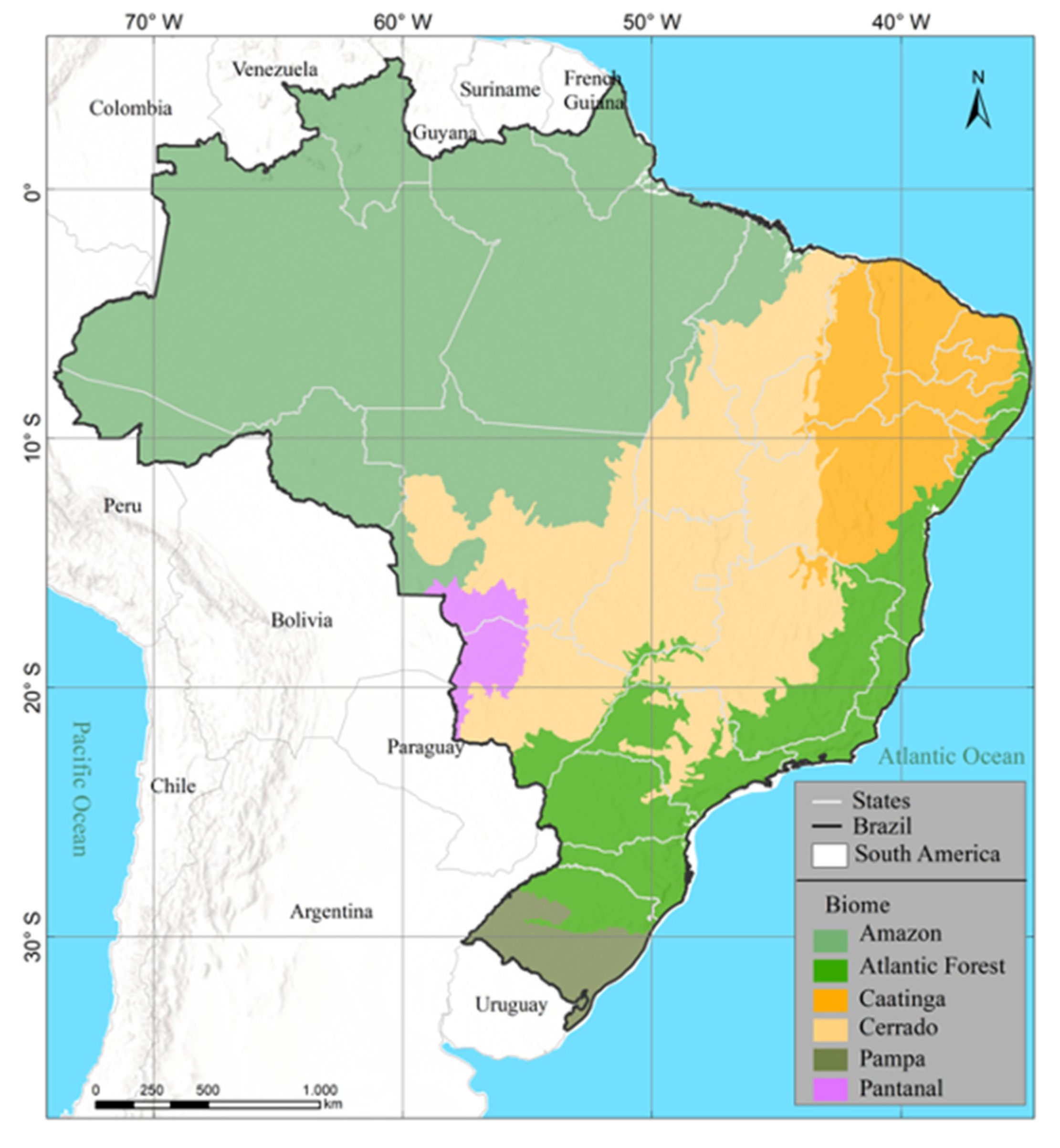
Brazil is one of the richest biodiversity countries in the world [7] with six unique biomes: Amazon, Atlantic Forest, Caatinga, Cerrado, Pampa and Pantanal. These biomes possess large carbon stocks in their forest [8] and soils [9], and additionally possess the largest global reserves of freshwater [10]. On the other hand, this country is one of the world’s producers of agricultural commodities and it has been a major contributor to LULC changes from greenhouse gas (GHG) emissions at the global scale [11,12].

Deforestation for pasture and agriculture expansion, infrastructure development, cities, and political and financial incentives to land occupation are the main drivers of LULC changes in the Brazilian biomes, affecting biodiversity, water resources, carbon emissions, regional and local climate [13]. Currently, the biomes undergoing more pressure on the original land cover are the largest ones, the Amazon (419 Mha, i.e., 49% of the country) and Cerrado (203 Mha, i.e., 23% of the country) [14,15]. However, the Atlantic Forest (111 Mha, i.e., 13% of the country) is the Brazilian biome that suffered the most extensive LULC change in the past, dating back to colonial history in the sixteenth century [16,17]. This biome is highly fragmented by roads and urban centers [18], and immersed in a large agriculture matrix, resulting in 11.7% of old secondary forest cover (i.e., >30 years) [19]. The semi-arid Caatinga biome (84 Mha, i.e., 10% of the country), located in the northeast region of Brazil, is considered the Brazilian biome that has been most altered by LULC change [20], being mainly covered nowadays by secondary growth forests [21,22]. Similarly to the previous ones, the Pantanal biome (15 Mha, i.e., 1.7% of the country) is likewise under high conversion pressure. Cattle ranching and sugarcane expansion are driving the suppression of its natural vegetation grassland and extensive wetlands [23,24]. Last, but not least, the Pampa biome (17 Mha, i.e., 2% of the country), is located in the southernmost region of the country, comprised mostly of natural grasslands with shrub trees and rocky outcrops [25]. Cattle ranching and agriculture have altered most of the natural grassland of this biome [26], and it has been considered a neglected biome due to inadequate protection and conservation policies [27,28,29].

Spatially explicit information on the historical trajectories of LULC in Brazil is key to inform the planning and the sustainable management of natural resources, policy formulation, among other societal applications. Nevertheless, as consequence of governmental policies and funding focused on the biomes that host most of the remaining Brazilian natural vegetation under threat, maps for measuring the historical extent and intensity of LULC change often exist for the Amazon and Cerrado biomes, and are scarce and/or lack adequate spatial and temporal resolution in the other biomes. Examples of mapping efforts include the Probio project from 2002 by the Brazilian Ministry of Environment, the National Inventory from 1994, 2002 and 2010 [30] and the Brazilian Institute of Geography and Statistics (IBGE) LULC maps from 2000, 2010, 2012, 2014, 2016 and 2018. These national mapping initiatives mostly used a combination of image pre-processing and enhancement, followed by labeling and digitizing classification based on visual interpretation, which is time consuming and prohibitively expensive for annual mapping and the reconstruction of long (i.e., >30 years) historical LULC information. Global LULC products varies from coarser to fine spatial resolution (i.e., 1 km to 30 m) satellite data and cover shorter time series intervals [31,32,33]. Additionally, global maps have none or little involvement of local experts in the production of LULC maps, requiring further assessment by experts at the national level [34].

The open access of Landsat archive [35,36,37], the new cloud computing Google Earth Engine (GEE) platform with machine learning algorithms [38,39], and a network named MapBiomas (https://mapbiomas.org/), including experts in remote sensing and computing, data science, and biomes, allowed us to reconstruct annual LULC classification at 30 m spatial resolution between 1985 and 2017. Our research network implemented image-processing algorithms in GEE to pre-process all Landsat images and normalize them to train a random forest classifier to map LULC classes of all biomes in Brazil. Massive cloud computing permitted the quick and automatic processing of a large set of images covering 33 year-long time series made of annual mosaics covering the entire extension of Brazil. The application of a cloud and cloud-shadow masks algorithms allowed to overcome Landsat scene cloudiness limitation for mapping LULC as previously reported elsewhere [40].

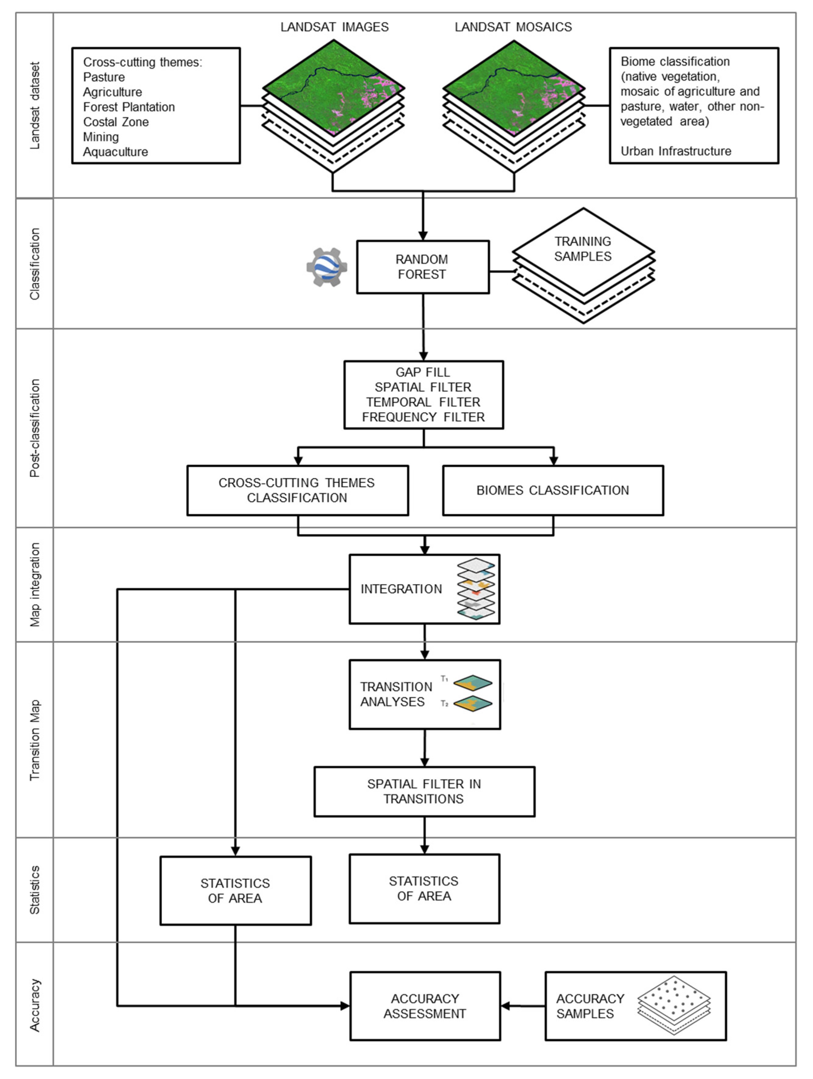
The objectives of this paper were threefold. First, we aimed at presenting how we reconstructed the annual time-series of LULC maps for all the Brazilian biomes between 1985 and 2017, by combining Landsat data, GEE, machine learning and a network of local experts, in a concept of progressively evolving LULC map collections. The second objective was to assess the extent, rates and main drivers of LULC change in the Brazilian biomes between 1985 and 2017 using the LULC time-series produced. The last objective was to present the MapBiomas image processing and classification protocol which maps the main land cover classes separately for each biome and common cross-cutting land use themes (i.e., pasture, agriculture, coastal zone, and urban infrastructure) followed by the integration of the LULC map products. We then demonstrated that the proposed protocol of MapBiomas is a step-wise learning process from local experts and feedback from users to improve the annual LULC maps. We also discuss the current applications of this free open access dataset to science, policy and monitoring LULC change in Brazil, as well as the remaining uncertainties and challenges of our LULC mapping approach.

2. Materials and Methods

2.1. Study Area and LULC Approach

Brazil is a megadiverse country, the largest in South America. Its vast territory occupies more than 851 Mha embracing six unique biodiversity-rich biomes named Amazon, Cerrado, Caatinga, Pampa, Pantanal and Atlantic Forest (Figure 1). These biomes have distinct characteristics in terms of vegetation structure and composition, soil physical and chemical characteristics, water availability, biodiversity with endemic ecosystems, climate conditions and land use activities. A long history of land use activities has transformed the original land cover characteristics of these biomes as summarized in

Table 1. Land cover and land use characteristics of the Brazilian biomes.

Biome	Area (Mha, %)	Land Cover	Predominant Land Use
Amazon	419 (49.29%)	Evergreen forest, with enclaves of savanna, natural grassland, and extensive wetlands and surface water, with almost 20% of the forested areas biome cleared.	Cattle ranching, agriculture, mining, logging and non-timber forestry production.
Atlantic Forest	111 (13.04%)	Isolated forest fragments covering 7–10% of the biome, mostly old secondary growth, surrounded by croplands, pasture, forest plantation, urban and infrastructure.	Agriculture, cattle ranching, urban, forest plantation, artificial water reservoir.
Caatinga	84 (9.92%)	Woody and deciduous forests, with at least 50% of the original converted.	Agriculture, cattle ranching, smallholder livestock production, non-timber forestry, and urbanization.
Cerrado	203 (23.92%)	Mosaic of savannas, grasslands and forests, 50% of the native vegetation cover has already been converted.	Agriculture, cattle ranching, artificial water reservoir and timber exploitation for coal production.
Pampa	17 (2.07%)	Natural grassland (Campos), with scattered shrub and trees, rock outcrop formations.	Agriculture, livestock production (in natural grasslands), forest plantation, and urbanization.
Pantanal	17 (1.76%)	Savanna, grassland and wetland.	Agriculture and cattle ranching.

.

We produced the annual historical maps of LULC between 1985 and 2017 separately for each biome and cross-cutting themes (i.e., pasture, agriculture, coastal zone, mining and urban infrastructure). Then, the maps of biomes and cross-cutting themes were integrated annually. The building blocks of the image-processing protocol to reconstruct annual LULC maps is presented in detail in the sub-sections (Figure 2), and the methodological details for each biome and themes can be found in the Supplementary Material (S1 and S2 Appendices). This is a key element of the MapBiomas LULC protocol which enables the mapping of complex and heterogeneous ecosystems.

2.2. Land Use and Land Cover (LULC) Classification

Defining a classification system remains a challenge for remote sensing and land ecosystem studies, especially for harmonizing different map products [42]. Land cover refers to the Earth’s surface characteristics, while land use is linked to human interactions with land surfaces [43]. The MapBiomas classification scheme is a hierarchical system with a combination of LULC classes compatible with the Food and Agriculture Organization (FAO) [44] and IBGE [45] classification systems (Table S2). At Level 1, there are six classes: forest (1), non-forest formation (2), farming (3), non-vegetated area (4), water (5) and not observed (6). The forest class includes old growth mature forest (i.e., >30 year-old), early stage (i.e., 5–15 year-old) and advanced secondary growth (i.e., 15–30 year old) forests, pristine forests that have not undergone anthropogenic conversion, savanna woodlands, mangroves and forest plantation. Farming constitutes a land use class for areas dedicated to growing crops and raising livestock. We also attempted to separate farming from non-forest natural formation and non-vegetated area at this first level, but made no attempt to separate natural forest cover from forest plantation, which is a land use activity (

Table 2. Land cover and land use classification system for MapBiomas in Brazil.

Level 1	Level 2	Level 3	Description
Forest	Natural Forest Formation	Forest Formation	Vegetation types with a predominance of tree species with high-density continuous canopy, areas that were disturbed by fires and/or logging, and forest resulting from natural regrowth.
		Savanna Formation	Vegetation types with a tree layer varying in density, distributed over a continuous shrub-herbaceous layer.
		Mangrove	Dense and evergreen forest formation often flooded by tide and associated with the mangrove coastal ecosystem.
	Forest Plantation		Planted tree species for commercial use.
Non-Forest Formation	Non-Forest Formation in Wetland		Floodplain with fluvial and lake influence, subject to periodic or permanent flooding, located along watercourses and in lowlands areas that accumulate water, with herbaceous shrub vegetation and/or arboreal and pioneer formations, and marshes (marine influence).
	Grassland Formation		Vegetation type with a predominance of herbaceous stratum, including patches with a well developed shrub-herbaceous stratum.
	Salt flat		“Apicuns” or salt flats are formations often without tree vegetation, associated to saline and a less flooded area in the mangrove, generally in the transition between this area and the continent.
	Other Non-Forest Formation		Natural grasslands, Savanna, Park Savanna, Steppe Savanna, Woody-Grassland Savanna, “Campinarana” in the Amazon biome.
Farming	Pasture		Pasture areas, natural or planted, related with farming activity. In particular, in the Pampa and Pantanal biomes, part of the area classified as Grassland Formation also includes pasture areas.
	Agriculture	Annual and Perennial Crop	Areas predominantly occupied by annual crops and in some regions (mainly in Northeast) with the presence of perennial crops.
		Semi-perennial Crop	Areas cultivated with the sugarcane plantation.
	Mosaic of Agriculture and Pasture		Farming areas where it was not possible to distinguish between pasture and agriculture.
Non-Vegetated Area	Beach and Dune		Sandy areas, with bright white colour, where there is no vegetation predominance of vegetation of any kind.
	Urban Infrastructure		Urban areas with a predominance of non-vegetated surfaces, including roads, highways and constructions.
	Rocky Outcrop		Naturally exposed rocks in the terrestrial surface without soil cover, often with partial presence of rock vegetation and high slope.
	Mining		Areas related to large mineral extraction, with clear soil exposure due to heavy machinery. Only areas belonging to National Department of Mineral Production’s (DNPM) chart (SIGMINE) were considered.
	Other Non-Vegetated Area		Non-vegetated surface areas (infrastructure, urban areas or mining) not mapped into their classes, and exposed soil areas (mainly sandy soil) not classified as grassland formation or pasture.
Water	River, Lake and Ocean		Rivers, lakes, dams, reservoir and other water bodies
	Aquaculture		Artificial lakes, where aquaculture and/or salt production activities predominate
Not Observed			Areas blocked by clouds or atmospheric noise, or with absence of ground observation masked out from analysis.

and Table S2).

Level 2 has 12 classes that also have a combination of LULC classes (Table 2). The Forest Level 1 class is broken down into two sub-classes: natural forest formation (1.1) and forest plantation (1.2). Then, non-forest natural formation is divided into wetland (2.1), grassland (2.2), salt flat (2.3) and other non-forest natural formation (2.4); farming into pasture (3.1), agriculture (3.2) and mosaic of agriculture and pasture (3.3); and the non-vegetated area into beach and dune (4.1), urban infrastructure (4.2), rocky outcrop (4.3), mining (4.4) and other non-vegetated area (4.5). The Water Level 1 class was not sub-classified into the Level 2. Only the Forest class goes down to Level 3. The natural forest formation was sub-classified into forest formation (1.1.1), savanna formation (1.1.2) and mangrove (1.1.3).

The MapBiomas LULC Classification System can be linked to other international and national classification systems [44,45]. A detailed description of the MapBiomas LULC Classification and the correspondence with other systems is available in the Table S2. The classification method for implementing the MapBiomas LULC Classification System is also hierarchical, combining the different methods that are described below. Because of that, we defined the prevalence rules to combine the classification results obtained with different methods in order to obtain the final LULC classes (Table 2).

2.3. Remote Sensing Dataset

The satellite imagery dataset used in the MapBiomas project was composed by the Thematic Mapper (TM), Enhanced Thematic Mapper Plus (ETM+) and the Operational Land Imager (OLI) Landsat sensors, on board Landsat 5, Landsat 7 and Landsat 8, respectively. MapBiomas used Collection 1 Tier 1 from [46] with the original digital numbers (DN) converted to top of the atmosphere (TOA) reflectance. The Landsat Tier 1 imagery data were already orthorectified based on ground control points and digital elevation model. The Landsat Collection 1 Tier 1 was orthorectified accounting for pixel co-registration and the correction of displacement errors with the pixel spatial resolution of 30 m, and is normalized to TOA reflectance, making it suitable for LULC change analysis [47]. The Landsat Collection used in this study was accessible and processed through Google Earth Engine [38].

2.3.1. Pre-Processing

The mapping unit adopted in the MapBiomas project was defined based on the subdivision of the International Chart of the World to the Millionth on the 1:250,000 scale. Each tile covers an area of 1°30′ of longitude by 1° of latitude, totaling 558 tiles covering all the Brazilian biomes (Figure S1). Mapping tiles intercepting more than one biome were processed separately, with a classification legend, input and parameterization, specifically set for each biome and subsequently merged to the tile area in the post-classification step (explained later on).

The first pre-processing step was to build cloud-free annual tile Landsat mosaics yearly. Cloud and cloud shadow masks were applied to all Landsat scenes. For that, we used the temporal dark outlier mask (TDOM) [48] algorithm and the band quality assessment (BQA) information available in the Landsat Collection. The cloud-masked Landsat scenes, which are image data for specific dates and geographical locations, were selected in Google Earth Engine from the available Landsat archive and combined to produce annual temporal mosaics targeting specific periods of the year for each biome and sub-regions. This procedure warranted that optimal spectral contrast and separability amongst the LULC classes were obtained across the biomes. The Landsat mosaics were generated with statistical reducers (i.e., mathematical functions in Earth Engine), including median, standard deviation, minimum and maximum, among others. We used both Landsat mosaics and Landsat cloud-free scenes in our LULC random forest classification approaches, as described below and in the Appendix S1. These Landsat datasets are the basis to build input features for the classifiers, as described in the next section.

2.3.2. Landsat Feature Space

The annual Landsat scenes produced in the pre-processing step were used to generate the feature space (i.e., variables) used as input for the random forest classifier. All cloud-free Landsat scenes acquired over the biomes in a given year were used to produce temporal annual mosaics with spectral bands and index, fractions and index from spectral mixture analysis (SMA), temporal index (based on median, min, amplitude and standard deviation reducers) and textural index. The images from the best period of each biome (Table S3) were used to produce median images. Each biome had the flexibility to define the optimal period of the year to build the annual mosaics, since the cloud condition and phenological behavior of the LULC varies across the biomes. Therefore, the annual image mosaics have a different reference period for each biome. We also tested the map accuracy with calibration training data to assess if the period selected for building the annual mosaics was optimum to increase the accuracy of LULC classes. Building the annual mosaics with a different time period in the year did not affect LULC annual change estimates because the reference period of each biome is the same over time, allowing to build a single annual product at that level (Table S3).

After building the annual mosaics, the next step was to build the feature space for the random forest classifier. For that, we used the compositional, spectral, temporal and textural information extracted from the image annual mosaics and from all cloud-free pixels within the year. Fractional information was obtained with spectral mixture analysis (SMA; Tables S4 and S5) which was also used to calculate additional SMA indices such as the normalized difference fraction index (NDFI) [49]. The NDVI values of all cloud-free pixels of all images in each year were divided into quartiles, and then the median values of the highest quartile were considered the wet season image and the lowest one the dry season image. Reducers of minimum, maximum, difference and standard deviation were used in cloud-free pixels of all images in each year to produce the temporal index. Finally, an entropy function was applied in a 5 × 5 window around each pixel to produce the texture index in the Green band. A total of 104 features were available for each biome to select the best features. The feature dataset used by each biome is presented in the Supplementary Material (Appendix S1 and Table S6).

The temporal mosaics procedure described above is not optimal to separate all LULC, especially agriculture and pasture and non-forest formations due to seasonal changes. To overcome this limitation, some classes were classified separately, as cross-cutting themes. These classes included: pasture, agriculture, forest plantation, urban infrastructure, and mining. Each cross-cutting theme (used a specific classification approach with all cloud-free Landsat scenes available yearly, or a temporal mosaic for specific intra-annual period, to highlight the seasonal change and better distinguish these LULC classes. Additionally, the feasibility to derive the 104 variables varied temporally and spatially due to data availability and cloud conditions. The areas affected by these factors, with less Landsat data, generally produced poorer classification results which were corrected using the temporal filtering approach. More information about the cross-cutting theme input images and their classification methods are provided in the Appendix S2.

2.3.3. Random Forest Classification

We used the random forest classifier available in Google Earth Engine for LULC classification [38]. The number of trees in the random forest classifier varied from 50 to 100 iterations (Appendix S1 Table B; Appendix S2). The number of features selected was the default value for this parameter (i.e., mtree which is given by the square root of the number of features as defined for each biome).

For training the random forest classifier, we applied two approaches. For the Amazon biome, we combined existing land cover maps to randomly select and automatically assign the land cover classes to the training samples. We extrapolated the land cover class assigned to the training sample for the years that did not have land cover maps from other sources. Image analysts inspected Landsat color composites of these years and reassigned the correct land cover to the training samples. For the other biomes, we built training samples for the random forest classifier using a previous MapBiomas Collection 2.3 as a reference to identify stable land cover classes; i.e., pixels with no change in land cover over the timespan of this map collection (2000–2016). The stable land cover classes are the ones that did not change the pixel LULC class between 2000 and 2016. This map with stable land cover classes was used to randomly select samples and assign the LULC class to training samples. For the years 1985–1999 and 2017, which completes the LULC Collection 3.1 of this study, we extrapolated the stable land cover classes, assessed possible land cover change, and kept the LULC class if no change was observed. The cross-cutting themes also used a combination of stable samples, reference maps and image interpretation to build their training samples. More details about the procedure to build training samples are presented in the Appendix S1 and Table S6.

2.3.4. Post-Classification Filters and Map Integration

The final classification result for each map tile consisted of three products: (a) classification (no post-processing), (b) classification after applying spatial and temporal filters and (c) post-filter, integrated classification resulting from combining with cross-cutting themes following empirically defined prevalence orders. The first post-classification action was the application of spatial and temporal filters to the maps generated in the LULC classification step. The application of these filters removed classification noise and disallowable LULC class transitions. The temporal filter was also used to fill the information gap due to the cloud. These post-classification procedures were implemented in the Google Earth Engine platform and are described in more detail below.

2.3.5. Spatial Filter

The spatial filter segmented and indexed the classes of each collection into contiguous regions [50], which were subsequently identified and reclassified based on the following criteria: areas less than or equal to half a hectare (i.e., approximately 5 pixels) were reclassified based on the majority of the neighboring classes. For instance, a patch belonging to a given class of up to 5 pixels was first identified along with its neighboring pixels; this patch was then reclassified as the predominant class value of the neighboring pixels. This process was applied to all segments of the LULC classes selected for filtering, which corresponds to the minimum mapping unit of MapBiomas Collection 3.1. Spatial filters applied in each biome and cross-cutting theme are described in the Appendices S1 and S2.

2.3.6. Temporal Filter

The temporal filter seeks to identify and correct the class transitions that are expected along a series of consecutive years (i.e., 3 to 5), as well as to fill in pixels with no data caused by cloud cover [50]. For example, a pixel classified as non-forest in a given year ti (where i = 2008, 2009, …, 2015), and forest in year ti1 and ti+1, was reclassified as forest for the year ti. Several transition rules were defined and applied to be used in the temporal filter for each biome to deal with specific phenological and land use transitions. Temporal filters applied to each biome and cross-cutting theme are presented in the Appendices S1 and S2.

2.3.7. Map Integration

The biome products of digital classification after temporal filter application, for each of the 33 years in the period 1985–2017, were then integrated with the cross-cutting themes, by applying a set of specific hierarchical prevalence rules (Table S6). The integration process was made on a per pixel basis. A spatial filter similar to the one described above was applied in the integrated maps to remove the isolated classes with less than half a hectare, as well as the noise resulting from any Landsat data misregistration.

2.3.8. LULC Transitions

Transition classes represent LULC change measured by the annual pixel-to-pixel class difference between 1985 and 2017. A similar spatial filter described in the Section 2.3.5 was applied in the transition maps to remove spurious isolated class transitions. The aim of the LULC transition filter is to eliminate single pixels or streams of pixels on the border of different classes derived from the created transition maps. The general rule applied in this filter was to remove from the transition classes’ single isolated pixels and streams of up to five pixels along the border of transition classes.

2.4. Accuracy Assessment and Area Estimation

Accuracy assessment analysis and area estimation were performed based on ~75,000 independent samples (named reference dataset) at the Landsat pixel level for each one of the years from 1985 to 2017 in all of Brazil (Appendix S3). These samples were generated by a stratified random sampling, which considered 127 regular strata (resulting from the spatial aggregation of neighbors tiles from International Charts of the World to the Millionth on the 1:250,000 scale), a confidence interval of 95%, and a maximum standard error of 5% to establish the sample size for each stratum, following the good practices proposed by [51,52]. In order to increase the number of samples in heterogeneous landscapes, we stratified the samples proportionally to six slope classes (see the Appendix S3 for details).

Each sample (i.e., Landsat pixel) was inspected by three independent interpreters, and in case of disagreement among interpreters, a senior interpreter assigns the final LULC class of the pixel. This evaluation was performed using the Temporal Visual Inspection web application (TVI—tvi.lapig.iesa.ufg.br), developed by the Laboratório de Processamento de Imagens e Geoprocessamento (Lapig).The TVI application allowed the evaluation of all LULC classes using at least two Landsat images per year, the Moderate Resolution Imaging Spectroradiometer (MODIS) vegetation index, precipitation time-series, and high-resolution imagery available in Google Earth. Accessing all these datasets for each sample through a graphical user interface of TVI with satellite image color composites to provide texture and contextual information, spectrum-temporal graphs to assess phenology of LULC class, and higher spatial resolution imagery, allowed the interpreters to evaluate and differentiate the LULC classes (Table 2). Additionally, all TVI interpreters were trained by experts from each of the Brazilian biomes, in order to establish the interpretation criteria for all the LULC classes mapped by MapBiomas.

Subsequently, we used a majority agreement rule, which considers the LULC class assigned by the majority of the interpreters as the final one to the reference sample. Finally, a classification error matrix was created and several metrics (i.e., global user and producer accuracies, quantity and allocation disagreement) were calculated for each year, class and biome, following a standard good practice protocol [51]. Then, we calculated the unbiased area estimation (using the sample weight obtained with our reference sample dataset), classification error matrix, and estimated user, producer’s and global accuracies, and quantity disagreement and allocation disagreement for each year, class and biome following a standard good practice protocol [51] (see Appendix S3 for details).

3. Results

3.1. LULC Map Accuracy

We generated 33 annual LULC maps for Brazil with Landsat data from 1985 to 2017 using Google Earth Engine at 30 m pixel resolution. First, we presented the temporal trends of the five main LULC classes including forest, non-forest formation, farming, non-vegetated area and water (

Table 3. Summary statistics for Class Level 1 for 1985 and 2017 and LULC area change between these years.

LULC Class (Level 1)	1985		2017		Area Change
	Area (Mha)	Area (%)	Area (Mha)	Area (%)	Mha	(%)
Forest	600.0	70.5	539.0	63.3	−61.0	−10
Non-Forest Formation	63.6	7.5	57.9	6.8	−5.7	−9
Farming	172.0	20.3	238.0	27.9	66.0	38
Non-Vegetated Areas	2.2	0.3	3.1	0.4	1.00	44
Water	12.5	1.5	13.5	1.6	1.00	8

, Figure 3). At Level 1, the LULC mapping product presented 89.13% of global accuracy with 9.21% of allocation disagreement and 1.66% of area disagreement (

Table 4. Overall average accuracy, standard error and disagreement by area and allocation at LULC classes in Levels 1 and 2 in each biome and Brazil between 1985 and 2017.

Level 1
Region	Overall Accuracy	Standard Error	Disagreement
			Area	Allocation
Brazil	89.13%	0.07%	1.66%	9.21%
Amazon	95.13%	0.09%	3.01%	1.86%
Atlantic Forest	87.30%	0.21%	1.47%	11.23%
Caatinga	80.03%	0.23%	1.13%	18.84%
Cerrado	81.40%	0.17%	4.71%	13.89%
Pantanal	73.17%	0.65%	15.68%	11.14%
Pampa	81.25%	0.54%	9.76%	9.00%
Level 2
Region	Overall Accuracy	Standard Error	Disagreement
			Area	Allocation
Brazil	87.91%	0.10%	4.42%	7.67%
Amazon	95.03%	0.09%	3.35%	1.62%
Atlantic Forest	83.25%	0.32%	5.52%	11.23%
Caatinga	78.18%	0.26%	7.29%	14.53%
Cerrado	79.88%	0.22%	6.38%	13.74%
Pantanal	66.09%	0.69%	15.73%	18.18%
Pampa	79.46%	0.59%	10.96%	9.58%

). The Amazon biome had 95.13% average global accuracy, which was the highest accuracy at class Level 1, followed by the Atlantic Forest biome with 87.3%. The Cerrado, Pampa and Caatinga had an average global accuracy ranging from 81.4% to 80.03%. The Pantanal biome had the lowest average global accuracy at class Level 1 (73.17%). For the class Level 2, the average global accuracy for Brazil had a marginal reduction (87.91%), with the Amazon biome showing almost the same value (95.03%) obtained at class Level 1. The Pantanal and the Atlantic Forest biomes showed the largest decrease in average global accuracy at class Level 2, of 7% and 4%, respectively. The Caatinga, Cerrado and Pampa had an average decrease of 1.7% (Table 4). The overall accuracy had a standard error < 1%, implying that it did not vary over the annual time series. The classification accuracy for each year between 1985 and 2017 is available in the Figure S2 and Dataset S2.

We summarized the user’s and producer’s accuracy estimates by averaging them over the 33 years timespan of this study for the entire country (

Table 5. User’s and producer’s accuracy average and standard error for LULC classes Levels 1 and 2 between 1985 and 2017.

Level 1
LULC Class	User’s		Producer’s
	Accuracy	Standard Error	Accuracy	Standard Error
Forest	92.41%	0.04%	94.72%	0.05%
Non-Forest Formation	61.76%	0.15%	59.19%	0.15%
Farming	87.73%	0.10%	83.55%	0.10%
Non-Vegetated Area	92.54%	0.49%	62.95%	0.31%
Water	88.95%	0.42%	85.40%	0.40%
Level 2
LULC Class	User’s		Producer’s
	Accuracy	Standard Error	Accuracy	Standard Error
Natural Forest Formation	92.08%	0.04%	94.77%	0.05%
Forest Plantation	92.90%	0.52%	52.98%	0.27%
Non-Forest Formation in Wetland	56.46%	0.57%	53.39%	0.54%
Grassland Formation	49.91%	0.14%	59.61%	0.17%
Other Non-Forest Formation	83.88%	0.42%	53.13%	0.25%
Pasture	90.63%	0.14%	75.92%	0.12%
Agriculture	81.28%	0.25%	83.25%	0.25%
Urban Infrastructure	92.54%	0.49%	62.95%	0.31%
River, Lake and Ocean	88.95%	0.42%	85.40%	0.40%

). These estimates allowed to break down the overall accuracy reported for the country level (Table 4) into class levels. For class level 1, the user’s accuracy ranged between 61.76% and 92.54%, for non-forest formation and non-vegetated, respectively. The lower user’s and producer’s accuracy of non-forest formation LULC classes, such as wetlands and grasslands at class Level 2, can be explained by the spectral confusion with other LULC classes such pasture, agriculture and water with Landsat data. Understanding the spectral confusion amongst the LULC classes is crucial for the proper user of the MapBiomas dataset. Because of that, all the classification error matrices are available in the Datasets S1 and S2 and we built an interactive visual tool to explore this information in the MapBiomas dashboard (https://mapbiomas.org/en/accuracy-analysis).

3.2. LULC Spatial and Temporal Trends in Brazil

In 1985, the forest class, which also includes forest plantation, secondary forest and old growth forest with or without signs of degradation by fire, forest fragmentation or selective logging, covered 70.5% of the Brazil’s territory, with 600 Mha. The total extent of the farming class reached 172 Mha in that year, with the second largest extent of land cover (20.3% of the territory). The minority land cover classes in terms of extent were non-forest formation (63.4 Mha, 7.48%), followed by surface water with 12.5 Mha (1.47%) and non-vegetated area (2.17 Mha, 0.25%) (Table 3).

We estimated the annual area change in the land cover classes at Level 1 and captured their temporal trends between 1985 and 2017 (Figure 3, Table 3). The forest class was the one with the greatest reduction in area, with a conversion of 61 Mha or 10% of forest loss between 1985 and 2017. Non-forest formation, comprised mostly of grasslands, also had almost 10% of its areas reduced in this period, losing 5.7 Mha. On the other hand, farming expanded by 38% with an absolute area of 66 Mha, but not all farming advanced through forested regions, as we will explain in more detail below. The other classes, water and non-vegetated area also expanded their area relative to 1985 by 8% (1 Mha) and 44% (0.96 Mha), respectively (Table 3). The fastest rate of annual land change happened between 1985 and 2005, for forest loss and farming and water expansion (Figure 3). The non-forest formation and non-vegetated areas showed faster annual changes after the year 2000.

At the country level, the water class showed the lowest annual average percent change (0.17% per year; s ± 7.12%) with a more pronounced trend towards reducing surface water between 2010 and 2017 in the Caatinga and Cerrado biomes (Figure 4B). The Caatinga biome showed the highest rate of surface water shrinkage in the 2010s, with an annual average rate of −5.1% per year, followed by the Cerrado biome which showed five years in this decade with surface water reduction. Disregarding the outlier in 2011 (8.89% increase relative to 2010), the Cerrado biome showed a decreasing change in surface water. In the Amazon biome, we also detected a slight signal of surface water reduction in the 2010s. The Atlantic Forest and Pampa biomes also showed a minor trend towards an increase in surface water and higher variation over the time-series period. However, surface water had the lowest extent in the Pampa biome between 1985 and 1995. The Pantanal biome presented the highest variation of surface water exhibiting a twenty-year harmonic cycle (1985–2005) (Figure 4; Table S7). Since 2005, surface water has been increasing in the Pantanal biome (5% average per year).

Non-vegetated area was the LULC class with the smallest extent, but showed a rapid increase in area from 1985 to 2017 with an average expansion rate of 1.72% per year (s ± 10.2%) in the whole country (Figure 4B). We expected this temporal change because urban and infrastructure development increased in Brazil in this period. We were not able to estimate the statistical factors to adjust the area estimate of this class for the Pantanal biome because of the lack of reference data. The Amazon biome had the lowest average annual change for this class in the entire period (0.4% per year). Moreover, the Cerrado biome had a 2% increase per year in surface area for non-vegetated areas, and the Caatinga and Pampa near 2.5%. The Atlantic Forest showed an overall annual increase in non-vegetated areas with an annual average rate of 1.3% per year. The overall rate for the Amazon biome was a 0.4% increase, with a higher variation of change along the time-series (Figure 4B; Table S7).

The farming class also expanded between 1985 and 2017 at rate of 1.7% per year (s ± 3.8%) (Figure 4). The highest annual average rate of farming expansion was detected in the Amazon biome (4.6% per year), followed by the Pantanal (3.5% per year). For the Cerrado, Pampa and Caatinga, the expansion of Farming was at a lower pace, with an annual rate of 0.9%, 0.8% and 0.6% percent increase per year, respectively (Figure 4B). However, we observed higher rates of farming expansion between 1985 and 2005 in the Amazon, Pantanal and Cerrado biomes, at 6.7%, 5.1% and 1.3% yearly expansion, respectively. After 2005, the annual expansion of Farming in these biomes fell to 1.2% in the Pantanal, 1% in the Amazon, and 0.4% in the Cerrado (Figure 4A, Table S7).

The non-forested formation class showed an annual change of −0.34% per year (s ± 2.8%) between 1985 and 2017. The Atlantic Forest and the Pampa biomes showed the highest rate of shrinking with −0.83% and −0.68% per year on average, respectively. The remaining biomes had a lower annual average reduction of non-forested areas ranging between −0.06% per year in the Amazon and −0.2% in the Cerrado (Figure 4B).

Finally, the forest class diminished by 0.34% (s ± 2.76) between 1985 and 2017 at the country level. The Pampa and the Atlantic Forest showed an increase in forest cover in this period with an average rate of 1% (s ± 4.27) and 0.05% (s ± 0.63) per year, respectively. The other biomes had their forest cover reduced. The fastest annual rate of forest decrease happened in the Cerrado biome (−0.6%, s ± 0.56), followed by the Pantanal (−0.33%, s ± 1.77), Caatinga (−0.3%, s ± 0.53), and Amazon (-0.31%, s ± 0.22). However, in absolute terms, the Amazon region has lost much more forest area than the other biomes in Brazil (Figure 4A,B).

3.3. The Main LULC Change in Brazil

The spatial distribution of these LULC classes in 1985 and 2017 are shown in Figure 5, which was used for quantifying the main LULC change in this period. Breaking down these LULC classes to the class Level 2 revealed more unique temporal trends of these classes by biome. In Figure 6, we have the area estimate for 10 of 16 LULC classes at Level 2 (Table 2) per biome. The wetland class was mapped only in the Pampa and Pantanal biomes and the other non-forest formation (ONFF) in the Amazon and Atlantic Forest (Figure 6), totaling 2.9 Mha and 15.6 Mha in 1985, respectively (

Table 6. Land use and land cover change in Brazil in 1985 and 2017.

LULC Class Level 2	1985 (Mha)				2017 (Mha)				Total Change	Total Percent Change
	Min	Area Adjusted	Max	% Area Mapped	Min	Area Adjusted	Max	% Area Mapped
Natural Forest	573.2	598.9	624.7	70.4%	507.6	533.0	558.4	62.6%	−65.9	−11.0%
Forest Plantation	−0.5	1.6	3.6	0.2%	2.5	5.9	9.3	0.7%	4.3	277.0%
Wetland	2.7	2.9	3.2	0.3%	1.5	2.2	3.0	0.3%	−0.7	−22.9%
Grassland	31.4	45.2	58.9	5.3%	28.6	40.7	52.9	4.8%	−4.4	−9.8%
Other Non-Forest Formation	8.3	15.6	22.8	1.8%	7.6	14.9	22.2	1.8%	−0.7	−4.3%
Agriculture	16.8	18.9	21.0	2.2%	49.0	51.5	54.0	6.1%	32.6	172.5%
Pasture	82.4	98.1	113.8	11.5%	109.1	143.5	177.9	16.9%	45.4	46.2%
Mosaic of Agriculture and Pasture	32.1	55.3	78.6	6.5%	30.3	42.7	55.1	5.0%	−12.7	−22.9%
River Lake and Ocean	11.2	12.5	13.8	1.5%	12.2	13.5	14.8	1.6%	1.0	7.8%
Urban Infrastructure	1.0	2.2	3.4	0.3%	2.0	3.1	4.3	0.4%	1.0	44.6%

). These classes combined covered 2.1% of Brazil in 1985 and 2017, and both lost 0.7 Mha in this period (Table 6). The majority of wetland mapped lays in the Pantanal biome, and the other non-forest formation was almost evenly split in the Amazon and the Atlantic Forest.

In our classification scheme, the Forest Level 1 class is split into natural forest formation (NFF) and forest plantation at the classification Level 2. The NFF is sub-classified into forest and savanna formations (Table 2). The NFF class covered 69% (598.9 Mha) of the Brazilian territory in 1985. Between 1985 and 2017, 11% of the country’s the NFF were converted into other land cover types, resulting in a forest loss of 65.9 Mha. Despite the relative 277% growth of forest plantation in this period, we estimated only 6 Mha was in plantations in 2017 (Table 6). It was not possible to estimate the area of forest plantation over the entire timespan of this study (i.e., 33 years) because of the limited reference samples for applying the area adjustment protocol over many years, in the Amazon, Cerrado and Pampa biome. Therefore, the area of this LULC class remains highly uncertain.

The grassland class was mapped in all biomes except in the Amazon (Figure 6). The total area estimated of grassland in 1985 reached 45.2 Mha (5.3% of the Brazilian territory). We detected a loss of 4.4 Mha of this class between 1985 and 2017 (9.8% loss). The annual mapping uncertainty over the time-series was high in Cerrado, and much higher in the Pampa and Pantanal biomes, and no area estimate was obtained for the Amazon biome grasslands (Figure 6, Table 6).

The area of agriculture increased in all biomes, except in the Pantanal, where it was not possible to characterize its temporal trend because we were not able to estimate the annual area for the entire time-series (Figure 6). The total area of agriculture increased from 18.9 Mha to 51.5 Mha between 1985 and 2017, representing a 172.5% expansion of 32.6 Mha (Table 6). Most of this expansion happened in the Atlantic Forest, Cerrado and Pampa biomes, with the highest area uncertainty in the later one (Figure 6).

The pasture class showed different annual trends in the biomes with periods of continuing expansion (Amazon and Pantanal), stabilization after 1995 (Caatinga, Cerrado), and shrinking (Atlantic Forest). This class was not mapped in the Pampa biome because natural grasslands area is used for raising animals in this biome. Overall, the pasture area increased by 45.4 Mha in Brazil from 1985 to 2017 (Table 6, Figure 6). In four biomes (Atlantic Forest, Caatinga, Cerrado, and Pampa), 143.5 Mha were mapped as either pasture or agriculture, which were assigned in the mosaicking class (Table 6, Figure 6). This mosaic class was reduced from 55.3 Mha in 1985 to 42.7 Mha in 2017 (i.e., a loss of −22.9%). This result may indicate that it has become more feasible to reliably distinguish pasture from agriculture in more recent years, reducing the mapping uncertainty between them.

River, lakes and ocean (RLO), as well as urban infrastructure LULC classes had an increase in area between 1985 and 2017 of 1.0 Mha each (Table 6). The temporal variation is better depicted for the river, lakes and ocean in the Figure 4B and the results for each biome were presented in the previous section. The remaining LULC classes that were not discussed here are rare classes (i.e., have a small proportion of area and reference data, such as mangrove, salt flat, beach and dune, rocky outcrop). Considering this, we were not able to provide a reliable estimate of their area with Landsat imagery.

3.4. LULC Biome Transitions

We estimated that 63.5% of the Brazilian territory did not undergo change in its original land cover class from 1985 to 2017, totaling 540.7 Mha (

Table 7. Estimate of the area (Mha) of persistent land cover and land use classes in Brazil between 1985 and 2017.

Classes	Amazon	Atlantic Forest	Caatinga	Cerrado	Pampa	Pantanal	Brazil
Natural Forest Formation	323.4	20.7	31.6	67.0	0.7	4.3	447.7
Non-Forest Formation	6.2	1.0	1.4	13.9	2.3	1.6	26.5
Forest Plantation	-	0.2	-	0.2	-	-	0.4
Pasture	4.2	15.0	4.8	14.4	-	0.2	38.6
Mosaic of Agriculture and Pasture	0.1	2.6	0.5	0.3	-	-	3.5
Agriculture	-	5.8	0.5	3.2	1.0	-	10.5
Non-Vegetated Area	0.1	1.0	0.1	0.5	0.1	-	1.9
Water	7.6	1.3	0.3	0.7	1.6	0.2	11.6

, Figure 7A). These persistent LULC classes do not imply that there were no land cover degradation processes during the 33-year period of this study or no land cover regeneration. Changes in their structure and/or composition, usually associated with wood, non-timber product forest harvesting, and fires may have happened, but no effort to detect degradation processes has yet been applied at the country level. The majority of the areas with persistent LULC classes occurred in the Amazon biome, encompassing 40% (341.6 Mha) of the total area in Brazil that did not show land cover change in the timeframe of this study. Our analysis showed that 323.4 Mha in the Amazon biome, or 94.6% of the total LULC that did not change, was represented by natural forest formation (Table 7). The Cerrado biome had the second largest area with no LULC change (110.2 Mha; 11.8% of the entire country), of which 67 Mha were natural forest formation. In the Atlantic Forest, the persistent land cover made up of 47.6 Mha (9.1% of the country), with nearly 50% associated with agriculture and pasture. The Caatinga biome had 39.2 Mha of LULC classes mapped in 1985 continuing in the same classes in 2017, with 80% (i.e., 31.6 Mha) related to natural forest formation. The Pampa and Pantanal biomes showed 0.7% for the total area relative to Brazil with no change in LULC classes (Table 7, Figure 7A).

The remaining 36.5% (310.8 Mha) of the country area showed changes in LULC classes from 1985 to 2017. We defined five types of changes amongst the LULC mapped in this study: vegetation loss, vegetation gain, water–land transitions, shifting land use and vegetation dynamics (

Table 8. Estimate of the area (Mha) of land cover and land use changes in Brazil between 1985 and 2017.

Classes	Amazon	Atlantic Forest	Caatinga	Cerrado	Pampa	Pantanal	Brazil
Vegetation loss	42.8	9.4	11.0	34.6	3.0	1.6	102.4
Vegetation gain	21.5	12.2	17.1	25.8	5.6	3.9	86.1
Water-land transitions	5.0	0.8	0.8	1.1	0.3	0.7	8.7
Shifting land-use	6.5	40.2	13.5	35.5	2.3	0.3	98.3
Vegetation dynamics	4.1	0.5	1.9	5.7	0.8	2.3	15.3

, Figure 7B).

The vegetation loss totaled 102.4 Mha, representing 33% of the total area that underwent LULC change between 1985 and 2017 (i.e., 310.8 Mha; Table 8). We discovered that most vegetation loss, which includes forest and non-forest formations, occurred in the Amazon (41.8%) and Cerrado (33.8%) biomes. To a lesser extent, in this category we had the following biomes: Caatinga (10.7%), Atlantic Forest (9.2%), Pampa (2.9%) and Pantanal (1.6%) (Table 8, Figure 7).

Shifting land-use was responsible for 31.6% of the total LULC change between 1985 and 2017 (Table 8), encompassing an area of 98.3 Mha. The Atlantic Forest and the Cerrado biomes contributed 40.9% and 36.1% to this change, respectively. The Caatinga (13.7%) and Amazon (6.6%) biomes contributed less to the shift amongst land use classes. In most cases, these changes were associated with farming, with agriculture replacing pasture. Finally, a shift in land use was much less pronounced in the Pampa (2.3%) and Pantanal (0.3%).

Vegetation gain reached an area of 86.1 Mha, or 10.1% of the Brazilian territory from 1985 to 2017. The Cerrado biome contributed to 30% (25.8 Mha) of the total area undergoing vegetation gain, followed by the Amazon biome with 25% (21.5 Mha) (Table 8) and the Caatinga biome with 19.9% (17.1 Mha). The Atlantic Forest gained 12.2 Mha (or 12.2% of the total vegetation gain) of area undergoing this process, with the great majority related to the newly forested region, mostly along riparian zones. We also detected 5.6 Mha and 3.9 Mha of vegetation gain in the Pampa and Pantanal biomes, respectively. A total of 15.3 Mha of the LULC changes in Brazil over the 33 years mapped in this study were associated with natural vegetation dynamics (1.8% of the country size), and 8.7 Mha (1%) with water to land transitions (Table 8, Figure 7B).

Since we did not generate reference data to assess the accuracy of the LULC transitions presented above, all the area estimates were based on pixel counting. Therefore, these results must be considered as a first attempt to characterize and measure LULC change in long time series in Brazil. We have not attempted to evaluate intermediary LULC change, which is the subject of another ongoing study.

4. Discussion

This is the first time that LULC change has been quantified in all Brazilian biomes with this degree of spatial detail (i.e., at 30 m pixel size) using +30-year time-series Landsat data. Until now, this LULC change information in Brazil was either restricted in space and time, covering a few biomes and short periods of time (e.g., [53,54,55]), or long time-series, but focusing on deforestation in the portion of one of the biomes [56]. Coarser spatial resolution remote sensing images have also been used to map LULC using Google Earth Engine covering all biomes in a single year [57], and global LULC products [31] are available with limited inputs from local experts. We did not attempt to investigate the level of spatial and temporal agreement between the MapBiomas LULC maps with the existing regional and global ones. This task is an ongoing effort of our research group, which requires the harmonization of LULC classification schemes, and spatial and temporal coherence amongst the LULC maps for undertaking the agreement analysis [58]. A recent study conducted by another research group compared their LULC maps, produced with PROBA-V imagery at 100 m pixel size, with our MapBiomas LULC map for 2015, resulting in a 69% agreement among the most representative LULC classes (i.e., forestland, shrubland, grassland, pastureland, cropland, water body used in the PROBA-V study) [57]. However, this study did not investigate which of these LULC products had the highest accuracy.

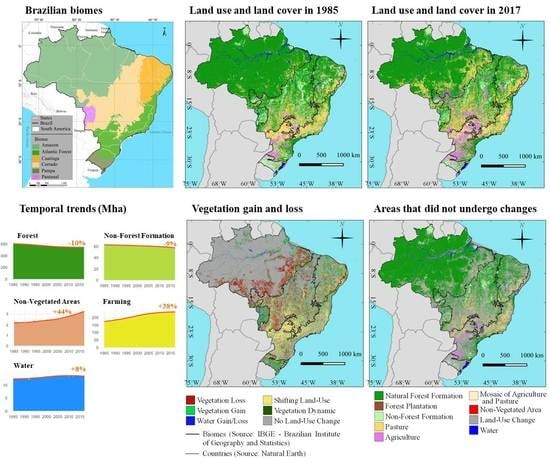
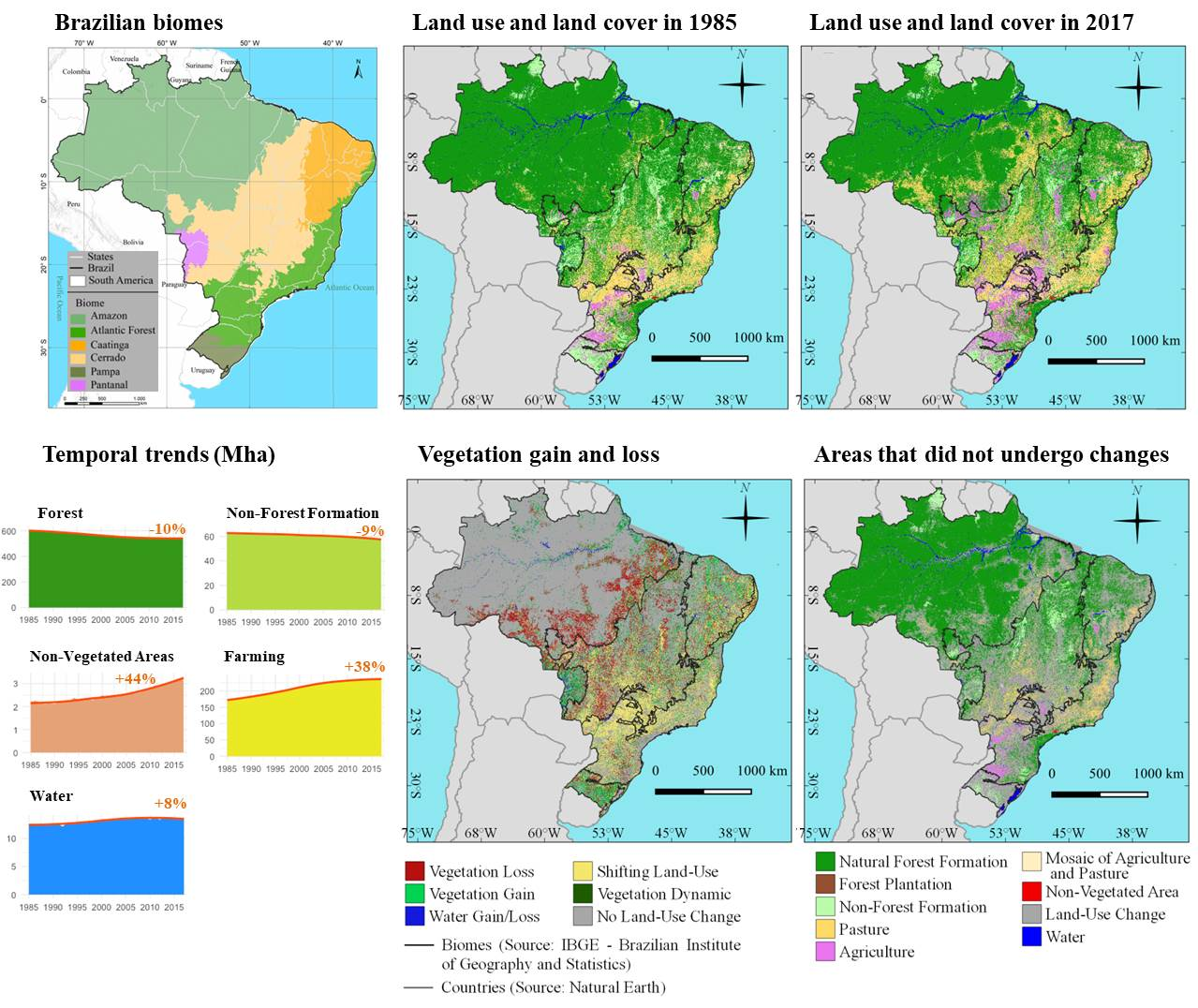
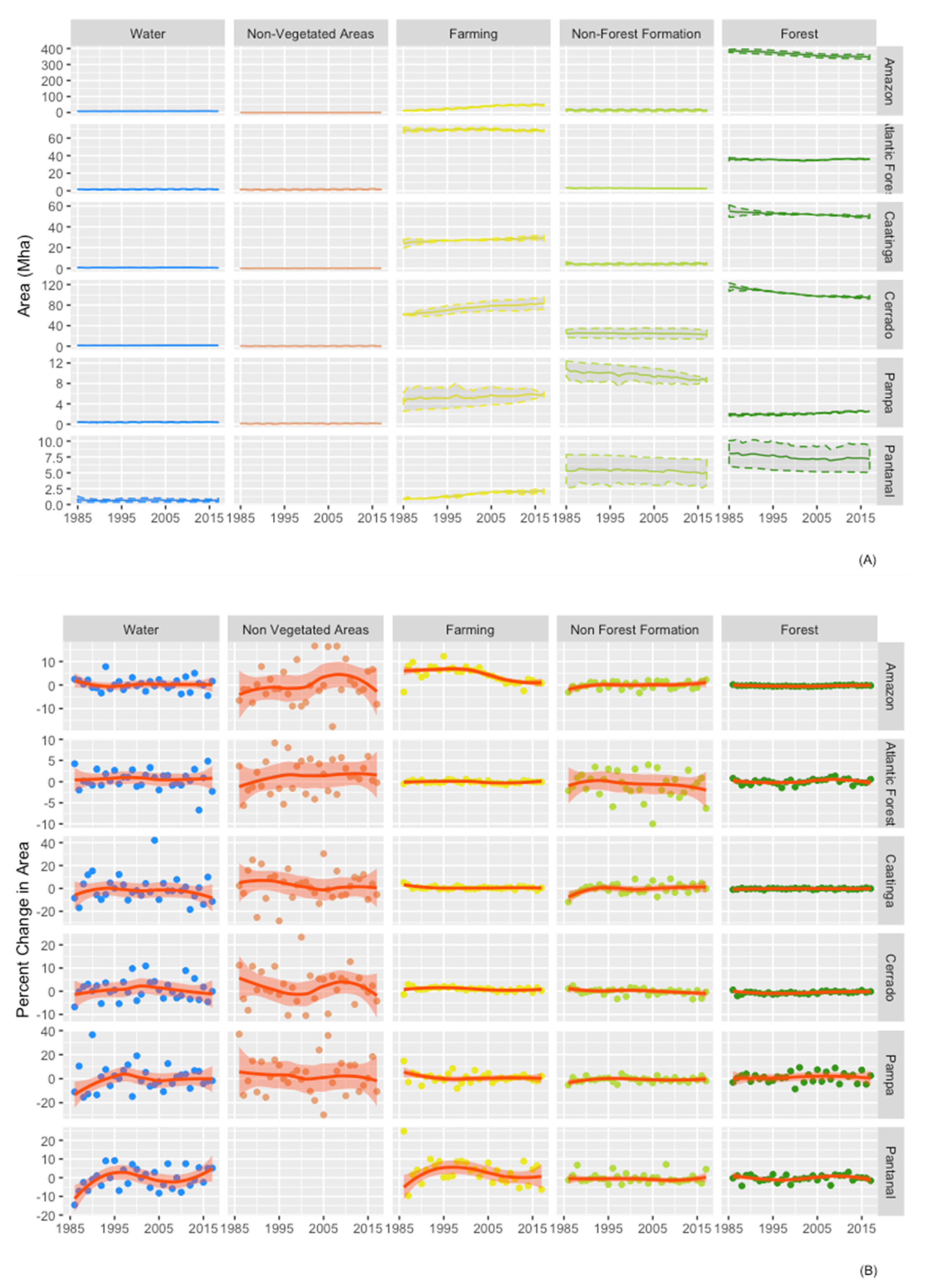
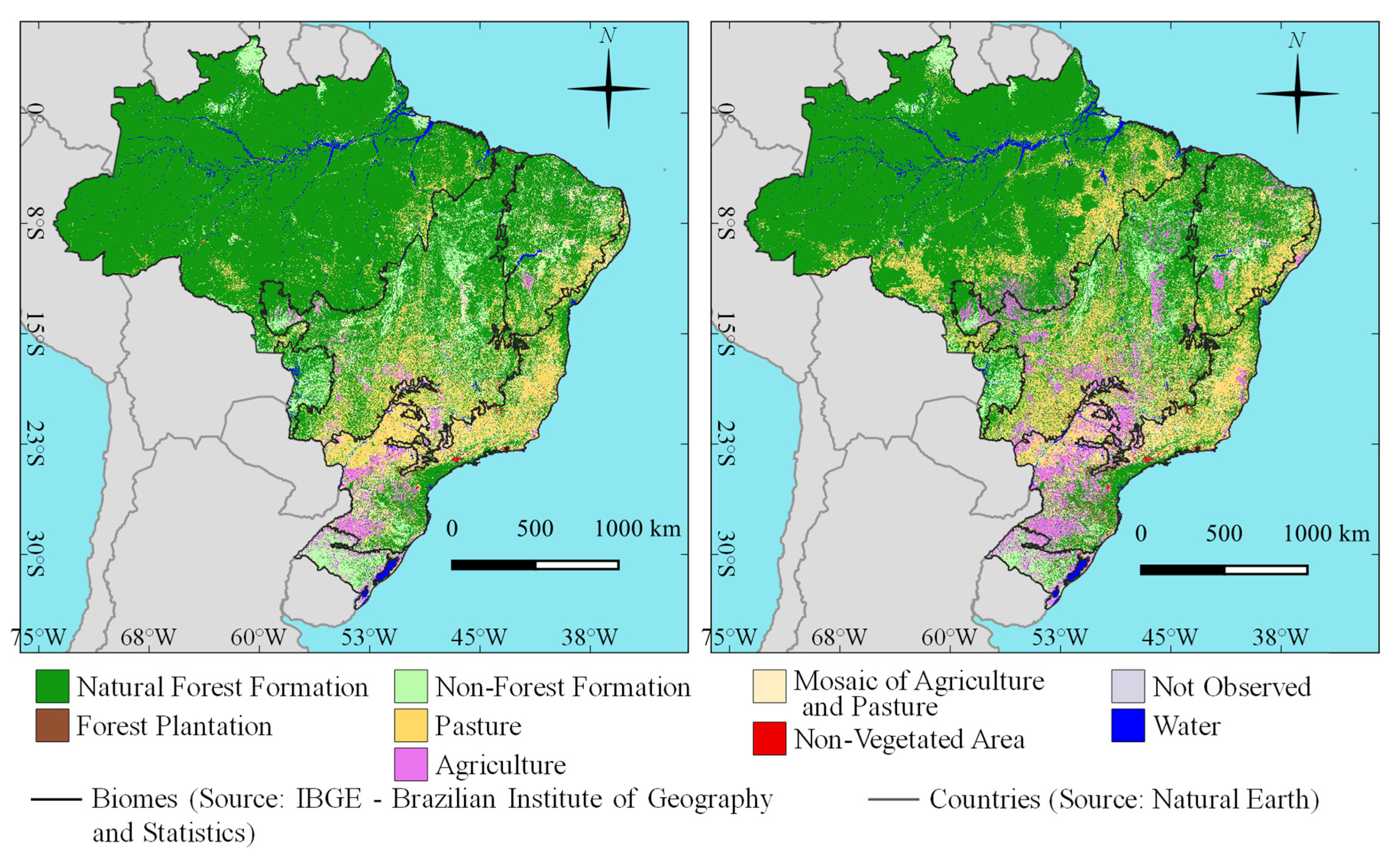
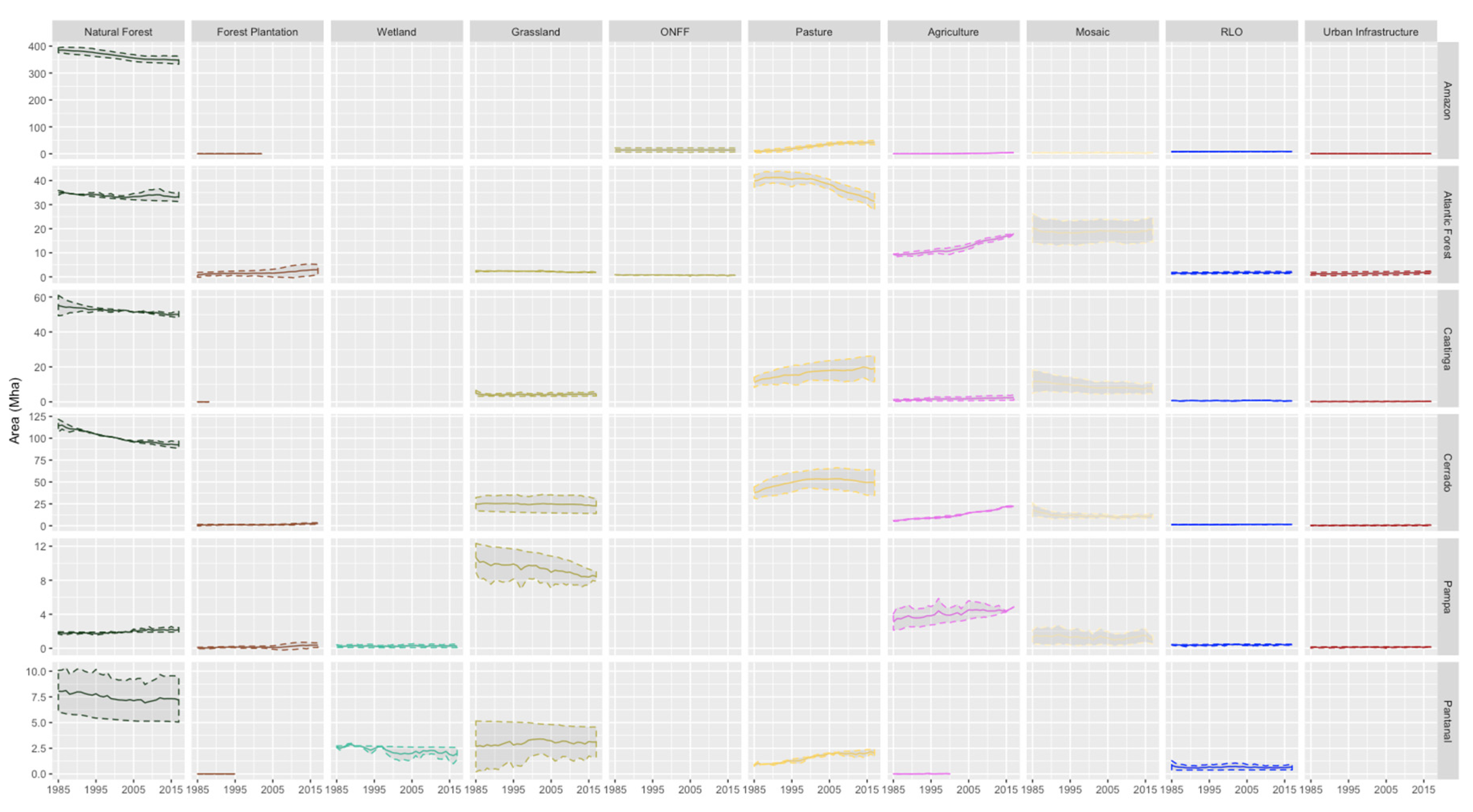
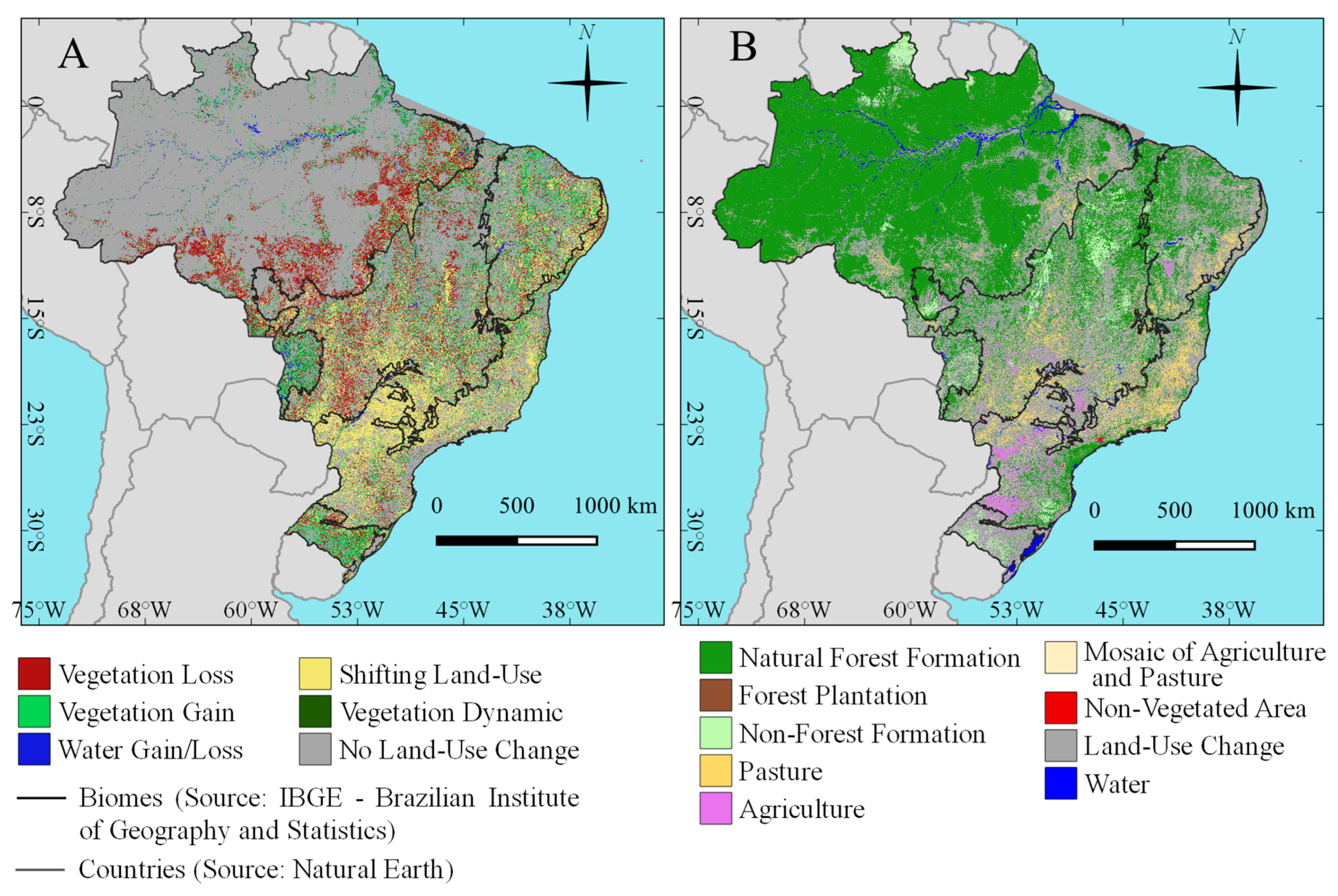
The LULC annual dataset presented in this study allowed numerous applications, such as the estimation of vegetation gain and loss, and the understanding of land cover drivers. Between 1985 and 2017, 38% of the Brazilian territory was modified by cattle ranching and agriculture activities, as well as infrastructure development, changing native forest and non-forest formations, indistinctly in all six biomes. Pasture expanded by 46% in the country, mainly in the Amazon and Pantanal biomes, while agriculture increased by 172%, mostly in the Atlantic Forest replacing old pastures and in the Cerrado biomes converting savanna and grasslands formations. Our LULC dataset revealed that 86 Mha of the converted native vegetation is undergoing some level of regrowth. The MapBiomas time-series also generated that, in the Amazon biome, secondary vegetation increased 12 Mha in 2017 [59], exceeding 45.5% to the area of primary deforestation mapped by the Brazilian monitoring system (PRODES) [60]. Thus, our LULC annual dataset goes beyond the existing LULC studies and monitoring systems and helps to fill the information and knowledge gaps in monitoring LULC dynamics in the country in the past three decades.

We built the LULC maps of this study iterating over map collections, such as that applied to MODIS global land cover products [33]. In the MapBiomas Collection 3.1, we had substantial improvement in the random forest classifier and built a robust reference dataset for accuracy assessment. The first Collection 1.0 was mainly developed to allow our research team, engineers and data scientist to port our existing classification algorithm and optimize Google Earth Engine LULC mapping in a short time-series (i.e., between 2000 and 2016). In the Collection 2 (which evolved until Collection 2.3), we were able to move from empirical decision trees based on hierarchical rules defined by analysts to a random forest machine learning algorithm. Empirical decision rules have an advantage of better understanding the variables and rules to map LULC classes, working well with a set of small classes [61]. However, as we increased the levels and numbers of LULC classes, empirical rules became complex, making human decision for partitioning the data into hierarchical binary classes unfeasible. To overcome this task, we adopted random forest in Collection 2.3 which evolved with unbiased training and accuracy assessment into Collection 3.1, using existing LULC maps from different sources to randomly select the training samples. Besides the iterative mapping collections, we implemented a flexible LULC mapping protocol which allows each biome to define the feature space and samples for training the random forest classifier (Appendix S1), as long as the biome maps can follow the map integration protocol to guarantee the spatial and temporal coherence along their transitional ecotone zones.

Yet, besides the gain in information brought by MapBiomas LULC Collection 3.1, there are still challenges and limitations to be overcome. First, overall accuracy was lower than 80% in highly seasonal and heterogeneous biomes (e.g., Cerrado, Caatinga, Pantanal and Pampa). The Amazon biome, with most of the land cover comprised by forest, had the highest overall mapping accuracy of 95%. However, less predominant LULC classes had lower accuracy in all biomes. For example, the spatial variability of native vegetation types and spectral similarity among LULC classes, such as grassland and pasture, are challenging to separate [62], even using hyperspectral images [63]. Second, the reference dataset used to assess the mapping accuracy was built based on the visual interpretation of Landsat color composites, and ancillary spectra-temporal time-series and higher resolution imagery data (when available). We were not able to estimate the classification uncertainty of our reference dataset, which is a task in course. Third, we still need to advance in the analysis of LULC transitions and estimate its uncertainties. In this study, we limited the LULC change analysis to a +30-year period for the LULC classes that had lower classification errors (Table 6, Table 7 and Table 8). Further investigation is necessary to understand the impact of LUCC classification error to estimate yearly change. Our research group is also exploring methods to understand the frequency of a pixel change to its LULC class and the number of times it happens [53,64]. Fourth, we recognize that the MapBiomas LULC mapping approach is complex because it involves different data inputs and algorithm parametrization for each biome, and some classes are mapped separately as a cross-cutting theme requiring post-classification integration from multiple classification results. As a single random forest classification failed to include all LULC (Table 2), it is likely that we will continue to use cross-cutting themes and post-classification integration of several maps and class prevalence rules to compose the final LULC. Rare classes in our classification schemes (e.g., beach and dunes, aquaculture, mining, salt flat, rocky outcrops) were penalized by the random forest classifier and tended to be under mapped, as pointed out in global mapping studies [33]. These rare LULC classes were impacted in our accuracy assessment analysis as well, showing high classification errors. As an alternative to overcome this issue, we balanced the training classes in our random forest algorithm by using published and accessible reference LULC maps for the Amazon biome, and by adding manually sampled areas that were under mapped in the other five biomes. However, the impact of rare classes persisted, leading us to analyze in this study the LULC dynamics of only the eight most predominant classes (Table 6). Finally, we will also attempt to separate agriculture from pasture in the mosaic class and improve the spatial and temporal consistency in some periods of time series in future MapBiomas Collections.

Several studies have already been published by the MapBiomas network to better understand the spatial-temporal LULC dynamics in Brazilian biomes focusing on specific LULC classes. For example, surface water dynamics in the Amazon region [65], Cerrado native vegetation change [62], mangrove [66] and pastureland dynamics and characterization over the whole country [67]. New research methods to explore and analyze LULC trajectories were applied to the Caatinga biome with the MapBiomas LULC time-series [68]. The Greenhouse Gas Emission and Removal Estimating System—SEEG [69] uses the LULC annual data to estimate the GHG emissions and removals for the land use sector in Brazil, which represents 44% of GHG emissions in 2018 (SEEG 7 available at https://seeg.eco.br/). Indeed, reducing the LULC uncertainty of the SEEG GHG estimates was the main reason for our research group to launch the MapBiomas Project.

All products, methods and tools of the MapBiomas Project are open access, transparent and publicly available in the internet (https://mapbiomas.org/) for non-commercial use. With open access data, it was possible to perfect the LULC maps with end-user feedback, which reached one hundred thousand users in 2019. Additionally, more than one hundred peer-reviewed research articles were published between 2017 and 2019 using the LULC maps of this project. Since the first MapBiomas Collection, the applications of this dataset keep growing in science including, for example, the assessment of conservation and biodiversity policies [70,71,72,73], climate change impact [74,75], and the mapping of human disease risks, including hantavirus [76], yellow fever [77], and Leishmania [78]. Therefore, these LULC maps presented in this study are already contributing to better inform the scientific community, policy makers and civil society organizations. In this study, we present an in-depth methodology and the processes used to build the MapBiomas collections, and a rigorous assessment of the map accuracy, which is required to support the existing and emerging scientific and societal applications of our LULC map collections. In addition, we are also advancing in the understanding of historical LULC dynamics in the Brazilian biomes and of the main drivers of change.

5. Conclusions

We reconstructed LULC time-series information over three decades in Brazil, based on Google Earth Engine cloud-computing, freely available Landsat data and a collaborative network of experts willing to share knowledge. Our LULC mapping protocol required breaking up the image classification per biome and cross-cutting themes, followed by the post-classification map integration rules. This process was required to account for the unique conditions of the biomes, including the phenological changes of LULC classes, the availability of Landsat data due to cloud conditions, and the history and intensity of land use. The accuracy assessment was used to define the optimum period of each biome using calibration data training embedded in the random forest classifier. Classifying separately cross-cutting classes (e.g., pasture, agriculture and urban infrastructure) was necessary to reduce spectral confusion in the random forest. The key element of our LULC approach is the post-classification integration protocol, which requires spatial coherence of the integrated maps along the biome boundaries. Finally, we decided to put the LULC maps openly available prior to the scientific publications, with a detailed description of the methodology. This allowed several scientific publications using our LULC dataset in Brazil and abroad, and getting feedback from the data users to improve our maps. Policy-makers are also using the LULC dataset to make, plan and assess public policies in the country. The MapBiomas collaborative initiative is also expanding to generate new LULC products in other countries, such as in the Pan-Amazonian countries (https://amazonia.mapbiomas.org/), Chaco region (https://chaco.mapbiomas.org/) and most recently in Indonesia. Based on MapBiomas experience in Brazil, involving local institutions and experts, and international partners, our LULC mapping protocol will likely expand to other countries contributing to support science and societal applications and better policy decisions.

References

1. DeFries, R.S.; Foley, J.A.; Asner, G.P. Land-use choices: Balancing human needs and ecosystem function. Front. Ecol. Environ. 2004, 2, 249–257. [Google Scholar] [CrossRef]
2. Lautenbach, S.; Kugel, C.; Lausch, A.; Seppelt, R. Analysis of historic changes in regional ecosystem service provisioning using land use data. Ecol. Indic. 2011, 11, 676–687. [Google Scholar] [CrossRef]
3. Walther, G.R. Community and ecosystem responses to recent climate change. Philos. Trans. R. Soc. Lond. B Biol. Sci. 2010, 365, 2019–2024. [Google Scholar] [CrossRef] [PubMed]
4. Ellis, E.C.; Goldewijk, K.K.; Siebert, S.; Lightman, D.; Ramankutty, N. Anthropogenic transformation of the biomes, 1700 to 2000. Glob. Ecol. Biogeogr. 2010, 19, 589–606. [Google Scholar] [CrossRef]
5. Verburg, P.H.; Crossman, N.; Ellis, E.C.; Heinimann, A.; Hostert, P.; Mertz, O.; Nagendra, H.; Sikor, T.; Erb, K.H.; Golubiewski, N.; et al. Land system science and sustainable development of the earth system: A global land project perspective. Anthropocene 2015, 12, 29–41. [Google Scholar] [CrossRef] [Green Version]
6. Butchart, S.H.M.; Walpole, M.; Collen, B.; Van Strien, A.; Scharlemann, J.P.W.; Almond, R.E.A.; Baillie, J.E.M.; Bomhard, B.; Brown, C.; Bruno, J.; et al. Global biodiversity: Indicators of recent declines. Science 2010, 328, 1164–1168. [Google Scholar] [CrossRef]
7. Myers, N.; Mittermeier, R.A.; Fonseca, G.A.B.; Kent, J. Biodiversity hotspots for conservation priorities. Nature 2000, 403, 853–858. [Google Scholar] [CrossRef]
8. Berenguer, E.; Ferreira, J.; Gardner, T.A.; Aragão, L.E.O.C.; De Camargo, P.B.; Cerri, C.E.; Durigan, M.; De Oliveira, R.C.; Vieira, I.C.G.; Barlow, J. A large-scale field assessment of carbon stocks in human-modified tropical forests. Glob. Chang. Biol. 2014, 20, 3713–3726. [Google Scholar] [CrossRef] [Green Version]
9. Bernoux, M.; Carvalho, M.D.S.; Volkoff, B.; Cerri, C.C. Brazil’s soil carbon stocks. Soil Sci. Soc. Am. J. 2002, 66, 888–896. [Google Scholar] [CrossRef]
10. Walter, E.H.M.; Kuaye, A.Y. Global Safety of Fresh Produce. In Global Safety of Fresh Produce; Woodhead Publishing: Sawston, UK, 2014; pp. 367–382. ISBN 9781782420187. [Google Scholar]
11. CAIT. CAIT Historical—Explore Historic Greenhouse Gas Emissions. Available online: http://cait.wri.org/ (accessed on 19 August 2020).
12. De Sousa-Neto, E.R.; Gomes, L.; Nascimento, N.; Pacheco, F.; Ometto, J.P. Land Use and Land Cover Transition in Brazil and Their Effects on Greenhouse Gas Emissions. In Soil Management and Climate Change: Effects on Organic Carbon, Nitrogen Dynamics, and Greenhouse Gas Emissions; Academic Press: Cambridge, MA, USA, 2017; pp. 309–321. ISBN 9780128121290. [Google Scholar]
13. Davidson, E.A.; De Araüjo, A.C.; Artaxo, P.; Balch, J.K.; Brown, I.F.; Mercedes, M.M.; Coe, M.T.; Defries, R.S.; Keller, M.; Longo, M.; et al. The Amazon basin in transition. Nature 2012, 481, 321–328. [Google Scholar] [CrossRef]
14. De Area Leão Pereira, E.J.; Silveira Ferreira, P.J.; de Santana Ribeiro, L.C.; Sabadini Carvalho, T.; de Barros Pereira, H.B. Policy in Brazil (2016–2019) threaten conservation of the Amazon rainforest. Environ. Sci. Policy 2019, 100, 8–12. [Google Scholar] [CrossRef]
15. Rausch, L.L.; Gibbs, H.K.; Schelly, I.; Brandão, A.; Morton, D.C.; Filho, A.C.; Strassburg, B.; Walker, N.; Noojipady, P.; Barreto, P.; et al. Soy expansion in Brazil’s Cerrado. Conserv. Lett. 2019, 12, e12671. [Google Scholar] [CrossRef]
16. Tabarelli, M. Effects of habitat fragmentation on plant guild structure in the montane Atlantic forest of southeastern Brazil. Biol. Conserv. 1999, 91, 119–127. [Google Scholar] [CrossRef]
17. Morellato, L.P.C.; Haddad, C.F.B. Introduction: The Brazilian Atlantic Forest. Biotropica 2000, 32, 786–792. [Google Scholar] [CrossRef]
18. Freitas, S.R.; Hawbaker, T.J.; Metzger, J.P. Effects of roads, topography, and land use on forest cover dynamics in the Brazilian Atlantic Forest. For. Ecol. Manag. 2010, 259, 410–417. [Google Scholar] [CrossRef]
19. De Rezende, C.L.; Uezu, A.; Scarano, F.R.; Araujo, D.S.D. Atlantic Forest spontaneous regeneration at landscape scale. Biodivers. Conserv. 2015, 24, 2255–2272. [Google Scholar] [CrossRef]
20. De Oliveira, G.; Araújo, M.B.; Rangel, T.F.; Alagador, D.; Diniz-Filho, J.A.F. Conserving the Brazilian semiarid (Caatinga) biome under climate change. Biodivers. Conserv. 2012, 21, 2913–2926. [Google Scholar] [CrossRef]
21. Sobrinho, M.S.; Tabarelli, M.; Machado, I.C.; Sfair, J.C.; Bruna, E.M.; Lopes, A.V. Land use, fallow period and the recovery of a Caatinga forest. Biotropica 2016, 48, 586–597. [Google Scholar] [CrossRef]
22. Aide, T.M.; Clark, M.L.; Grau, H.R.; López-Carr, D.; Levy, M.A.; Redo, D.; Bonilla-Moheno, M.; Riner, G.; Andrade-Núñez, M.J.; Muñiz, M. Deforestation and Reforestation of Latin America and the Caribbean (2001–2010). Biotropica 2013, 45, 262–271. [Google Scholar] [CrossRef]
23. Seidl, A.F.; De Silva, J.D.S.V.; Moraes, A.S. Cattle ranching and deforestation in the Brazilian Pantanal. Ecol. Econ. 2001, 36, 413–425. [Google Scholar] [CrossRef]
24. Bergier, I. Effects of highland land-use over lowlands of the Brazilian Pantanal. Sci. Total Environ. 2013, 463, 1060–1066. [Google Scholar] [CrossRef]
25. Roesch, L.F.W.; Vieira, F.C.B.; Pereira, V.A.; Schünemann, A.L.; Teixeira, I.F.; Senna, A.J.T.; Stefenon, V.M. The Brazilian Pampa: A fragile biome. Diversity 2009, 1, 182–198. [Google Scholar] [CrossRef]
26. De Oliveira, T.E.; de Freitas, D.S.; Gianezini, M.; Ruviaro, C.F.; Zago, D.; Mércio, T.Z.; Dias, E.A.; do Nascimento Lampert, V.; Barcellos, J.O.J. Agricultural land use change in the Brazilian Pampa Biome: The reduction of natural grasslands. Land Use Policy 2017, 63, 394–400. [Google Scholar] [CrossRef]
27. Overbeck, G.E.; Müller, S.C.; Fidelis, A.; Pfadenhauer, J.; Pillar, V.D.; Blanco, C.C.; Boldrini, I.I.; Both, R.; Forneck, E.D. Brazil’s neglected biome: The South Brazilian Campos. Perspect. Plant Ecol. Evol. Syst. 2007, 9, 101–116. [Google Scholar] [CrossRef]
28. Carlucci, M.B.; Luza, A.L.; Hartz, S.M.; Duarte, L.D.S. Forests, shrublands and grasslands in southern Brazil are neglected and have specific needs for their conservation. Reply to Overbeck et al. Nat. Conserv. 2016, 14, 155–157. [Google Scholar] [CrossRef] [Green Version]
29. Overbeck, G.E.; Vélez-Martin, E.; Scarano, F.R.; Lewinsohn, T.M.; Fonseca, C.R.; Meyer, S.T.; Müller, S.C.; Ceotto, P.; Dadalt, L.; Durigan, G.; et al. Conservation in Brazil needs to include non-forest ecosystems. Divers. Distrib. 2015, 21, 1455–1460. [Google Scholar] [CrossRef]
30. Almeida-Filho, R.; Rosenqvist, A.; Shimabukuro, Y.E.; dosSantos, J.R. Evaluation and Perspectives of Using Multitemporal L-Band SAR Data to Monitor Deforestation in the Brazilian AmazÔnia. IEEE Geosci. Remote Sens. Lett. 2005, 2, 409–412. [Google Scholar] [CrossRef]
31. Tsendbazar, N.E.; de Bruin, S.; Fritz, S.; Herold, M. Spatial accuracy assessment and integration of global land cover datasets. Remote Sens. 2015, 7, 15804–15821. [Google Scholar] [CrossRef] [Green Version]
32. Chen, J.; Chen, J.; Liao, A.; Cao, X.; Chen, L.; Chen, X.; He, C.; Han, G.; Peng, S.; Lu, M.; et al. Global land cover mapping at 30 m resolution: A POK-based operational approach. ISPRS J. Photogramm. Remote Sens. 2014, 103, 7–27. [Google Scholar] [CrossRef] [Green Version]
33. Friedl, M.A.; Sulla-Menashe, D.; Tan, B.; Schneider, A.; Ramankutty, N.; Sibley, A.; Huang, X. MODIS Collection 5 global land cover: Algorithm refinements and characterization of new datasets. Remote Sens. Environ. 2010, 114, 168–182. [Google Scholar] [CrossRef]
34. Brovelli, M.A.; Molinari, M.E.; Hussein, E.; Chen, J.; Li, R. The first comprehensive accuracy assessment of globel and 30 at a national level: Methodology and results. Remote Sens. 2015, 7, 4191–4212. [Google Scholar] [CrossRef] [Green Version]
35. Wulder, M.A.; Masek, J.G.; Cohen, W.B.; Loveland, T.R.; Woodcock, C.E. Opening the archive: How free data has enabled the science and monitoring promise of Landsat. Remote Sens. Environ. 2012, 122, 2–10. [Google Scholar] [CrossRef]
36. Wulder, M.A.; White, J.C.; Loveland, T.R.; Woodcock, C.E.; Belward, A.S.; Cohen, W.B.; Fosnight, E.A.; Shaw, J.; Masek, J.G.; Roy, D.P. The global Landsat archive: Status, consolidation, and direction. Remote Sens. Environ. 2016, 185, 271–283. [Google Scholar] [CrossRef] [Green Version]
37. Phiri, D.; Morgenroth, J. Developments in Landsat land cover classification methods: A review. Remote Sens. 2017, 9, 967. [Google Scholar] [CrossRef] [Green Version]
38. Gorelick, N.; Hancher, M.; Dixon, M.; Ilyushchenko, S.; Thau, D.; Moore, R. Google Earth Engine: Planetary-scale geospatial analysis for everyone. Remote Sens. Environ. 2016, 202, 18–27. [Google Scholar] [CrossRef]
39. Azzari, G.; Lobell, D.B. Landsat-based classification in the cloud: An opportunity for a paradigm shift in land cover monitoring. Remote Sens. Environ. 2017, 202, 64–74. [Google Scholar] [CrossRef]
40. Asner, G.P. Cloud cover in Landsat observations of the Brazilian Amazon. Int. J. Remote Sens. 2001, 22, 3855–3862. [Google Scholar] [CrossRef]
41. IBGE. Mapa de Biomas do Brasil. Escala 1:5.000.000. Available online: https://www.ibge.gov.br/apps/biomas/ (accessed on 19 August 2020).
42. Yang, H.; Li, S.; Chen, J.; Zhang, X.; Xu, S. The Standardization and Harmonization of Land Cover Classification Systems towards Harmonized Datasets: A Review. ISPRS Int. J. Geo-Inform. 2017, 6, 154. [Google Scholar] [CrossRef] [Green Version]
43. Martinez, S.; Mollicone, D. From Land Cover to Land Use: A Methodology to Assess Land Use from Remote Sensing Data. Remote Sens. 2012, 4, 1024–1045. [Google Scholar] [CrossRef] [Green Version]
44. MacDicken, K.G. FAO Global Forest Resources Assessment; Elsevier: Amsterdam, The Netherlands, 2015; ISBN 9789251088210. [Google Scholar]
45. IBGE. Manual Técnico de Uso da Terra; IBGE: Rio de Janeiro, Brazil, 2013; ISBN 9788524043079.
46. USGS Landsat 8 Surface Reflectance Tier 1. Available online: https://developers.google.com/earth-engine/datasets/catalog/LANDSAT_LC08_C01_T1_SR (accessed on 19 August 2020).
47. Zhu, Z. Change detection using landsat time series: A review of frequencies, preprocessing, algorithms, and applications. ISPRS J. Photogramm. Remote Sens. 2017, 130, 370–384. [Google Scholar] [CrossRef]
48. Housman, I.W.; Chastain, R.A.; Finco, M.V. An evaluation of forest health insect and disease survey data and satellite-based remote sensing forest change detection methods: Case studies in the United States. Remote Sens. 2018, 10, 1184. [Google Scholar] [CrossRef] [Green Version]
49. Souza, C.M., Jr.; Roberts, D.A.; Cochrane, M.A. Combining spectral and spatial information to map canopy damage from selective logging and forest fires. Remote Sens. Environ. 2005, 98, 329–343. [Google Scholar] [CrossRef]
50. Roberts, D.A.; Numata, I.; Holmes, K.; Batista, G.; Krug, T.; Monteiro, A.; Powell, B.; Chadwick, O.A. Large Area Mapping of Land-Cover Change in Rondonia Using Multitemporal Spectral Mixture Analysis and Decision Tree Classifiers. J. Geophys. Res. 2002, 107, LBA-40. [Google Scholar] [CrossRef]
51. Olofsson, P.; Foody, G.M.; Herold, M.; Stehman, S.V.; Woodcock, C.E.; Wulder, M.A. Good practices for estimating area and assessing accuracy of land change. Remote Sens. Environ. 2014, 148, 42–57. [Google Scholar] [CrossRef]
52. Stehman, S.V. Estimating area and map accuracy for stratified random sampling when the strata are different from the map classes. Int. J. Remote Sens. 2014, 35, 4923–4939. [Google Scholar] [CrossRef]
53. Rufin, P.; Müller, H.; Pflugmacher, D.; Hostert, P. Land use intensity trajectories on Amazonian pastures derived from Landsat time series. Int. J. Appl. Earth Obs. Geoinf. 2015, 41, 1–10. [Google Scholar] [CrossRef]
54. Beuchle, R.; Grecchi, R.C.; Shimabukuro, Y.E.; Seliger, R.; Eva, H.D.; Sano, E.; Achard, F. Land cover changes in the Brazilian Cerrado and Caatinga biomes from 1990 to 2010 based on a systematic remote sensing sampling approach. Appl. Geogr. 2015, 58, 116–127. [Google Scholar] [CrossRef]
55. Lira, P.K.; Tambosi, L.R.; Ewers, R.M.; Metzger, J.P. Land-use and land-cover change in Atlantic Forest landscapes. For. Ecol. Manag. 2012, 278, 80–89. [Google Scholar] [CrossRef]
56. Griffiths, P.; Jakimow, B.; Hostert, P. Reconstructing long term annual deforestation dynamics in Pará and Mato Grosso using the Landsat archive. Remote Sens. Environ. 2018, 216, 497–513. [Google Scholar] [CrossRef]
57. Shimabukuro, Y.E.; Arai, E.; Duarte, V.; Dutra, A.C.; Cassol, H.L.G.; Sano, E.E.; Hoffmann, T.B. Discriminating Land Use and Land Cover Classes in Brazil Based on the Annual PROBA-V 100 m Time Series. IEEE J. Sel. Top. Appl. Earth Obs. Remote Sens. 2020, 13, 3409–3420. [Google Scholar] [CrossRef]
58. Bai, Y.; Feng, M.; Jiang, H.; Wang, J.; Zhu, Y.; Liu, Y. Assessing consistency of five global land cover data sets in China. Remote Sens. 2014, 6, 8739–8759. [Google Scholar] [CrossRef] [Green Version]
59. Nunes, S.; Oliveira, L., Jr.; Siqueira, J.; Morton, D.C.; Souza, C.M., Jr. Unmasking secondary vegetation dynamics in the Brazilian Amazon. Environ. Res. Lett. 2020, 15, 034057. [Google Scholar] [CrossRef]
60. Valeriano, D.M.; Mello, E.M.K.; Moreira, J.C.; Shimabukuro, Y.E.; Duarte, V. Monitoring tropical forest from space: The prodes digital project. Int. Arch. Photogramm. Remote Sens. Spat. Inf. Sci. 2004, 35, 272–274. [Google Scholar]
61. Souza, C.M., Jr.; Siqueira, J.V.; Sales, M.H.; Fonseca, A.V.; Ribeiro, J.G.; Numata, I.; Cochrane, M.A.; Barber, C.P.; Roberts, D.A.; Barlow, J. Ten-year landsat classification of deforestation and forest degradation in the brazilian amazon. Remote Sens. 2013, 5, 5493–5513. [Google Scholar] [CrossRef] [Green Version]
62. Alencar, A.; Shimbo, J.Z.; Lenti, F.; Marques, C.B.; Zimbres, B.; Rosa, M.; Arruda, V.; Castro, I.; Ribeiro, J.P.F.M.; Varela, V.; et al. Mapping three decades of changes in the brazilian savanna native vegetation using landsat data processed in the google earth engine platform. Remote Sens. 2020, 12, 924. [Google Scholar] [CrossRef] [Green Version]
63. Jacon, A.D.; Galvão, L.S.; Dos Santos, J.R.; Sano, E.E. Seasonal characterization and discrimination of savannah physiognomies in Brazil using hyperspectral metrics from hyperion/EO-1. Int. J. Remote Sens. 2017, 38, 4494–4516. [Google Scholar] [CrossRef]
64. Pontius, R.G.; Krithivasan, R.; Sauls, L.; Yan, Y.; Zhang, Y. Methods to summarize change among land categories across time intervals. J. Land Use Sci. 2017, 12, 218–230. [Google Scholar] [CrossRef]
65. Souza, C.M.; Kirchhoff, F.T.; Oliveira, B.C.; Ribeiro, J.G.; Sales, M.H. Long-Term Annual Surface Water Change in the Brazilian Amazon Biome: Potential Links with Deforestation, Infrastructure Development and Climate Change. Water 2019, 11, 566. [Google Scholar] [CrossRef] [Green Version]
66. Diniz, C.; Cortinhas, L.; Nerino, G.; Rodrigues, J.; Sadeck, L.; Adami, M.; Souza-Filho, P.W.M. Brazilian mangrove status: Three decades of satellite data analysis. Remote Sens. 2019, 11, 808. [Google Scholar] [CrossRef] [Green Version]
67. Parente, L.; Ferreira, L. Assessing the spatial and occupation dynamics of the Brazilian pasturelands based on the automated classification of MODIS images from 2000 to 2016. Remote Sens. 2018, 10, 606. [Google Scholar] [CrossRef] [Green Version]
68. Mas, J.F.; Nogueira de Vasconcelos, R.; Franca-Rocha, W. Analysis of High Temporal Resolution Land Use/Land Cover Trajectories. Land 2019, 8, 30. [Google Scholar] [CrossRef] [Green Version]
69. De Azevedo, T.R.; Junior, C.C.; Junior, A.B.; Martins, H.; Sales, M.; Galuchi, T.; Rodrigues, A.; Morgado, R.; Costal, K.; Borges, K.; et al. Data Descriptor: SEEG initiative estimates of Brazilian greenhouse gas emissions from 1970 to 2015. Sci. Data 2018, 5, 180045. [Google Scholar] [CrossRef] [Green Version]
70. Bonanomi, J.; Tortato, F.R.; de Gomes, R.S.R.; Penha, J.M.; Bueno, A.S.; Peres, C.A. Protecting forests at the expense of native grasslands: Land-use policy encourages open-habitat loss in the Brazilian cerrado biome. Perspect. Ecol. Conserv. 2019, 17, 26–31. [Google Scholar] [CrossRef]
71. Crouzeilles, R.; Santiami, E.; Rosa, M.; Pugliese, L.; Brancalion, P.H.S.; Rodrigues, R.R.; Metzger, J.P.; Calmon, M.; Scaramuzza, C.A.D.M.; Matsumoto, M.H.; et al. There is hope for achieving ambitious Atlantic Forest restoration commitments. Perspect. Ecol. Conserv. 2019, 17, 80–83. [Google Scholar] [CrossRef]
72. Gardner, T.A.; Ferreira, J.; Barlow, J.; Lees, A.C.; Parry, L.; Guimarães Vieira, I.C.; Berenguer, E.; Abramovay, R.; Aleixo, A.; Andretti, C.; et al. A social and ecological assessment of tropical land uses at multiple scales: The Sustainable Amazon Network. Philos. Trans. R. Soc. B Biol. Sci. 2013, 368, 20120166. [Google Scholar] [CrossRef]
73. Garrett, R.D.; Koh, I.; Lambin, E.F.; De Waroux, Y.L.P.; Kastens, J.H.; Brown, J.C. Intensification in agriculture-forest frontiers: Land use responses to development and conservation policies in Brazil. Glob. Environ. Chang. 2018, 53, 233–243. [Google Scholar] [CrossRef]
74. Anderson, E.P.; Jenkins, C.N.; Heilpern, S.; Maldonado-Ocampo, J.A.; Carvajal-Vallejos, F.M.; Encalada, A.C.; Rivadeneira, J.F.; Hidalgo, M.; Cañas, C.M.; Ortega, H.; et al. Fragmentation of Andes-to-Amazon connectivity by hydropower dams. Sci. Adv. 2018, 4, eaao1642. [Google Scholar] [CrossRef] [Green Version]
75. Cohn, A.S.; Bhattarai, N.; Campolo, J.; Crompton, O.; Dralle, D.; Duncan, J.; Thompson, S. Forest loss in Brazil increases maximum temperatures within 50 km. Environ. Res. Lett. 2019, 14, 084047. [Google Scholar] [CrossRef] [Green Version]
76. De Oliveira Santos, F.; Teixeira, B.R.; Passos Cordeiro, J.L.; de Sousa, R.H.A.; dos Lucio, C.S.; Gonçalves, P.R.; Lemos, H.; de Oliveira, R.C.; Fernandes, J.; Cavalcanti, G.R.; et al. Expansion of the range of Necromys lasiurus (Lund, 1841) into open areas of the Atlantic Forest biome in Rio de Janeiro state, Brazil, and the role of the species as a host of the hantavirus. Acta Trop. 2018, 188, 195–205. [Google Scholar] [CrossRef]
77. De Paiva, C.A.; Oliveira, A.P.D.S.; Muniz, S.S.; Calijuri, M.L.; Dos Santos, V.J.; Alves, S.D.C. Determination of the spatial susceptibility to yellow fever using a multicriteria analysis. Mem. Inst. Oswaldo Cruz 2019, 114. [Google Scholar] [CrossRef] [Green Version]
78. De Falcão Oliveira, E.; Galati, E.A.B.; de Oliveira, A.G.; Rangel, E.F.; de Carvalho, B.M. Ecological niche modelling and predicted geographic distribution of Lutzomyia cruzi, vector of Leishmania infantum in South America. PLoS Negl. Trop. Dis. 2018, 12, e0006684. [Google Scholar] [CrossRef]
Figure 1. Map of the six Brazilian biomes, as defined by the Brazilian Institute of Geography and Statistics (IBGE) [41]. The Coastal Zone, which was mapped as a cross-cutting theme, is distributed along the Atlantic coast and involves all five biomes except the Pantanal.
Remotesensing 12 02735 g001
Figure 2. Methodological steps to implement MapBiomas land use and land cover (LULC) classification protocol in the Google Earth Engine.
Remotesensing 12 02735 g002
Figure 3. Temporal trends of the main LULC classes (Level 1) between 1985 and 2017 in Brazil.
Remotesensing 12 02735 g003
Figure 4. Absolute (A) and relative (B) area change of the main LULC by biome in Brazil, estimated from the annul time-series dataset. The estimates for non-vegetated areas in Pantanal were not possible due to the limited or inexistent reference samples for calculating the area adjustment factors.
Remotesensing 12 02735 g004
Figure 5. Land cover and land use in 1985 and 2017 in the Brazilian biomes. The most obvious LULC changes at this map scale are the expansion of pasture with the conversion of forest in the Amazon biome, the expansion of agriculture in the Cerrado, and in the South of the Atlantic Forest biomes.
Remotesensing 12 02735 g005
Figure 6. Annual area estimates of the main LULC classes between 1985 and 2017 for the Level 2 of the classification scheme.
Remotesensing 12 02735 g006
Figure 7. Gain and loss of the major LULC (A) and the areas that did not undergo LULC changes (B) in the Brazilian biomes between 1985 and 2017.
Remotesensing 12 02735 g007