Drone Image Segmentation Using Machine and Deep Learning for Mapping Raised Bog Vegetation Communities


Abstract
:
1. Introduction
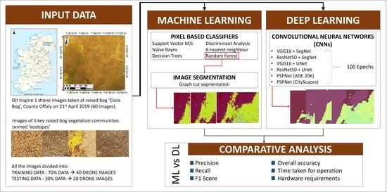
2. Study Area and Materials
3. Segmentation Using Machine Learning
3.1. Choice of the ML Classifier
3.2. Segmentation
4. Segmentation Using Deep Learning
4.1. Parameters in Convolutional Neural Network
4.1.1. Convolutional Layer
4.1.2. Pooling Layer
- Max Pooling: where the local maxima of the filtered region are carried forward.
- Average pooling: where the local average of the filtered region is carried forward.
4.1.3. Kernel Size
4.1.4. Stride
4.1.5. Padding
4.1.6. Activation Function
4.1.7. Softmax Classifier
4.1.8. Batch Normalisation
4.1.9. Additional Parameters in CNN
4.1.10. Popular CNN Models
- Stands for Visual Geometry Group
- Consists of 13 convolutional layers with three fully connected layers, hence the name VGG16.
- Each convolutional layer has kernel size = 3 with stride = 1 and padding = same.
- Each max-pooling layer has kernel = 2 and stride =2.
- Stands for Residual Network.
- A deep network, having 50 layers.
- It popularised batch normalisation.
- It uses skip connection to add information on output from a previous layer to the next layer.
4.2. CNN for Semantic Segmentation
4.2.1. Moving from a Fully Connected to a Fully Convolution Network
4.2.2. SegNet Model
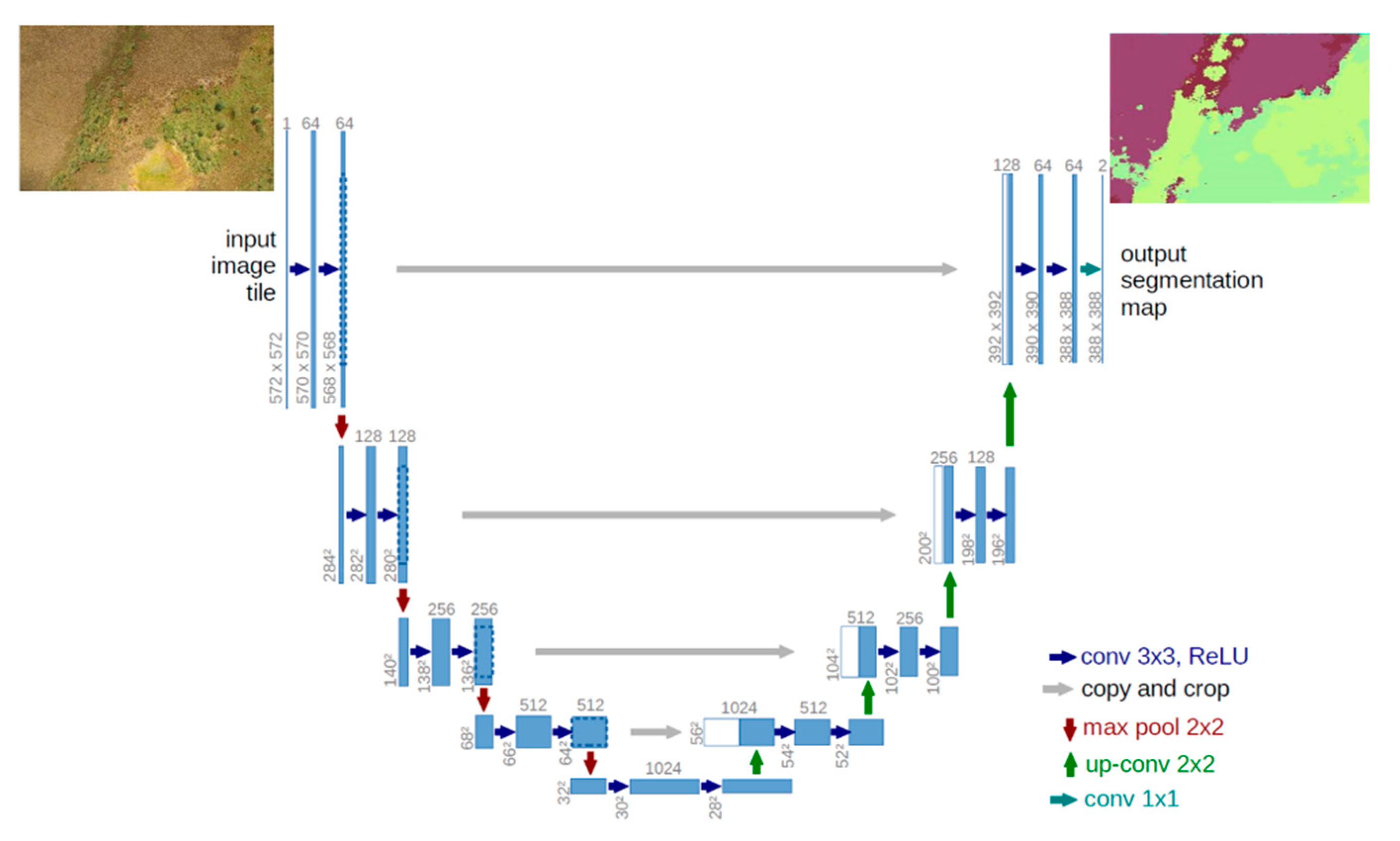
4.2.3. UNet Model
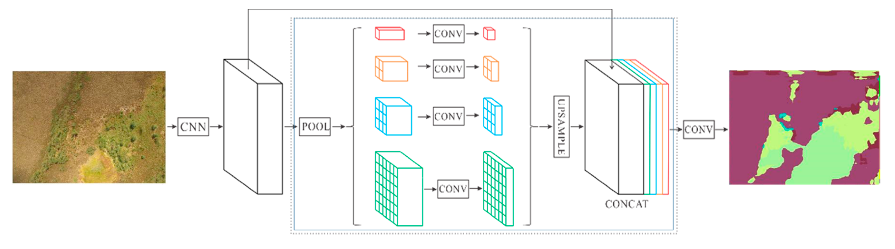
4.2.4. PSPNet Model
4.3. Methodology for the Comparison between CNN Models for the Case Study on Raised Bog Drone Images
4.3.1. Training Data Preparation
- Forty drone images were manually labelled using MATLAB-Image Labeler app [36].
- The labels (in .mat format) were converted into JPG.
- The images and labels were resized in order to use the GPU memory efficiently and to speed up the process. For resizing, the images were shrunk in the order of 2n such that the classes were clearly distinguishable. The resizing of the images was done using a bilinear interpolation technique.
- The images were resized from 3000 × 4000 to 512 × 1024 (29 × 210) for further use. The size of the image is kept rectangular in order to maintain the aspect ratio of the original drone imagery. The ratio can be decided with respect to the application. For this study, to have a fair comparison between ML and DL methods, the size of the imagery was not reduced to smaller patches.Alternatively, patches of the same size (29 × 210) can be extracted with overlapping. For this study, the small patches did not cover all the ecotopes. In a single patch, at maximum, only two ecotope classes were covered. This is due to the large size of the raised bog in the application. Therefore, to incorporate the maximum number of ecotope classes in a single image and to avoid any information loss, resizing of the images was done (instead of extracting the patches).
- After reshaping, the images were renamed such that the images and their corresponding labels can be identified.
4.3.2. Models Used for Semantic Segmentation
- VGG16 base model with SegNet architecture.
- ResNet50 base model with SegNet.
- VGG16 with UNet.
- ResNet50 with UNet
- 5.
- PspNet trained on ADE 20K dataset.
- 6.
- PspNet trained on Cityscapes dataset.
5. Results
5.1. Machine Learning
5.2. Deep Learning
6. Discussion
7. Conclusions
Author Contributions
Funding
Acknowledgments
Conflicts of Interest
References
- Bhatnagar, S.; Gill, L.; Regan, S.; Naughton, O.; Johnston, P.; Waldren, S.; Ghosh, B. Mapping Vegetation Communities Inside Wetlands Using Sentinel-2 Imagery in Ireland. Int. J. Appl. Earth Obs. Geoinf. 2020, 88, 102083. [Google Scholar] [CrossRef]
- Hirano, A.; Madden, M.; Welch, R. Hyperspectral image data for mapping wetland vegetation. Wetlands 2003, 23, 436–448. [Google Scholar] [CrossRef]
- Pengra, B.W.; Johnston, C.A.; Loveland, T.R. Mapping an invasive plant, Phragmites australis, in coastal wetlands using the EO-1 Hyperion hyperspectral sensor. Remote. Sens. Environ. 2007, 108, 74–81. [Google Scholar] [CrossRef]
- Álvarez-Taboada, F.; Araújo-Paredes, C.; Julián-Pelaz, J. Mapping of the Invasive Species Hakea sericea Using Unmanned Aerial Vehicle (UAV) and WorldView-2 Imagery and an Object-Oriented Approach. Remote. Sens. 2017, 9, 913. [Google Scholar] [CrossRef] [Green Version]
- Baena, S.; Moat, J.; Whaley, O.; Boyd, D.S. Identifying species from the air: UAVs and the very high resolution challenge for plant conservation. PLoS ONE 2017, 12, e0188714. [Google Scholar] [CrossRef] [Green Version]
- Dvořák, P.; Müllerová, J.; Bartaloš, T.; Brůna, J. Unmanned Aerial Vehicles for Alien Plant Species Detection and Monitoring. ISPRS Int. Arch. Photogramm. Remote. Sens. Spat. Inf. Sci. 2015, 40, 83–90. [Google Scholar] [CrossRef] [Green Version]
- Hill, D.; Tarasoff, C.; Whitworth, G.E.; Baron, J.; Bradshaw, J.; Church, J.S. Utility of unmanned aerial vehicles for mapping invasive plant species: A case study on yellow flag iris (Iris pseudacorus L.). Int. J. Remote. Sens. 2016, 38, 2083–2105. [Google Scholar] [CrossRef]
- Ruwaimana, M.; Satyanarayana, B.; Otero, V.; Muslim, A.M.; Muhammad, A.M.; Ibrahim, S.; Raymaekers, D.; Koedam, N.; Dahdouh-Guebas, F. The advantages of using drones over space-borne imagery in the mapping of mangrove forests. PLoS ONE 2018, 13, e0200288. [Google Scholar] [CrossRef] [Green Version]
- Chabot, D.; Dillon, C.; Shemrock, A.; Weissflog, N.; Sager, E.P.S. An Object-Based Image Analysis Workflow for Monitoring Shallow-Water Aquatic Vegetation in Multispectral Drone Imagery. ISPRS Int. J. Geo Inf. 2018, 7, 294. [Google Scholar] [CrossRef] [Green Version]
- Han, Y.-G.; Yoo, S.H.; Kwon, O. Possibility of applying unmanned aerial vehicle (UAV) and mapping software for the monitoring of waterbirds and their habitats. J. Ecol. Environ. 2017, 41, 21. [Google Scholar] [CrossRef]
- Zheng, H.; Cheng, T.; Li, D.; Zhou, X.; Yao, X.; Tian, Y.; Cao, W.; Zhu, Y. Evaluation of RGB, Color-Infrared and Multispectral Images Acquired from Unmanned Aerial Systems for the Estimation of Nitrogen Accumulation in Rice. Remote. Sens. 2018, 10, 824. [Google Scholar] [CrossRef] [Green Version]
- Govender, M.; Chetty, K.; Bulcock, H. A review of hyperspectral remote sensing and its application in vegetation and water resource studies. Water SA 2009, 33. [Google Scholar] [CrossRef] [Green Version]
- Boon, M.A.; Greenfield, R.; Tesfamichael, S. Wetland assessment using unmanned aerial vehicle (UAV) photogrammetry. Remote. Sens. Spat. Inf. Sci. 2016, XLI-B1, 781–788. [Google Scholar]
- Treboux, J.; Genoud, D. Improved Machine Learning Methodology for High Precision Agriculture. In Proceedings of the 2018 Global Internet of Things Summit (GIoTS), Bilbao, Spain, 4–7 June 2018; Institute of Electrical and Electronics Engineers (IEEE): Piscataway, NJ, USA, 2018; pp. 1–6. [Google Scholar]
- Pap, M.; Király, S.; Moljak, S. Investigating the usability of UAV obtained multispectral imagery in tree species segmentation. ISPRS Int. Arch. Photogramm. Remote. Sens. Spat. Inf. Sci. 2019, XLII-2/W18, 159–165. [Google Scholar] [CrossRef] [Green Version]
- Zuo, Z. Remote Sensing Image Extraction of Drones for Agricultural Applications. Rev. Fac. Agron. Univ. Zulia 2019, 36, 1202–1212. [Google Scholar]
- Parsons, M.; Bratanov, D.; Gaston, K.J.; Gonzalez, F. UAVs, hyperspectral remote sensing, and machine learning revolutionising reef monitoring. Sensors 2018, 18, 2026. [Google Scholar] [CrossRef] [Green Version]
- Miyamoto, H.; Momose, A.; Iwami, S. UAV image classification of a riverine landscape by using machine learning techniques. EGU Gen. Assem. Conf. Abstr. 2018, 20, 5919. [Google Scholar]
- Zimudzi, E.; Sanders, I.; Rollings, N.; Omlin, C. Segmenting mangrove ecosystems drone images using SLIC superpixels. Geocarto Int. 2018, 34, 1648–1662. [Google Scholar] [CrossRef]
- Höser, T.; Kuenzer, C. Object Detection and Image Segmentation with Deep Learning on Earth Observation Data: A Review-Part I: Evolution and Recent Trends. Remote. Sens. 2020, 12, 1667. [Google Scholar] [CrossRef]
- Lee, D.; Kim, J.; Lee, D.-W. Robust Concrete Crack Detection Using Deep Learning-Based Semantic Segmentation. Int. J. Aeronaut. Space Sci. 2019, 20, 287–299. [Google Scholar] [CrossRef]
- Zhang, C.; Wang, L.; Yang, R. Semantic segmentation of urban scenes using dense depth maps. In Proceedings of the European Conference on Computer Vision, Crete, Greece, 5–10 September 2010; Springer: Berlin/Heidelberg, Germany, 2010; pp. 708–721. [Google Scholar]
- Montoya-Zegarra, J.A.; Wegner, J.D.; Ladický, L.; Schindler, K. Semantic segmentation of aerial images in urban areas with class-specific higher-order cliques. ISPRS Ann. Photogramm. Remote. Sens. Spat. Inf. Sci. 2015, 2, 127–133. [Google Scholar] [CrossRef] [Green Version]
- Dechesne, C.; Mallet, C.; Le Bris, A.; Gouet-Brunet, V. Semantic segmentation of forest stands of pure species combining airborne lidar data and very high resolution multispectral imagery. ISPRS J. Photogramm. Remote. Sens. 2017, 126, 129–145. [Google Scholar] [CrossRef]
- Cui, B.; Zhang, Y.; Li, X.; Wu, J.; Lu, Y. WetlandNet: Semantic Segmentation for Remote Sensing Images of Coastal Wetlands via Improved UNet with Deconvolution. In Proceedings of the International Conference on Genetic and Evolutionary Computing, Qingdao, China, 1–3 November 2019; Springer: Singapore, 2019; pp. 281–292. [Google Scholar]
- Jiang, J.; Feng, X.; Liu, F.; Xu, Y.; Huang, H. Multi-Spectral RGB-NIR Image Classification Using Double-Channel CNN. IEEE Access 2019, 7, 20607–20613. [Google Scholar] [CrossRef]
- Kentsch, S.; Caceres, M.L.L.; Serrano, D.; Roure, F.; Donoso, Y.D. Computer Vision and Deep Learning Techniques for the Analysis of Drone-Acquired Forest Images, a Transfer Learning Study. Remote Sens. 2020, 12, 1287. [Google Scholar] [CrossRef] [Green Version]
- Nigam, I.; Huang, C.; Ramanan, D. Ensemble knowledge transfer for semantic segmentation. In Proceedings of the 2018 IEEE Winter Conference on Applications of Computer Vision (WACV), Lake Tahoe, NV, USA, 12–15 March 2018; Institute of Electrical and Electronics Engineers (IEEE): Piscataway, NJ, USA, 2018; pp. 1499–1508. [Google Scholar]
- Do, D.; Pham, F.; Raheja, A.; Bhandari, S. Machine learning techniques for the assessment of citrus plant health using UAV-based digital images. In Proceedings of the Autonomous Air and Ground Sensing Systems for Agricultural Optimization and Phenotyping III, Baltimore, MD, USA, 15–16 April 2019; International Society for Optics and Photonics: Bellingham, WA, USA, 2019; Volume 10664, p. 1066400. [Google Scholar]
- Bhatnagar, S.; Ghosh, B.; Regan, S.; Naughton, O.; Johnston, P.; Gill, L. Monitoring environmental supporting conditions of a raised bog using remote sensing techniques. Proc. Int. Assoc. Hydrol. Sci. 2018, 380, 9–15. [Google Scholar] [CrossRef]
- Bhatnagar, S.; Ghosh, B.; Regan, S.; Naughton, O.; Johnston, P.; Gill, L. Remote Sensing Based Ecotope Mapping and Transfer of Knowledge in Raised Bogs. Geophys. Res. Abstr. 2019, 21, 1. [Google Scholar]
- ESRI. ArcMap Desktop; (Version 10.6.1); Esri Inc.: Redlands, CA, USA, 2019. [Google Scholar]
- ESRI “World Imagery” [High Resolution 30 cm Imagery]. Scale ~1:280 (0.03 m). Available online: http://www.arcgis.com/home/item.html?id=10df2279f9684e4a9f6a7f08febac2a9 (accessed on 25 November 2019).
- Shi, J.; Malik, J. Normalised cuts and image segmentation. IEEE Trans. Pattern Anal. Mach. Intell. 2000, 22, 888–905. [Google Scholar]
- Feng, Q.; Liu, J.; Gong, J. UAV remote sensing for urban vegetation mapping using random forest and texture analysis. Remote Sens. 2015, 7, 1074–1094. [Google Scholar] [CrossRef] [Green Version]
- MATLAB; Version R2019b; The MathWorks Inc.: Natick, MA, USA, 2019.
- Tavares, J.; Jorge, R.N. Computational Vision and Medical Image Processing V. In Proceedings of the 5th Eccomas Thematic Conference on Computational Vision and Medical Image Processing, VipIMAGE 2015, Tenerife, Spain, 19–21 October 2015; CRC Press: Boca Raton, FL, USA, 2015. [Google Scholar]
- Schwenker, F.; Abbas, H.M.; El Gayar, N.; Trentin, E. Artificial Neural Networks in Pattern Recognition. In Proceedings of the 7th IAPR TC3 Workshop, ANNPR 2016, Ulm, Germany, 28–30 September 2016; Springer: New York, NY, USA, 2018. [Google Scholar]
- Chai, H.Y.; Wee, L.K.; Swee, T.T.; Hussain, S. Gray-level co-occurrence matrix bone fracture detection. WSEAS Trans. Syst. 2011, 10, 7–16. [Google Scholar] [CrossRef] [Green Version]
- Salem, Y.B.; Nasri, S. Texture classification of woven fabric based on a GLCM method and using multiclass support vector machine. In Proceedings of the 2009 6th International Multi-Conference on Systems, Signals and Devices, Jerba, Tunisia, 23–26 March 2009; Institute of Electrical and Electronics Engineers (IEEE): Piscataway, NJ, USA, 2009; pp. 1–8. [Google Scholar]
- Wu, Y.; Zhou, Y.; Saveriades, G.; Agaian, S.; Noonan, J.P.; Natarajan, P. Local Shannon entropy measure with statistical tests for image randomness. Inf. Sci. 2013, 222, 323–342. [Google Scholar] [CrossRef] [Green Version]
- Mardia, K.V. Measures of multivariate skewness and kurtosis with applications. Biometrika 1970, 57, 519–530. [Google Scholar] [CrossRef]
- Stoer, M.; Wagner, F. A simple min-cut algorithm. J. ACM 1997, 44, 585–591. [Google Scholar] [CrossRef]
- Ishida, T.; Kurihara, J.; Viray, F.A.; Namuco, S.B.; Paringit, E.C.; Perez, G.J.; Marciano, J.J.J. A novel approach for vegetation classification using UAV-based hyperspectral imaging. Comput. Electron. Agric. 2018, 144, 80–85. [Google Scholar] [CrossRef]
- Braun, A.C.; Weidner, U.; Hinz, S. Support vector machines for vegetation classification–A revision. Photogramm. Fernerkund. Geoinf. 2010, 2010, 273–281. [Google Scholar] [CrossRef]
- Laliberte, A.S.; Rango, A. Texture and scale in object-based analysis of subdecimeter resolution unmanned aerial vehicle (UAV) imagery. IEEE Trans. Geosci. Remote Sens. 2009, 47, 761–770. [Google Scholar] [CrossRef] [Green Version]
- Özlem, A. Mapping land use with using Rotation Forest algorithm from UAV images. Eur. J. Remote Sens. 2017, 50, 269–279. [Google Scholar] [CrossRef] [Green Version]
- Meng, X.; Shang, N.; Zhang, X.; Li, C.; Zhao, K.; Qiu, X.; Weeks, E. Photogrammetric UAV Mapping of Terrain under Dense Coastal Vegetation: An Object-Oriented Classification Ensemble Algorithm for Classification and Terrain Correction. Remote Sens. 2017, 9, 1187. [Google Scholar] [CrossRef] [Green Version]
- Friedl, M.A.; Brodley, C.E. Decision tree classification of land cover from remotely sensed data. Remote Sens. Environ. 1997, 61, 399–409. [Google Scholar] [CrossRef]
- Cheng, J.; Greiner, R. Comparing Bayesian network classifiers. In Proceedings of the Fifteenth conference on Uncertainty in artificial intelligence, Stockholm, Sweden, 30 July–1 August 1999; Morgan Kaufmann Publishers Inc.: Burlington, MA, USA, 1999; pp. 101–108. [Google Scholar]
- Balakrishnama, S.; Ganapathiraju, A. Linear discriminant analysis-a brief tutorial. Inst. Signal Inf. Process. 1998, 18, 1–8. [Google Scholar]
- Cortes, C.; Vapnik, V. Support vector machine. Mach. Learn. 1995, 20, 273–297. [Google Scholar] [CrossRef]
- Laaksonen, J.; Oja, E. Classification with learning k-nearest neighbors. In Proceedings of the International Conference on Neural Networks (ICNN’96), Washington, DC, USA, 3–6 June 1996; Institute of Electrical and Electronics Engineers (IEEE): Piscataway, NJ, USA, 1996; Volume 3, pp. 1480–1483. [Google Scholar]
- Liaw, A.; Wiener, M. Classification and regression by randomForest. News 2020, 2, 18–22. [Google Scholar]
- Ross, Q.J. C4. 5: Programs for Machine Learning; Morgan Kaufmann Publishers: San Mateo, CA, USA, 1993. [Google Scholar]
- Breiman, L.; Friedman, J.; Stone, C.J.; Olshen, R.A. Classification and Regression Trees; CRC Press: Boca Raton, FL, USA, 1984. [Google Scholar]
- Boykov, Y.; Kolmogorov, V. An experimental comparison of min-cut/max-flow algorithms for energy minimisation in vision. IEEE Trans. Pattern Anal. Mach. Intell. 2004, 26, 1124–1137. [Google Scholar] [CrossRef] [PubMed] [Green Version]
- MATLAB Wrapper for Graph Cut. Shai Bagon. Available online: https://github.com/shaibagon/GCMex (accessed on 12 December 2019).
- Boykov, Y.; Veksler, O.; Zabih, R. Fast approximate energy minimisation via graph cuts. IEEE Trans. Pattern Anal. Mach. Intell. 2001, 23, 1222–1239. [Google Scholar] [CrossRef] [Green Version]
- Masci, J.; Meier, U.; Ciresan, D.; Schmidhuber, J.; Fricout, G. Steel defect classification with max-pooling convolutional neural networks. In Proceedings of the 2012 International Joint Conference on Neural Networks (IJCNN), Brisbane, Australia, 10–15 June 2012; Institute of Electrical and Electronics Engineers (IEEE): Piscataway, NJ, USA, 2012; pp. 1–6. [Google Scholar]
- Li, Q.; Cai, W.; Wang, X.; Zhou, Y.; Feng, D.D.; Chen, M. Medical image classification with convolutional neural network. In Proceedings of the 2014 13th International Conference on Control Automation Robotics & Vision (ICARCV), Singapore, 10–12 December 2014; Institute of Electrical and Electronics Engineers (IEEE): Piscataway, NJ, USA, 2014; pp. 844–848. [Google Scholar]
- Sharma, S. Activation functions in neural networks. Towards Data Sci. 2017, 6, 310–316. [Google Scholar]
- Nwankpa, C.; Ijomah, W.; Gachagan, A.; Marshall, S. Activation functions: Comparison of trends in practice and research for deep learning. arXiv 2018, arXiv:1811.03378. [Google Scholar]
- Özkan, C.; Erbek, F.S. The comparison of activation functions for multispectral Landsat TM image classification. Photogramm. Eng. Remote Sens. 2003, 69, 1225–1234. [Google Scholar] [CrossRef]
- Karlik, B.; Olgac, A.V. Performance analysis of various activation functions in generalised MLP architectures of neural networks. Int. J. Artif. Intell. Expert Syst. 2011, 1, 111–122. [Google Scholar]
- Bircanoğlu, C.; Arıca, N. A comparison of activation functions in artificial neural networks. In Proceedings of the 2018 26th Signal Processing and Communications Applications Conference (SIU), Izimir, Turkey, 2–5 May 2018; Institute of Electrical and Electronics Engineers (IEEE): Piscataway, NJ, USA, 2018; pp. 1–4. [Google Scholar]
- Bottou, L. Online learning and stochastic approximations. On-line Learn. Neural Netw. 1998, 17, 142. [Google Scholar]
- Fukumizu, K. Effect of batch learning in multilayer neural networks. Gen 1998, 1, 1E–03E. [Google Scholar]
- Bottou, L. Stochastic gradient learning in neural networks. Proc. Neuro Nımes 1991, 91, 12. [Google Scholar]
- Paine, T.; Jin, H.; Yang, J.; Lin, Z.; Huang, T. Gpu asynchronous stochastic gradient descent to speed up neural network training. arXiv 2013, arXiv:1312.6186. [Google Scholar]
- Han, S.; Pool, J.; Tran, J.; Dally, W. Learning both weights and connections for efficient neural network. In Proceedings of the Advances in Neural Information Processing Systems, Montreal, QC, CA, 7–12 December 2015; Neural Information Processing Systems Foundation, Inc. (NIPS): San Diego, CA, USA, 2015; pp. 1135–1143. [Google Scholar]
- Van Den Doel, K.; Ascher, U.; Haber, E. The Lost Honour of l2-Based Regularization; (Radon Series in Computational and Applied Math); De Gruyter: Berlin, Germany, 2013. [Google Scholar]
- Atienza, R. Advanced Deep Learning with Keras: Apply Deep Learning Techniques, Autoencoders, GANs, Variational Autoencoders, Deep Reinforcement Learning, Policy Gradients, and More; Packt Publishing Ltd.: Birmingham, UK, 2018. [Google Scholar]
- Kingma, D.P.; Ba, J. Adam: A method for stochastic optimisation. arXiv 2014, arXiv:1412.6980. [Google Scholar]
- Simonyan, K.; Zisserman, A. Very deep convolutional networks for large-scale image recognition. arXiv 2014, arXiv:1409.1556. [Google Scholar]
- He, K.; Zhang, X.; Ren, S.; Sun, J. Deep residual learning for image recognition. In Proceedings of the IEEE Conference on Computer Vision and Pattern Recognition, Las Vegas, NV, USA, 27–30 June 2016; Institute of Electrical and Electronics Engineers (IEEE): Piscataway, NJ, USA, 2016; pp. 770–778. [Google Scholar]
- Cheng, K.; Cheng, X.; Wang, Y.; Bi, H.; Benfield, M.C. Enhanced convolutional neural network for plankton identification and enumeration. PLoS ONE 2019, 14, e0219570. [Google Scholar] [CrossRef] [PubMed] [Green Version]
- Qassim, H.; Verma, A.; Feinzimer, D. Compressed residual-VGG16 CNN model for big data places image recognition. In Proceedings of the 2018 IEEE 8th Annual Computing and Communication Workshop and Conference (CCWC), Las Vegas, NV, USA, 8–10 January 2018; Institute of Electrical and Electronics Engineers (IEEE): Piscataway, NJ, USA, 2018; pp. 169–175. [Google Scholar]
- Ghosh, S.; Das, N.; Das, I.; Maulik, U. Understanding deep learning techniques for image segmentation. ACM Comput. Surv. (CSUR) 2019, 52, 73. [Google Scholar] [CrossRef] [Green Version]
- Badrinarayanan, V.; Kendall, A.; Cipolla, R. Segnet: A deep convolutional encoder-decoder architecture for image segmentation. IEEE Trans. Pattern Anal. Mach. Intell. 2017, 39, 2481–2495. [Google Scholar] [CrossRef]
- Ronneberger, O.; Fischer, P.; Brox, T. U-net: Convolutional networks for biomedical image segmentation. In Proceedings of the International Conference on Medical Image Computing and Computer-Assisted Intervention, Munich, Germany, 5–9 October 2015; Springer: Cham, Switzerland, 2015; pp. 234–241. [Google Scholar]
- Zhao, H.; Shi, J.; Qi, X.; Wang, X.; Jia, J. Pyramid scene parsing network. In Proceedings of the IEEE Conference on Computer Vision and Pattern Recognition, Honolulu, HI, USA, 21–26 July 2017; Institute of Electrical and Electronics Engineers (IEEE): Piscataway, NJ, USA, 2017; pp. 2881–2890. [Google Scholar]
- He, K.; Zhang, X.; Ren, S.; Sun, J. Spatial pyramid pooling in deep convolutional networks for visual recognition. IEEE Trans. Pattern Anal. Mach. Intell. 2015, 37, 1904–1916. [Google Scholar] [CrossRef] [Green Version]
- Python Software Foundation. Python Language Reference, Version 3.7. Available online: http://www.python.org (accessed on 20 June 2020).
- Divamgupta. Image-Segmentation-Keras. 2019. Available online: https://github.com/divamgupta/image-segmentation-keras.git (accessed on 20 June 2020).
- Russakovsky, O.; Deng, J.; Su, H.; Krause, J.; Satheesh, S.; Ma, S.; Berg, A.C. Imagenet large scale visual recognition challenge. Int. J. Comput. Vis. 2015, 115, 211–252. [Google Scholar] [CrossRef] [Green Version]
- Zhou, B.; Zhao, H.; Puig, X.; Fidler, S.; Barriuso, A.; Torralba, A. Scene parsing through ade20k dataset. In Proceedings of the IEEE Conference on Computer Vision and Pattern Recognition, Honolulu, HI, USA, 21–26 July 2017; Institute of Electrical and Electronics Engineers (IEEE): Piscataway, NJ, USA, 2017; pp. 633–641. [Google Scholar]
- Cordts, M.; Omran, M.; Ramos, S.; Rehfeld, T.; Enzweiler, M.; Benenson, R.; Schiele, B. The cityscapes dataset for semantic urban scene understanding. In Proceedings of the IEEE Conference on Computer Vision and Pattern Recognition, Las Vegas, NV, USA, 27–30 June 2016; Institute of Electrical and Electronics Engineers (IEEE): Piscataway, NJ, USA, 2016; pp. 3213–3223. [Google Scholar]
- Andrews, H.C.; Patterson, C.L. Digital interpolation of discrete images. IEEE Trans. Comput. 1976, 100, 196–202. [Google Scholar] [CrossRef]
- Liu, Y.; Starzyk, J.A.; Zhu, Z. Optimised approximation algorithm in neural networks without overfitting. IEEE Trans. Neural Netw. 2008, 19, 983–995. [Google Scholar]
- Grm, K.; Štruc, V.; Artiges, A.; Caron, M.; Ekenel, H.K. Strengths and weaknesses of deep learning models for face recognition against image degradations. IET Biom. 2017, 7, 81–89. [Google Scholar] [CrossRef] [Green Version]
- Yim, J.; Joo, D.; Bae, J.; Kim, J. A gift from knowledge distillation: Fast optimisation, network minimisation and transfer learning. In Proceedings of the IEEE Conference on Computer Vision and Pattern Recognition, Honolulu, HI, USA, 21–26 July 2017; Institute of Electrical and Electronics Engineers (IEEE): Piscataway, NJ, USA, 2017; pp. 4133–4141. [Google Scholar]


| Property | Description |
|---|---|
| Contrast | Intensity difference between pixels compared to its neighbour for the whole image [37]. |
| Correlation | Correlation of a pixel and its neighbour for the whole image [38]. |
| Energy | Sum of squared elements in gray level co-occurrence matrix (GLCM) [39]. |
| Homogeneity | Closeness of the distribution of pixels in the GLCM to its diagonal [40]. |
| Mean | Mean of the area across the window |
| Variance | Variance of the area across the window |
| Entropy (e) | Statistical measure of randomness where contains the normalised histogram counts |
| Range | Range of the area across the window [41]. |
| Skewness (S) | Asymmetry of the data over the mean value [42]. S = E(p − μ)3/σ3, where µ is the mean of the pixel p, σ is the standard deviation of p, and E represents the expected value. |
| Kurtosis (K) | Distribution to be prone to outliers [42]; K = E(p − μ)4/σ4 |
| Name | Parameter | Model Accuracy | Misclassification Cost | Training Time (s) |
|---|---|---|---|---|
| Decision trees | Max. no. of splits = 20; split criterion = Gini’s diversity index | 87.4 | 736 | 7.3 |
| Discriminant analysis | Kernel = quadratic | 89.4 | 618 | 8.6 |
| Naïve Bayes | Kernel = Gaussian | 78.3 | 1271 | 19.5 |
| Support vector machine | Kernel = radial basis function (rbf) = 0.25 | 91.9 | 472 | 112.5 |
| K nearest neighbour | No. of neighbours = 2; distance = Euclidean | 91.0 | 528 | 378.8 |
| Random forest | No. of trees (t) = 100 (1000 samples with repetition); total no. of splits = 5853 | 92.9 | 454 | 59.2 |
| RGB Features | RGB + Textural Features | |
|---|---|---|
| 83.3 | 85.1 | |
| 82.9 | 84.8 |
| RF (RGB) | RF (RGB + TEXTURAL) | SEGNET + VGG16 | SEGNET + RESNET50 | |||||||||||||
| M | SMSC | C | AF | M | SMSC | C | AF | M | SMSC | C | AF | M | SMSC | C | AF | |
| M | 58,405 | 1012 | 988 | 36,321 | 59,781 | 1598 | 1002 | 38,241 | 43,872 | 8854 | 2500 | 71,005 | 62,870 | 1631 | 835 | 16,360 |
| SMSC | 734 | 155,583 | 4979 | 2033 | 600 | 188,296 | 4608 | 587 | 7952 | 122,544 | 15,691 | 9514 | 3000 | 162,651 | 3005 | 2639 |
| C | 328 | 3862 | 77,939 | 44,321 | 256 | 4150 | 83,930 | 34,658 | 2831 | 18,529 | 77,369 | 73,108 | 967 | 4895 | 98,584 | 28,330 |
| AF | 38,010 | 3211 | 43,509 | 142,707 | 39,023 | 3079 | 32,584 | 112,589 | 65,896 | 21,251 | 64,211 | 99,833 | 18,470 | 14,110 | 10,358 | 148,383 |
| Precision | 0.59 | 0.94 | 0.61 | 0.62 | 0.59 | 0.96 | 0.68 | 0.66 | 0.35 | 0.79 | 0.45 | 0.40 | 0.77 | 0.95 | 0.74 | 0.78 |
| Recall | 0.60 | 0.95 | 0.61 | 0.63 | 0.60 | 0.95 | 0.69 | 0.66 | 0.36 | 0.72 | 0.48 | 0.39 | 0.74 | 0.89 | 0.87 | 0.76 |
| F1 score | 0.60 | 0.94 | 0.61 | 0.62 | 0.60 | 0.95 | 0.68 | 0.66 | 0.36 | 0.75 | 0.47 | 0.40 | 0.75 | 0.92 | 0.80 | 0.77 |
| UNET + VGG16 | UNET + RESENET50 | PSPNET ADE20K | PSPNET CITYSCAPES | |||||||||||||
| M | SMSC | C | AF | M | SMSC | C | AF | M | SMSC | C | AF | M | SMSC | C | AF | |
| M | 82,589 | 9510 | 3258 | 36,951 | 73,897 | 1008 | 258 | 3371 | 36,351 | 9822 | 631 | 5311 | 128,890 | 78,353 | 36,118 | 63,001 |
| SMSC | 10,254 | 146,933 | 9800 | 19,759 | 4096 | 152,363 | 3690 | 15,892 | 15,200 | 210,052 | 6323 | 28,200 | 73,570 | 107,781 | 2988 | 4820 |
| C | 4523 | 12,967 | 96,582 | 35,489 | 982 | 5183 | 90,258 | 28,105 | 987 | 7921 | 96,587 | 3715 | 38,562 | 5815 | 32,510 | 12,377 |
| AF | 32,563 | 19,638 | 34,822 | 83,417 | 5101 | 14,852 | 22,110 | 155,446 | 3074 | 21,520 | 5300 | 127,296 | 58,360 | 7826 | 13,524 | 57,450 |
| Precision | 0.62 | 0.79 | 0.65 | 0.49 | 0.94 | 0.87 | 0.72 | 0.79 | 0.70 | 0.81 | 0.88 | 0.81 | 0.42 | 0.57 | 0.36 | 0.42 |
| Recall | 0.64 | 0.78 | 0.65 | 0.47 | 0.88 | 0.88 | 0.78 | 0.77 | 0.65 | 0.84 | 0.89 | 0.77 | 0.43 | 0.54 | 0.38 | 0.42 |
| F1 score | 0.63 | 0.78 | 0.66 | 0.48 | 0.91 | 0.87 | 0.75 | 0.78 | 0.67 | 0.83 | 0.89 | 0.79 | 0.43 | 0.55 | 0.37 | 0.42 |
| Pros | Cons |
|---|---|
| MACHINE LEARNING ALGORITHMS | |
|
|
| DEEP LEARNING ALGORITHMS | |
|
|
© 2020 by the authors. Licensee MDPI, Basel, Switzerland. This article is an open access article distributed under the terms and conditions of the Creative Commons Attribution (CC BY) license (http://creativecommons.org/licenses/by/4.0/).
Share and Cite
Bhatnagar, S.; Gill, L.; Ghosh, B. Drone Image Segmentation Using Machine and Deep Learning for Mapping Raised Bog Vegetation Communities. Remote Sens. 2020, 12, 2602. https://doi.org/10.3390/rs12162602
Bhatnagar S, Gill L, Ghosh B. Drone Image Segmentation Using Machine and Deep Learning for Mapping Raised Bog Vegetation Communities. Remote Sensing. 2020; 12(16):2602. https://doi.org/10.3390/rs12162602
Chicago/Turabian StyleBhatnagar, Saheba, Laurence Gill, and Bidisha Ghosh. 2020. "Drone Image Segmentation Using Machine and Deep Learning for Mapping Raised Bog Vegetation Communities" Remote Sensing 12, no. 16: 2602. https://doi.org/10.3390/rs12162602