Single-Look SAR Tomography of Urban Areas

Abstract

Synthetic aperture radar (SAR) tomography (TomoSAR) is a multibaseline interferometric technique that estimates the power spectrum pattern (PSP) along the perpendicular to the line-of-sight (PLOS) direction. TomoSAR achieves the separation of individual scatterers in layover areas, allowing for the 3D representation of urban zones. These scenes are typically characterized by buildings of different heights, with layover between the facades of the higher structures, the rooftop of the smaller edifices and the ground surface. Multilooking, as required by most spectral estimation techniques, reduces the azimuth-range spatial resolution, since it is accomplished through the averaging of adjacent values, e.g., via Boxcar filtering. Consequently, with the aim of avoiding the spatial mixture of sources due to multilooking, this article proposes a novel methodology to perform single-look TomoSAR over urban areas. First, a robust version of Capon is applied to focus the TomoSAR data, being robust against the rank-deficiencies of the data covariance matrices. Afterward, the recovered PSP is refined using statistical regularization, attaining resolution enhancement, suppression of artifacts and reduction of the ambiguity levels. The capabilities of the proposed methodology are demonstrated by means of strip-map airborne data of the Jet Propulsion Laboratory (JPL) and the National Aeronautics and Space Administration (NASA), acquired by the uninhabited aerial vehicle SAR (UAVSAR) system over the urban area of Munich, Germany in 2015. Making use of multipolarization data [horizontal/horizontal (HH), horizontal/vertical (HV) and vertical/vertical (VV)], a comparative analysis against popular focusing techniques for urban monitoring (i.e., matched filtering, Capon and compressive sensing (CS)) is addressed.

1. Introduction

Synthetic aperture radar (SAR) tomography (TomoSAR) is a multibaseline interferometric technique, whose main goal is the estimation of the power spectrum pattern (PSP) along the perpendicular to the line-of-sight (PLOS) direction [1,2]. The attainable PLOS resolution, after matched filtering, is inversely proportional to the synthesized tomographic aperture, limited at best to the Rayleigh resolution [1,3] when the spatial baselines are evenly distributed. However, the acquisition constellation must gather a sufficiently large amount of passes to prevent aliasing within the height range of interest.

In practical scenarios, the number of passes is constrained to the revisit time that leads to temporal decorrelation issues and to the viability of the individual missions to perform the numerous tracks, which translates into a limited (reduced) resolution. Furthermore, nonuniformly distributed baselines entail high sidelobes.

Consequently, in order to reach finer resolution and lower ambiguity levels, different spectral analysis inspired techniques, within the direction-of-arrival (DOA) estimation framework [2,4,5], are treated. Among the most reliable TomoSAR focusing methods there is Capon beamforming [5], well known for having better resolution and interference rejection capabilities with respect to matched filtering. Nevertheless, Capon has two important downsides, related to the inversions of the data covariance matrices that it involves. On one hand, radiometric accuracy is not preserved; on the other hand, multilooking is required to avoid the rank deficiencies of the data covariance matrices.

Capon implicitly assumes the use of well-posed (invertible) data covariance matrices. In this way, it assures having enough information to retrieve a solution that correctly suits the considered signal model [5]. Otherwise, estimating the parameters that describe the signal model (i.e., the PSP) becomes unfeasible.

Full-rank invertible data covariance matrices are constructed through multilooking, which refers to the averaging of independent realizations (looks) of the data acquisitions. However, in practice, TomoSAR is customarily treated as an ergodic process, meaning that its statistical properties are deduced from a single random realization. Thus, normally, multilooking is accomplished instead through the averaging of adjacent values among the set of data covariance matrices, e.g., via Boxcar filtering. This causes the spatial mixture of sources.

Urban scenes are typically characterized by buildings of different heights, with layover between the facades of the higher structures, the rooftop of the smaller edifices and the ground surface [6], inferring the presence of a dominant scattering mechanism per resolution cell. In contrast to many natural surfaces like glaciers and forests, urban scenarios entail the presence of fine structures; therefore, the preservation of high spatial resolution is required.

TomoSAR achieves the separation of individual scatterers in layover areas, allowing for the 3D representation of urban zones. Yet, applying Capon beamforming for focusing implicates multilooking on the set of data covariance matrices, which reduces the azimuth-range spatial resolution. An alternative for TomoSAR focusing is the usage of compressive sensing (CS) [7,8,9,10,11]. This technique permits decreasing the number of processed looks to preserve the spatial details in the azimuth-range grid.

Former studies [7,8,9] have demonstrated the remarkable capabilities of CS for urban monitoring, which include attaining super-resolution in elevation and preserving high azimuth-range spatial resolution by avoiding multilooking. For these reasons, CS has been the method of choice for urban scenarios; nonetheless, it has the main drawback of being computationally expensive. Normally, the involved convex optimization problem is not solved analytically; instead, general convex optimization algorithms are treated, which require numerous iterations to find a solution. As a result, the absence of specifically adapted efficient convex optimization algorithms makes CS computationally expensive [10,11]. Furthermore, CS tends to retrieve high ambiguity levels when the method’s parameters are not properly set.

Recent related studies [12,13,14] have demonstrated that employing statistical regularization to solve the TomoSAR inverse problem results in attaining finer resolution, reduced ambiguity levels and suppression of artifacts, incurring less computation time in contrast to CS. Particularly, we refer to two super-resolved techniques: the maximum-likelihood (ML)-based adaptive robust iterative approach (MARIA) [12,14], and the weighted covariance fitting (WCF)-inspired spectral estimator (WISE) [12].

MARIA and WISE require a priori information, expressed in the form of a first estimate of the PSP. Their performance depends on the accuracy of this first approximation. The implementation of these techniques, introduced in [12], involves the use of Capon beamforming to retrieve such a first estimate, which serves as first input (zero-step iteration) to the corresponding iterative procedures. The latter entails the mixture of sources as a consequence of spatial multilooking, since Capon requires guaranteeing the data covariance matrices to be invertible.

Taking all these matters into consideration, this article proposes a novel methodology to decrease considerably the number of processed looks necessary to perform focusing of the TomoSAR data, preserving all the advantages that the usage of statistical regularization offers.

First, we suggest utilizing a robust version of Capon beamforming, being robust against the rank deficiencies of the data covariance matrices. In this way, we achieve enhanced resolution with a reduced number of looks or even without multilooking. In this scenario, multilooking is required only to handle the multiple nondeterministic sources and in order to increase accuracy in presence of signal-dependent (multiplicative) noise [2], but not to guarantee that the data covariance matrices are invertible.

In the literature [15,16,17], we identify three robust versions of Capon, namely, robust Capon beamforming (RCB), norm-constrained Capon beamforming (NCCB) and doubly constrained robust Capon beamforming (DCRCB). According to the previous studies [15,16,17], the three techniques present similar accuracy when retrieving the local maxima locations, with RCB recovering more precise power estimations and with DCRCB having better array output interference rejection.

After applying one of these techniques, the recovered PSP is to be refined using statistical regularization. We make use of the abovementioned MARIA and WISE approaches, which perform regularization in the context of ML and WCF, respectively, but using now a robust version of Capon beamforming to provide them with a first estimation (zero-step iteration) of the PSP.

Both MARIA and WISE present similar advantages. The main difference is that WISE is more flexible to the assumed probability density function (pdf) of the observed data [12]; in contrast, MARIA assumes a Gaussian pdf [12,14]. Consequently, taking into account the a priori knowledge about the pdf of the observed data, the most suitable technique is to be chosen.

The proposed methodology is summarized in Figure 1. For demonstration purposes, in this article, we select DCRCB, which retrieves accurate signal estimates with reduced array output interference [16], and WISE [12], since we assume no a priori information about the pdf of the observed data. The reader, however, can easily adapt the proposed methodology to its convenience.

The suggested strategy is intended to deal with only one of the stated downsides of Capon beamforming: the need of multilooking to become applicable. Keep in mind that radiometric accuracy is not preserved, since the related statistical regularization techniques are iterative and involve numerous matrix inversions, along with other matrix/vector operations, to accomplish super-resolution.

Also, in this paper, the proposed methodology is pushed to its limits by taking into account the single-look case to perform TomoSAR focusing. Apart of preserving the range/azimuth spatial resolution, this set-up is useful for the study of the several point-type targets, situated in urban scenes, whose behavior tends to be deterministic. This eases the search for stable scatterers, necessary to perform persistent scatterer interferometry (PSI) [6].

Finally, the capabilities of the proposed methodology are validated by means of strip-map airborne data acquired by the uninhabited aerial vehicle SAR (UAVSAR) system of the Jet Propulsion Laboratory (JPL) and the National Aeronautics and Space Administration (NASA), over the urban area of Munich, Germany in 2015 [18]. Making use of multipolarization data [horizontal/horizontal (HH), horizontal/vertical (HV) and vertical/vertical (VV)], a comparative analysis against the aforementioned focusing techniques for urban monitoring (i.e., matched filtering, Capon and CS) is addressed. We refer first to the multilooking case in order to observe the spatial mixture of sources; later on, the single-look case is treated.

The rest of the paper is organized in the following manner: the TomoSAR signal model is reviewed in Section 2; Section 3 studies a modified version of the WISE iterative statistical regularization approach, using DCRCB to retrieve its first input (zero-step iteration); Section 4 is dedicated to present the experimental results, performed using strip-map airborne UAVSAR data; lastly, Section 5 presents a discussion on the previously given experimental results, providing also the concluding remarks.

2. TomoSAR Signal Model

Within the framework of DOA estimation, as in the previous related studies [12,13,14], the considered TomoSAR signal model is defined by the linear equation of observation (EO)

$${\left[\begin{array}{c}\begin{array}{c}\begin{array}{c} \\ y\end{array}\\ \end{array}\end{array}\right]}_{L\times 1}={\left[\begin{array}{cc} & \begin{array}{ccc} & & \begin{array}{cc} & \end{array}\end{array}\\ \begin{array}{c} \\ \end{array}& \begin{array}{c}\begin{array}{ccc} & A& \begin{array}{cc} & \end{array}\end{array}\\ \begin{array}{ccc} & & \begin{array}{cc} & \end{array}\end{array}\end{array}\end{array}\right]}_{L\times M}{\left[\begin{array}{c}\begin{array}{c}\begin{array}{c} \\ \end{array} \\ s\\ \begin{array}{c} \\ \end{array}\end{array}\end{array}\right]}_{M\times 1}+{\left[\begin{array}{c}\begin{array}{c}\begin{array}{c} \\ n\end{array}\\ \end{array}\end{array}\right]}_{L\times 1}.$$

(1)

For a certain acquisition constellation, composed of $L$ passes, the data signal vector $y$ denotes the set of focused signals for a given azimuth-range location. We assume co-registration independent on height. Vector $s$ is composed of $M$ samples, taken at the elevation positions ${\left\{z_m\right\}}_{m=1}^M$ displaced along the PLOS direction. These samples describe the continuous complex random reflectivity for a specified azimuth-range position within the illuminated scene. The $L\times M$ steering matrix $A$ is the signal formation operator (SFO) that maps the source Hilbert signal space $S$ onto the observation Hilbert signal space $Y$. Vector $n$ accounts for the additive noise.

Matrix $A$ gathers the steering vectors ${\left\{a_m\right\}}_{m=1}^M$, each one of dimension $L$, which contain the interferometric phase information associated to a source located at the PLOS elevation position ${\left\{z_m\right\}}_{m=1}^M$, above the reference focusing plane. For a given elevation position $z_m$, the corresponding steering vector is given by [4],

$$a\left(z_m\right)={\left[\begin{array}{ccc}1& \exp \left\{\mathrm{j}{k}_z{}_2{z}_m\right\}& \begin{array}{cc}\cdots & \exp \left\{\mathrm{j}{k}_z{}_L{z}_m\right\}\end{array}\end{array}\right]}^{\mathrm{T}},$$

(2)

in which

$${\left\{k_z{}_l=\left(\frac{4\pi }{\lambda }\right)\left(\frac{d_l}{r_1\sin \theta }\right)\right\}}_{l=2}^L$$

(3)

is the two-way vertical wavenumber between the master track and the $l$-th slave track. Here, ${\left\{d_l\right\}}_{l=2}^L$ is the PLOS-oriented baseline distance between the master track and the $l$-th slave track, $r_1$ is the slant-range distance to the target of interest, $\theta$ stands for the incidence angle and $\lambda$ is the carrier wavelength.

A problem is said to be well-posed in the Hadamard sense if three conditions are accomplished [19]: (i) a solution exists, (ii) the solution is unique and (iii) the solution depends continuously on the data. The TomoSAR problem is considered ill-conditioned in the Hadamard sense, since, generally, the linear EO in (1) has infinite solutions. The number of passes $L$ is normally (much) lower than the number of samples $M$, meaning that there are more unknowns $M$ than equations $L$ in (1). Moreover, the presence of additive and multiplicative noise adds statistical uncertainty to the problem. Thus, in order to guarantee well-conditioned solutions in the Hadamard sense, some constraints must be imposed to the solver to the EO in (1).

The complex random Gaussian zero-mean vectors $s$, $n$ and $y$ are characterized by their corresponding correlation matrices

$$R_s=E\left\{s{s}^{+}\right\}=D\left(b\right)=\mathrm{diag}\left(b\right),$$

(4)

$$R_n=E\left\{n{n}^{+}\right\}=N_{0}I,$$

(5)

$$R_y=E\left\{y{y}^{+}\right\}=A{R}_s{A}^{+}+R_n,$$

(6)

where ${}^{+}$ stands for the Hermitian conjugate, $E\{·\}$ is the expectation operator and factor $N_0$ is the power spectral density of the white noise power [2].

The entries of vector s are assumed to be uncorrelated. This simplifies the mathematical developments that factor into the chosen (WISE) statistical regularization approach [12], presented afterward. Therefore, we refer to the same model, with the correlation matrix $R_s$ as a diagonal matrix. Vector $b$, at the principal diagonal of the diagonal matrix $D\left(b\right)$, defines the second-order statistics of the complex reflectivity vector $s$, the backscattering power, which we refer to as the PSP.

The TomoSAR problem consists then of estimating the PSP vector $b$. For such a purpose, the different techniques within the DOA framework make use of the SFO (steering matrix) $A$ and some a priori information about the statistics of the signal and noise.

3. Single-Look TomoSAR

3.1. First Step: DCRCB

We start by briefly reviewing the Capon beamforming technique, which refers to the solution to the spatial filter design problem [5]

$${\left\{{\widehat{h}}_m=\begin{array}{c}\mathrm{argmin}\\ h_m\end{array}\left\{h_m^{+}{R}_y^{-1}{h}_m\right\}\mathrm{s}.\mathrm{t}.h_m^{+}{a}_m=1\right\}}_{m=1}^M,$$

(7)

given by

$${\left\{{\widehat{h}}_m=\frac{R_y^{-1}{a}_m}{a_m^{+}{R}_y^{-1}{a}_m}\right\}}_{m=1}^M.$$

(8)

Let us consider that $R_y$ equals the sample covariance matrix

$$Y=\frac{1}{J}{\displaystyle \sum }_{\begin{array}{c}j=1\\ \end{array}}^J{y}_{\left(j\right)}{y}_{\left(j\right)}^{+},$$

(9)

in which $J$ indicates the number of looks. Then, the power of the filter output is obtained via ${\left\{{\widehat{b}}_m={\widehat{h}}_m^{+}Y{\widehat{h}}_m\right\}}_{m=1}^M$, yielding the celebrated Capon solver

$${\left\{{\widehat{b}}_{{\mathrm{Capon}}_m}=\frac{1}{a_m^{+}{Y}^{-1}{a}_m}\right\}}_{m=1}^M.$$

(10)

There is an implicit assumption that $R_y^{-1}$ and $Y^{-1}$ exists in both (8) and (10), respectively. This assumption sets a limit ($J\ge L$) on the minimum number of independent realizations (looks) for $Y$ in (9), as $\mathrm{rank}\left(Y\right)\le L$. Note that we presume no multicollinearity when $J=L$, this is not always the case. Each matrix ${\left\{Y_{\left(j\right)}\right\}}_{\begin{array}{c}j=1\\ \end{array}}^J$ in (9), having rank one, contributes through its summation to the assembly of a full-rank matrix $Y$, constructed from $L$ linearly independent observations.

Diagonal loading [17] is a popular approach to improve the robustness of Capon against the rank-deficiencies of the data covariance matrix $Y$. However, the exact amount of diagonal loading is difficult to determine. The robust versions of Capon introduced in [15,16,17] (e.g., DCRCB), accurately calculate the amount of diagonal loading based on the uncertainty set of the steering vectors.

Generally, the modelled data correlation matrix $R_y$ in (6) does not equal the sample data covariance matrix $Y$, as assumed by Capon. The difference between $Y$ and the diagonal-loaded (thus invertible) matrix $R_y$ can be interpreted as due to steering vector errors. These steering vector errors occur normally because of the discrepancies between the assumed signal’s DOA and the true one, or due to calibration errors, when there are discrepancies between the expected array response and the actual array response.

The DCRCB technique reduces such steering vector errors by providing an approximate solution to the following minimization problem

$${\left\{{\widehat{a}}_m=\underset{a_m}{\mathrm{argmin}}\left\{a_m^{+}{R}_y^{-1}{a}_m\right\}\mathrm{s}.\mathrm{t}.{\Vert a_m-{\overline{a}}_m\Vert }^2\le \epsilon \mathrm{with}{\Vert a_m\Vert }^2=L\right\}}_{m=1}^M.$$

(11)

Consider that ${\left\{{\overline{a}}_m\right\}}_{m=1}^M$ are the correct steering vectors of the signal-of-interest. Then, assume that the steering vectors ${\left\{a_m\right\}}_{m=1}^M$ belong to the uncertainty sphere ${\{{\Vert a_m-{\overline{a}}_m\Vert }^2\le \epsilon \}}_{m=1}^M$, where $\Vert ·\Vert$ accounts for the Euclidean norm and with $\epsilon$ as a user specified parameter (degree-of-freedom).

After solving (11), the DCRCB approach is inferred from the Capon’s expression in (10), but using instead the previously computed steering vectors ${\left\{{\widehat{a}}_m\right\}}_{m=1}^M$ and the modelled data correlation matrix $R_y$ in (6). The DCRCB solver is explicitly defined through the eigen-decomposition $Y=U\Gamma U^{+}$ via (the derivation of (12) is detailed in [16])

$${\left\{{\widehat{b}}_{\mathrm{DCRCB}}=\frac{1}{\left(L-\frac{\epsilon }{2}\right)}\frac{{\left(a_m^{+}U{\left(I+{\vartheta }_m\Gamma \right)}^{-1}\Gamma U^{+}{a}_m\right)}^2}{a_m^{+}U{\left(I+{\vartheta }_m\Gamma \right)}^{-2}\Gamma U^{+}{a}_m}\right\}}_{m=1}^M,$$

(12)

where the columns of $U$ contain the eigenvectors of $Y$, and the main diagonal of the diagonal matrix $\Gamma$ gathers the respective eigenvalues ${\left\{{\mu }_l\right\}}_{l=1}^L$. Factors ${\left\{{\vartheta }_m\right\}}_{m=1}^M$ correspond to the set of Lagrange multipliers obtained from

$${\left\{\frac{{{\displaystyle \sum }}_{l=1}^L\frac{{\left|g_l\right|}^2}{\left(1/{\mu }_l+{\vartheta }_m\right)}}{{\left({{\displaystyle \sum }}_{l=1}^L\frac{{\left|g_l\right|}^2}{\left(1/{\mu }_l+{\vartheta }_m\right)}\right)}^2}=\rho \right\}}_{m=1}^M,$$

(13)

with ${\left\{g_m=U^{+}{a}_m\right\}}_{m=1}^M$ and $\rho =L/{\left(L-\epsilon /2\right)}^2$.

3.2. Second Step: WISE

The WCF minimization problem is defined by [20,21]

$${\widehat{b}}_{\mathrm{WCF}}=\underset{b}{\mathrm{argmin}}\left\{y^{+}{R}_y^{-1}y+\frac{\mathrm{tr}\left\{R_y\right\}}{\mathrm{tr}\left\{Y\right\}}\right\},$$

(14)

with $R_y=R_y\left(b\right)=AD\left(b\right)A^{+}+N_{0}I$. Here, operator $\mathrm{tr}\{·\}$ retrieves the trace of the embraced matrix.

WISE provides an approximate solution to (14), given by (the derivation of (15) is detailed in [12])

$${\left\{{\widehat{b}}_{{\mathrm{WISE}}_m}=\mathrm{tr}\left\{Y\right\}\frac{{\widehat{a}}_m^{+}{R}_y^{-1}Y{R}_y^{-1}{\widehat{a}}_m}{{\widehat{a}}_m^{+}{\widehat{a}}_m}{\widehat{b}}_m^{\left[0\right]}\right\}}_{m=1}^M.$$

(15)

Notice that WISE is solution-dependent, since it requires of a first estimate of the PSP ${\widehat{b}}^{\left[0\right]}$ as input and in order to construct the correlation matrix $R_y$ in (6).

Different initial estimates ${\widehat{b}}^{\left[0\right]}$ in (15) may produce different WCF solutions; therefore, seeking convergence, WISE is implemented in an iterative fashion [12]. Nevertheless, this only alleviates the issue to a certain extent, when the discrepancies between the different estimates ${\widehat{b}}^{\left[0\right]}$ are not highly significant. Moreover, the degradation or improvement of the retrieved solution ${\widehat{b}}_{\mathrm{WISE}}$ still depends on the accuracy of the first estimate ${\widehat{b}}^{\left[0\right]}$.

As depicted in Algorithm 1, WISE refines a first estimate of the PSP after each iteration ${\{{\widehat{b}}^{\left[i\right]}\}}_{i=0}^I$ until achieving convergence ${\widehat{b}}^{\left[i=I\right]}$. In practice, the iterative process is finished either by reaching a user tolerance control level ${\epsilon }_{TL}$ or a maximum number of iterations $i_{\mathrm{MAX}}$. This article suggests retrieving the first estimate ${\widehat{b}}^{\left[0\right]}$ in (15) using DCRCB [15,16]. Being a refined robust version of Capon beamforming, DCRCB permits reducing the number of looks significantly, being applicable even for the single-look case. The algorithm in Algorithm 1 has the same structure as in [12], the main change is the replacement of Capon by DCRCB, employed to recover the first input ${\widehat{b}}^{\left[0\right]}={\widehat{b}}_{\mathrm{DCRCB}}$.

Algorithm 1. Modified iterative implementation of WISE.

$i=0$

${\widehat{b}}^{\left[i\right]}={\widehat{b}}_{\mathrm{DCRCB}}$

do

$R_y^{-1}={(AD({\widehat{b}}^{\left[i\right]})A^{+}+N_{0}I)}^{-1}$

for $m=1,\dots ,M$

${\widehat{b}}_{{\mathrm{WISE}}_m}^{\left[i+1\right]}={\mathcal{P}}_{+\gamma }\left\{\mathrm{tr}\left\{Y\right\}\frac{{\widehat{a}}_m^{+}{R}_y^{-1}Y{R}_y^{-1}{\widehat{a}}_m}{{\widehat{a}}_m^{+}{\widehat{a}}_m}{\widehat{b}}_m^{\left[i\right]}\right\}$

$i++$

while$\Vert {\widehat{b}}^{\left[i+1\right]}-{\widehat{b}}^{\left[i\right]}\Vert >{\epsilon }_{TL}$or$i\ne i_{\mathrm{MAX}}$

$\widehat{b}={\widehat{b}}^{\left[i=I\right]}$

The projector onto convex solution sets

$${\mathcal{P}}_{+\gamma }\left\{x\right\}=\{\begin{array}{c}0,x<\gamma \\ x,x\ge \gamma \end{array}$$

(16)

is integrated into the iterative solver in order to guarantee convergence [22,23]. The minimization problem to be solved is convex, thus, it converges under the conditions that ${\{{\widehat{b}}_m^{\left[i\right]}>0\}}_{m=1}^M$ and that $R_y$ remains positive definite, as the number of iterations increases.

Consistent with the methodology presented in Figure 1, the algorithm in Algorithm 1 allows for the usage of different techniques to obtain the first input, e.g., RCB, NCCB and DCRCB [15,16,17]. On the other hand, MARIA has the exact same structure as in Algorithm 1, but using a different solver [12]

$${\hat{b}}_{{\mathrm{MARIA}}_m}^{\left[i+1\right]}={\mathcal{P}}_{+\gamma }\left\{\frac{{\widehat{a}}_m^{+}{R}_y^{-1}Y{R}_y^{-1}{\widehat{a}}_m}{{\widehat{a}}_m^{+}{R}_y^{-1}{\widehat{a}}_m}{\widehat{b}}_m^{\left[i\right]}\right\},$$

(17)

rather than ${\widehat{b}}_{{\mathrm{WISE}}_m}^{\left[i+1\right]}$. Note that the previous warnings about the TomoSAR problem being ill-conditioned do not apply, since the whole purpose of the addressed regularization techniques is to cure that same ill-conditioning.

4. Experimental Results

Due to strictly regulated air traffic, the experiments conducted in urban areas primarily use space-borne data sets rather than air-borne data acquisitions. However, the high flight altitude of the UAVSAR system of the JPL/NASA eases this constraint. In 2015 UAVSAR was flown in order to acquire L-band fully polarimetric TomoSAR data collections from Munich [18], the third largest city in Germany. Figure 2 shows one single-look-complex (SLC) image out of the stack; the presence of radio frequency interference is due to the several external sources, by instance, those coming from the Munich’s airport.

The utilized gulfstream G-III aircraft flew at a nominal altitude of 12.5 km with a swath of 22 km and length of 60 km. The incidence angles range from 25° to 65°. For the specified microwave frequency band, with 0.24 m wavelength and 80 MHz chirp bandwidth, the resultant SLC imagery has a resolution of 1.66 m in range and 0.8 m in azimuth. The TomoSAR acquisition geometry consists of seven tracks at different altitudes, as specified in

Table 1. TomoSAR acquisition geometry.

Track	Flight Altitude [m]
1	12500
2	12500 + 30
3	12500 + 90
4	12500 + 160
5	12500 + 240
6	12500 + 400
7	12500 + 600

. These were completed on a heading of 193°.

The employed $k_z$ values were chosen with the aim of attaining finer vertical resolution in such an urban environment; until now, the largest flown by the UAVSAR system for TomoSAR data acquisitions. Figure 3 shows the vertical wavenumber $k_z$ against incidence angle for the different baselines within the previously specified acquisition geometry.

Figure 4 depicts the projected impulse response, after Fourier beamforming, as a function of the incidence angle.

The expected vertical resolution $\rho =\left(\lambda r_1/2D_{{\mathrm{Tomo}}_{\mathrm{PLOS}}}\right)·\sin \left(\theta \right)$ is of about 2.8 m in the near range and of about 6 m in the far range; where $r_1=\raisebox{1ex}{$h_0$}\!\left/ \!\raisebox{-1ex}{$\cos \left(\theta \right)$}\right.$, $D_{{\mathrm{Tomo}}_{\mathrm{PLOS}}}=D_{\mathrm{Tomo}}·\sin \left(\theta \right)$, with $h_0=12800$ m as the average flight altitude and $D_{\mathrm{Tomo}}=600$ m as the vertical tomographic aperture (see Table 1).

Before using the suggested methodology (as in Figure 1) to perform TomoSAR, we first define the region-of-interest (ROI), where the edifice of the Bavarian state chancellery is located. Figure 5 shows the respective intensity images, with respect to the master track, for all polarizations (HH, HV and VV). The azimuth and range indices are displayed, acting as a guide to identify the azimuth and range bounds of the ROI, which is specified through a red rectangle. The tomograms presented afterward correspond to the lines crossing the ROI, spanning about 194 m along azimuth with a 1.2° slope.

The tomographic slices correspond to the edifice of the Bavarian state chancellery, denoted in Figure 6a–c through a blue rectangle and a yellow dashed (half) circle. Figure 6a shows the Google Earth© image of the test region, whereas Figure 5b shows the respective polarimetric SLC SAR image [the colors correspond to the channels HH (red), VV (blue) and HV (green)]. As it can be observed in Figure 6c, the edifice of the Bavarian state chancellery comprises two wings (22 m high) and a central building (28 m high), the latter with two upper floors and a dome on top (52 m high at its peak). Both wings have a ceiling made of glass. The area depicted via the blue rectangle in Figure 6a–c includes the two wings and the central building of the edifice aforementioned, whereas the yellow dashed (half) circle in Figure 6a–c encloses the dome.

We start by considering the multilooking case, performing Boxcar filtering on the set of data covariance matrices using a 15 × 3 (range/azimuth) pixel window. More pixels in range are employed for multilooking, in order to make more evident the spatial mixture of sources when comparing to the single-look case, presented later on. One of the main challenges in SAR remote sensing for urban areas is related to the presence of several scattering mechanisms concurring in the backscattered signal. In this context, a study carried in [24], exploiting coherent scatterers, has shown that a data-driven approach can partially help in reconstructing the orientation/radiation pattern of scatterers. Generally, complex scatterers like buildings are randomly oriented w.r.t. the SAR coordinates and one cannot assume their orientation being favorable to the flight direction. Therefore, due to the required multilooking, scattering contribution (source) mixtures will be recorded in the covariance matrix impacting the final reconstruction. For this reason, although the considered building is by chance parallel to the azimuth/flight direction, range multilooking has also been included. This is also to show that, the methodology presented in this article, which drastically reduces the need for looks, has also the advantage to present a lower sensitivity to the source mixtures/building orientation.

As a reference, we first apply matched spatial filtering (MSF) [13], on the sample covariance matrices, to focus the multilooked TomoSAR data. Subsequently, we refer to the area depicted via the red line in Figure 5, crossing the ROI. It can be seen in Figure 7a, that the two wings, constituting the considered edifice (enclosed by the blue rectangle in Figure 6), are more noticeable for the HH and VV polarizations. The central building and the dome (encircled by the yellow dashed line in Figure 6) can be distinguished in all polarizations, with HV offering additional information. Nonetheless, the presence of artifacts and high ambiguity levels hamper the interpretation of the results obtained by MSF. In order to avoid these issues, more sophisticated approaches are normally utilized, which attain enhanced resolution too.

Next, for comparison purposes, we refer also to some of the most popular competing state-of-the-art nonparametric TomoSAR focusing techniques, namely, Capon [5], DCRCB [15,16] and CS [10,11]. Next, we apply WISE as in [12], using Capon beamforming to provide it with its first input.

The implemented CS technique, introduced in [10,11], raises from the solution to the covariance-matching convex optimization problem

$${\widehat{b}}_{\mathrm{CS}}=\underset{b}{\mathrm{argmin}}\left\{{\Vert \Omega b\Vert }_{2,1}+{\tau }_1{\Vert AD\left(b\right)A^{+}-Y\Vert }_{\mathrm{F}}^2+{\tau }_2{\Vert b\Vert }_{\mathrm{TV}}\right\}\mathrm{s}.\mathrm{t}.{\left\{b_m>0\right\}}_{m=1}^M.$$

(18)

Here, matrix $\Omega$ is a wavelet transform sparsifying matrix, whereas the parameters ${\tau }_1, {\tau }_2\ge 0$ control the trade-off between the sparsity in $\Omega$, model mismatch and the total variation (TV) regularization term. For the presented experiments we consider the equi-balanced adjustment ${\tau }_1={\tau }_2=0.5$ and a sparsifying basis based on the Symlets 4 wavelet family with three levels of decomposition.

Conversely, factor $N_0$ in $R_y$ in (6) acts as a user-specified regularization parameter for WISE [12]. In the given analyses, we set $N_0$ as suggested in [25]. The maximum number of iterations $i_{\mathrm{MAX}}$ in Algorithm 1 is set to 10. Also, we refer to the simplest assignment $\gamma =0$ in (16), which defines the constraining projector onto the nonnegative convex cone solution set.

In order to better appreciate the ambiguity levels reduction and suppression of artifacts achieved by the addressed focusing methods, and since most super-resolution techniques (e.g., CS and WISE) do not preserve radiometric accuracy, all tomograms shown hereafter are normalized with respect to the (pseudo) power recovered by MSF, which is known to be more accurate in this aspect. Moreover, all tomographic slices are presented in a dB scale.

Figure 7, Figure 8 and Figure 9 show then, the tomographic slices with respect to the abovementioned TomoSAR focusing techniques for three polarizations HH, HV and VV, correspondingly. Furthermore, for an easy assessment, Figure 10 presents the superimposed vertical profiles for each position composing the displayed tomograms; the (pseudo) power is presented in a linear scale.

We can observe that, in comparison to MSF, the other treated focusing techniques attain higher resolution with better ambiguity levels reduction and suppression of artifacts. CS and WISE are the techniques with best response, WISE being the one achieving finer resolution. As suggested in [12], the PSP recovered using Capon beamforming serves as first input to the WISE iterative procedure. The solution given by Capon is refined via statistical regularization, by means of several iterations, attaining enhanced reconstructions. Also, we can clearly appreciate the resemblance between the Capon and DCRCB responses; as explained previously, DCRCB is design as a robust version of Capon beamforming.

Notice that, in the case of the VV polarization, CS and WISE have more difficulties to get rid of the ambiguities placed above the building, with a pseudo-power up to -6 dB and -10 dB, respectively. Consequently, the analysis of all polarizations, along with the comparison of subsequent tomograms, aids discerning the presence of ambiguities. Nonetheless, due to the spatial mixture of sources, and as consequence of multilooking, the succeeding tomographic slices may combine the same structures, providing fewer information.

For example, because of the chosen multilooking window, when performing Boxcar filtering, a single tomographic slice comprises the backscattering coming from all different parts composing the edifice of the Bavarian state chancellery (as illustrated in Figure 6), namely, both wings, at left and right hand, correspondingly, the central building and the dome. This exemplifies the spatial mixture of sources due to multilooking.

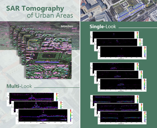
For the single-look case, it is expected the need of more tomograms to describe the complete structure of the edifice of the Bavarian state chancellery, thereby each contributing tomographic slice has significantly new meaningful information. Subsequently, we performed single-look TomoSAR for all polarizations (HH, HV and VV) on the three areas depicted by the green, red and blue lines crossing the ROI in Figure 5, but using the methodology suggested in Figure 1, i.e., DCRCB + WISE. For comparison purposes, we refer to the same TomoSAR focusing techniques as before, except for Capon, since it is no longer applicable.

This time we make use of three tomographic slices to describe the edifice of the Bavarian state chancellery. Figure 11, Figure 12 and Figure 13 show the single-look tomographic slices corresponding to the area depicted via the green line in Figure 5. Whereas Figure 14 presents the respective superimposed vertical profiles for each position within the displayed tomograms; the (pseudo) power is presented in a linear scale. Conversely, Figure 15, Figure 16 and Figure 17 depicts the single-look tomograms corresponding to the area depicted via the red line in Figure 5, crossing the ROI. As before, Figure 18 shows the respective superimposed vertical profiles for each position composing the displayed tomograms.

The results given by Figure 11, Figure 12 and Figure 13 depict the two wings composing the abovementioned edifice (enclosed by the blue rectangle in Figure 6), whereas the succeeding tomographic slices, given by Figure 15, Figure 16 and Figure 17, show part of the central building, as seen in Figure 6. As earlier, MSF presents worse resolution, higher ambiguity levels and numerous artifacts. On the other hand, the other treated more sophisticated approaches improve such aspects, being CS and WISE the techniques with best performance. Note that WISE remains as the method achieving finer resolution. This time, the solutions retrieved by DCRCB are the ones refined via statistical regularization, by means of the iterative process described in Algorithm 1. After convergence, enhanced reconstructions are attained.

Note that, for MSF and DCRCB, the set of tomograms depicting the wings of the selected edifice (Figure 11, Figure 12 and Figure 13) present high ambiguity levels among the PLOS height range from −35 m to 60 m and from −10 m to −20 m, with a pseudo-power up to −3 dB and −5 dB, respectively, in the VV polarization. CS and WISE perform reduction of the ambiguity levels; however, the presence of ambiguities is still significant in some positions, especially for VV, which may lead to false detections. The analysis of all polarizations and the succeeding tomograms helps discriminating these ambiguities. The latter makes more sense for the single-look case, since the spatial mixture of sources is avoided. Moreover, we can also compare the single-look response against the multilook response. By instance, the ambiguity levels for CS and WISE in Figure 11 (HH polarization), among the aforesaid PLOS height ranges, are weaker. Furthermore, these same ambiguities do not appear in the succeeding tomograms in Figure 15, Figure 16 and Figure 17. Without having a priori information on the ROI, we could infer that the sources within such ranges, for the VV polarization in Figure 13, are indeed ambiguities. Thus, the PLOS height range can be set accordingly, e.g., from −10 m to 30 m.

For completeness, Figure 19 shows the single-look tomographic slices corresponding to the area depicted via the blue line in Figure 5. These tomograms represent the dome encircled by the yellow dashed line in Figure 6. We refer only to the methodology suggested in Figure 1 (i.e., DCRCB + WISE) since its capabilities have been already verified. Consistently, Figure 20 presents the corresponding superimposed vertical profiles for each position composing the displayed tomograms; the (pseudo) power is presented in a linear scale.

An interesting aspect about the results given in Figure 19 and Figure 20 is the presence of a single dominant scatterer, which could be utilized to perform PSI. The study carried in [6] suggests combining single-look TomoSAR with a PSI approach toward the objective of improving deformation sampling in layover-affected urban areas. For such a purpose, the use of CS, as a super-resolution technique, is restricted to those pixels that contain closely spaced scatterers (classified a priori), due to the computational burden. The methodology introduced in this work is intended to replace CS; being much faster, it could be applied for the aims of [6] in a general basis, without the need of pre-classifying the pixels composing the illuminated scene.

Finally,

Table 2. Average Processing Time ¹.

TomoSAR Focusing Technique	Processing Time [s]
MSF	0.2290
Capon	0.2987
DCRCB	0.3663
CS	65.2083
Capon + WISE	4.5168
DCRCB + WISE	5.3092

¹ Performed in an Intel© Xeon© X7560 CPU at 2.27 GHz, using a single thread.

presents the average processing time to perform focusing of a single pixel, for all addressed TomoSAR focusing techniques. All methods are implemented in Python, using the CVXPY [26] and the CVXOPT [27] software libraries to solve the CS convex problem in (18). In order to take full advantage of the super-resolution capabilities of CS and WISE, we make use of $M=100$ samples to describe the estimated PSP $\widehat{b}$ (see Section 2). We consider the single-look case for all methods, excluding Capon.

5. Discussion

The goal of the introduced methodology is to achieve enhanced TomoSAR imaging of urban areas without the necessity of performing multilooking. In this scenario, multilooking is optionally used to deal with the random scattering responses, but not to guarantee well-conditioned (invertible) data covariance matrices.

One of the motivations of this work is to present an alternative to Capon beamforming, which results inapplicable when the data covariance matrices are rank deficient, and to CS, up to now one of the most used and reliable TomoSAR focusing techniques for urban scenarios, yet, computationally expensive.

Consequently, the introduced methodology suggests solving the nonlinear ill-conditioned TomoSAR inverse problem using statistical regularization approaches, in the context of the decision making theory. Particularly, the MARIA and WISE methods are considered; the first one inspired on ML and the second one based on the WCF criterion. These techniques offer several advantages, which include: (i) resolution enhancement; (ii) ambiguity levels reduction; (iii) suppression of artifacts; (iv) it is not necessary to know beforehand the number of sources sharing the same resolution cell.

The related ML and WCF optimization problems are solved analytically, leading to the possibility to adapt the respective solvers to specific circumstances. By instance, with the aim of preventing the spatial mixture of sources due to multilooking, this paper presents a variation of MARIA and WISE, which utilizes a robust version of Capon (i.e., DCRCB, NCCB and RCB) to provide them with its first input (zero-step iteration). In this way, we make use of the robust properties of DCRCB, NCCB and RCB, against the rank deficiencies of the involved data covariance matrices.

In order to demonstrate the capabilities of the given methodology, we refer to the worst case scenario: the single-look case. First, we refer to the area depicted via the red line in Figure 5. As a reference, we present the corresponding tomograms for the different addressed TomoSAR focusing techniques, after performing multilooking. Subsequently, we refer to the three areas depicted by the green, red and blue lines crossing the ROI in Figure 5. The corresponding tomographic slices for the single-look case are provided.

The first retrieved solutions, performing multilooking, already show the feature-enhancing properties of the selected (WISE) statistical regularization approach, in comparison to the other competing techniques: MSF, Capon, DCRCB and CS. We conclude that, when sufficient multilooking is provided, the use of Capon beamforming is recommended to provide WISE (or MARIA) with the first-input (zero-step iteration). Being the mathematical expression of Capon easier than its robust versions, it is easier to implement, having less computational burden.

On the other hand, when the data covariance matrices are not invertible, as for the single-look case, the use of a robust version of Capon is required to compute a first estimate of the PSP, which, later on, is to be refined using statistical regularization. For demonstration purposes, we make use of DCRCB as input to WISE. The respective tomograms show how WISE still performs feature-enhancement to a first PSP estimate, gotten using a different technique than Capon beamforming.

In general, the algorithm of WISE (and MARIA) allows using different techniques as an input, giving to the user the flexibility to adapt them for the different scenarios. It is recommended, however, the use of Capon beamforming and its robust versions, rather than any other methods, as explained in the following. MARIA and WISE retrieve approximate solutions to their respective minimization problems, being the “ideal” version of Capon the asymptotic. By ideal, we refer to Capon beamforming but using the true (modelled) data covariance matrix, instead of the sample covariance matrix. Therefore, for consistency reasons, it is advisable to use Capon as input, or in this case, one of its robust versions.

CS is a special case, which merits some discussion. The approach considered here is related to the covariance-matching minimization problem described in Equation (18), which is normally tackled using nonspecifically adapted convex optimization algorithms. By instance, for the presented work, the CVXPY [26] and CVXOPT [27] software libraries have been employed. Yet, not having an analytical solution causes some downsides, mentioned next: the tomograms retrieved via CS may present black fringes, since sometimes a solution to the TomoSAR problem cannot be found; the correct selection of ${\tau }_1$ and ${\tau }_2$ in Equation (18) produces a better response, however, the setting up of these parameters is not always straightforward.

Regularization parameter selection is customarily done using the L-curve method [28], the Morozov’s discrepancy principle [28] or the Stein’s unbiased risk estimate (SURE) [29]. These criteria are a posteriori, meaning that a comparison of different retrieved solutions with different regularization parameters is performed. The use of criteria like the aforementioned for tuning up the CS parameters results implausible. On one hand, CS incurs much more computation time in contrast to the other competing methods, due to the nonavailability of adapted efficient convex optimization algorithms and due to the iterative nature of such algorithms. On the other hand, modifying the different parameter selection tools to deal with the CS case, would involve having the analytical expression of the solver.

For these reasons, we consider CS impractical and we rather suggest using Capon beamforming or one of its robust versions (depending on the circumstances), along with MARIA or WISE to perform refinement of the previously retrieved solutions via statistical regularization.

Finally, future lines of research will focus on using better methods to perform multilooking rather than the standard Boxcar filtering. The use of nonlocal spatially adaptive filtering methods is a good option, which enhances the estimation of the covariance matrices, improving the scatterer separation in layover areas thanks to their smoothing and edge-preserving properties [30,31]. Another line of research is the use of ML to estimate the particular structures of the data covariance matrices, making them closer, in a statistical sense, to the true covariance matrices. Recall that most of the TomoSAR focusing algorithms are applied on an estimate of the actual data covariance matrices, obtained from a single independent realization.