Article

Comparison of CORINE Land Cover Data with National Statistics and the Possibility to Record This Data on a Local Scale—Case Studies from Slovakia

1
Department of Physical Geography and Geoecology, Faculty of Natural Sciences, Comenius University in Bratislava, Mlynská dolina, Ilkovičova 6, 842 15 Bratislava, Slovakia
2
Department of Ecology and Environmental Sciences, Faculty of Natural Sciences, Constantine the Philosopher University in Nitra, Tr. A. Hlinku 1, 949 01 Nitra, Slovakia
3
Department of Geography and Applied Geoinformatics, Faculty of Humanities and Natural Sciences, University of Prešov, 17. Novembra 1, 080 01 Prešov, Slovakia
4
Institute of Geography, Slovak Academy of Sciences, Štefánikova 49, 814 73 Bratislava, Slovakia
*
Author to whom correspondence should be addressed.
Remote Sens. 2020, 12(15), 2484; https://doi.org/10.3390/rs12152484
Submission received: 12 June 2020 / Revised: 27 July 2020 / Accepted: 29 July 2020 / Published: 3 August 2020

Abstract

:
Monitoring of land cover (LC) provides important information of actual land use (LU) and landscape dynamics. LC research results depend on the size of the area, purpose and applied methodology. CORINE Land Cover (CLC) data is one of the most important sources of LU data from a European perspective. Our research compares official CLC data (third hierarchical level of nomenclature at a scale of 1:100,000) and national statistics (NS) of LU in Slovakia between 2000 and 2018 at national, county, and local levels. The most significant differences occurred in arable land and permanent grassland, which is also related to the recording method and the development of agricultural land management. Due to the abandonment of agricultural areas, a real recorded increase in forest cover due to forest succession was not introduced in the official records of Land register. New modification of CLC methodology for identifying LC classes at a scale of 1:10,000 and fifth hierarchical level of CLC is firstly applied for local case studies representing lowland, basin, and mountain landscape. The size of the least identified and simultaneously recorded area was established at 0.1 ha the minimum width of a polygon was established at 10 m, the minimum recorded width of linear elements such as communications was established at 2 m. The use of the fifth CLC level in the case studies areas generated average boundary density 17.2 km/km2, comparing to the 2.6 km/km2 of the third level. Therefore, when measuring the density of spatial information by the polygon boundary lengths, the fifth level carries 6.6 times more information than the third level. Detailed investigation of LU affords better verification of national statistics data at a local level. This study also contributes to a more detailed recording of the current state of the Central European landscape and its changes.

Graphical Abstract

1. Introduction

Land use (LU) data and land cover (LC) monitoring are applicable at all government levels, from local government to European Union policy. Investigation of LU has many aspects, nowadays, the most important are LU planning aspects (classification of landscape in cadastral areas of rural municipalities and towns according to their use), the ownership record or Land Parcel Identification System (LPIS) for the purpose of controlling subsidies to farmers.
LU data registration has a historical development, which is in Central Europe connected with the introduction of the Theresian urbarium by Maria Theresa in 1767 and the creation of a land register in Slovakia. Since 1897, the Land register in Hungary has been recording parcels according to metric area and cadastral maps [1]. Actual Land Register data provided by Cadastral Portal of Geodesy, Cartography, and Cadastre Authority of the Slovak Republic records 10 types of parcels, data on ownership, area, use, conservation of nature, and cultural sites.
Land register focused on data on parcel types, which were mainly related to agricultural production (six types). The beginnings of LU research were also related to the inventorying of categories (parcel type), which were mainly related to ensuring food sovereignty [2]. This trend is confirmed by research on the Commission on Inventory of World Land Use, which began its activities at the 26th IGU Congress in Lisbon, or later LU research in Central and Eastern Europe, focusing specifically on agricultural LU [3].
Only remote sensing data have motivated research into other categories of land surface utilization with adequate classification systems [4,5]. The presented nomenclatures respected the functional and physiognomic features in the context of the tradition and conventions of geographic research by using aerial photographs and satellite images. In their identification and interpretation, the emphasis is usually placed on those features that characterize generally known objects of the Earth’s surface, most often refer to their physiognomic difference but also to their function and environmental (ecological) significance. Aerial photographs and satellite images, in particular with high parameters regarding spatial, spectral, and temporal resolution, contributed significantly to the land cover/land use (LC/LU) research. Remote sensing data makes it possible to identify LC/LU objects (both natural and human-generated) through physiognomic and morphological characteristics. They also indicate their third dimension [6]. These identified LC/LU objects provide information concerning the real physical state of the landscape. Current approaches to satellite images interpretation have been pointed out by Di Gregorio and Jansen [7], Comber et al. [8], and Feranec et al. [9].
The CORINE Land Cover (CLC) programme, which introduced a method of identifying land cover from satellite images with a resolution of 10–50 m, integrating aspects of LU [6,10,11,12]. Very high resolution (VHR) satellite images in the order of meters, such as IKONOS and QuickBird, are suitable for large scale research and land cover/use mapping. The basic disadvantage of satellite data processing is that it is necessary to pre-prepare data focused mainly on atmospheric correction, but also to eliminate the effects of cloud cover, which can significantly distort final outputs especially when applying semi-automated or automated procedures of LC segmentation. Aerial images can also be used in research with detailed legend and classification [13]. Data from CLC projects are the most important sources of LU data from a European perspective. The method for identifying and recording LC (so-called inventory) based on satellite images [10,12] was applied throughout CLC projects. Since 1990, the European Environment Agency (EEA) has coordinated its gradual application in most European countries. Currently, CLC data sets are part of The European Copernicus programme, previously known as Global Monitoring for Environment and Security (GMES) and EEA coordinate landscape monitoring services for the PAN-European region. Uniform legend and method of identification of 44 LC classes allow landscape changes research at a European level as well as within national regions [14]. The CLC product is a wall-to-wall LC map at a scale 1:100,000 for the entire territory of the European Union (EU) Member States and associate countries (currently 39 countries and approximately 5.8 million square kilometers). CLC is the most complete and consistent cartographic source of knowledge regarding changes that occurred in the European landscape during the reference period 1985–2012 [15], and a fifth version (CLC2018) is currently available and in its final validation stages [16,17].
The LC inventory was carried out by visual photo-interpretation, computer-assisted photo-interpretation and semi-automated satellite images methods [14]. The following satellites were used: Landsat TM and ETM, SPOT, IRS P6, RapidEye, Sentinel-2, and Landsat-8, and were accompanied by various auxiliary data, e.g., aerial photographs, thematic maps, etc. The advantages of CLC include a unified hierarchical legend allowing data comparability. The scale of the resulting maps on third hierarchical level of nomenclature CLC3 for years 1990, 2000, 2006, 2012, and 2018 is 1:100,000. The limiting factor for data usability on a local scale is the minimum size of the mapped area, which is 25 ha and the minimum width of line elements, which is 100 m. All CLC data layers are available on the EEA webpage: https://land.copernicus.eu/pan-european/corine-land-cover/view, or Spatial Data Registry (SDR): https://rpi.gov.sk/en. Their universal features and compatibility with other environmental data in European countries is evidenced by a number of works assessing landscape changes [18,19,20,21], development flows and landscape dynamics [15,22,23], fragmentation and its impact on the landscape [24,25,26], ecosystem services assessment [27,28]. Druga and Minár [29] used CLC data to interpret the exposure of landscape structure to human influence.
According to cadastral territories, LU records in Slovakia are carried out by the Geodesy, Cartography and Cadastre Authority of the Slovak Republic and published in Land Register. Land register update data for basic spatial units (parcels), especially in the context of legal documents concerning ownership, acreage, usage, and other related factors—for example protection of nature, landscape, and cultural monuments.
At the same time, the real estate cadastral cartographic documents in national statistics (NS) registers only 10 categories (parcel type) of LU without integrating information on environmental and spatial relationships—all important in the context of landscape planning and management. The need for a detailed landscape study on a local level, including its line elements and significant non-forest tree species, is also important from the perspective of its protection and the awareness of ecological services.
The dynamics of LC changes have also motivated research on a large scale with an effort to detail the CLC method and at the same time to approach the Land register data. In the Slovak conditions, it was several works that brought proposals for detailing the CLC method [30,31].
National statistics (NS) register provides data on changes in LU and land area in total values of land types every year. This data records the legal status of the parcels, which may not correspond to their real use. The family house on the building plot is only registered after the approval or abandoned agricultural pasture can by natural succession of woody vegetation to form forest land. Therefore, the legal status regarding the use of parcels does not correspond to their actual use recorded by aerial photographs and satellite images, e.g., also interpreted by the CLC method. The lack of CLC data was their regional scale (the minimum size of the mapped area—25 ha, and the minimum width of line elements—100 m), which is not comparable with NS data. This was also the motive and intention of the modification of the CLC method and its detailing to five hierarchical levels, to obtain current CLC5 data on the use of parcels. This accuracy of CLC data is their current advantage over NS data.
Several works from Slovakia compared CLC data at the third hierarchical level (on a regional scale) with data from Land register [32,33,34] or used data from both data sources to analyze agricultural transition [35] and suburbanization processes [36].
Increasing the accuracy and detail of CLC methodology will allow, on case studies on local scales, to identify LC/LU data that will be comparable to Land register data.
The aims of our paper are:
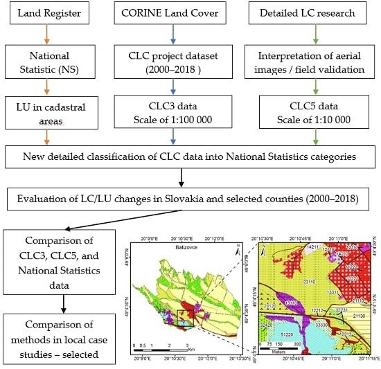
  • Comparing the development of LU changes on a base of relevant data sources in Slovakia and differences between CLC project outputs on a scale of 1:100,000 with three hierarchical levels of nomenclature (CLC3) and national statistics (NS) between 2000 and 2018, for the Slovak Republic, selected counties and municipalities.
  • Presenting the first application of the CLC methodology modification to identify and record LC classes on a scale of 1:10,000 with five hierarchical levels of nomenclature (CLC5) for local case studies representing lowland, basin, and mountain landscape.
  • Comparing the accuracy of LC research results (CLC5, CLC3) and NS in local case studies. Comparison is based on new detailed classification of LC classes into LU categories.

2. Materials and Methods

2.1. Data

2.1.1. Land Cover Data at a Scale 1:100,000 (CLC3)

Between 1990 and 2018, the following resources were used to identify LC units under the CLC projects (Table 1). We used CLC3 data at a scale of 1:100,000 for evaluation of LC development and LC/LU comparison at the level of the Slovak Republic (SR), chosen counties (Senec, Poprad, and Námestovo) and municipalities (Ivanka pri Dunaji, Batizovce, and Oravská Polhora).

2.1.2. Land Cover Data at a Scale of 1:10,000 (CLC5)

Digital orthophoto mosaic with the spatial resolution of 25 cm (https://www.geoportal.sk/en/zbgis/orthophotomosaic.html) was used for detailed mapping and analyses of land cover at the municipal level (CLC5). The aerial photographs of western part of Slovakia were taken in 2017 and of the central part in 2018.

2.1.3. National Statistics (NS)
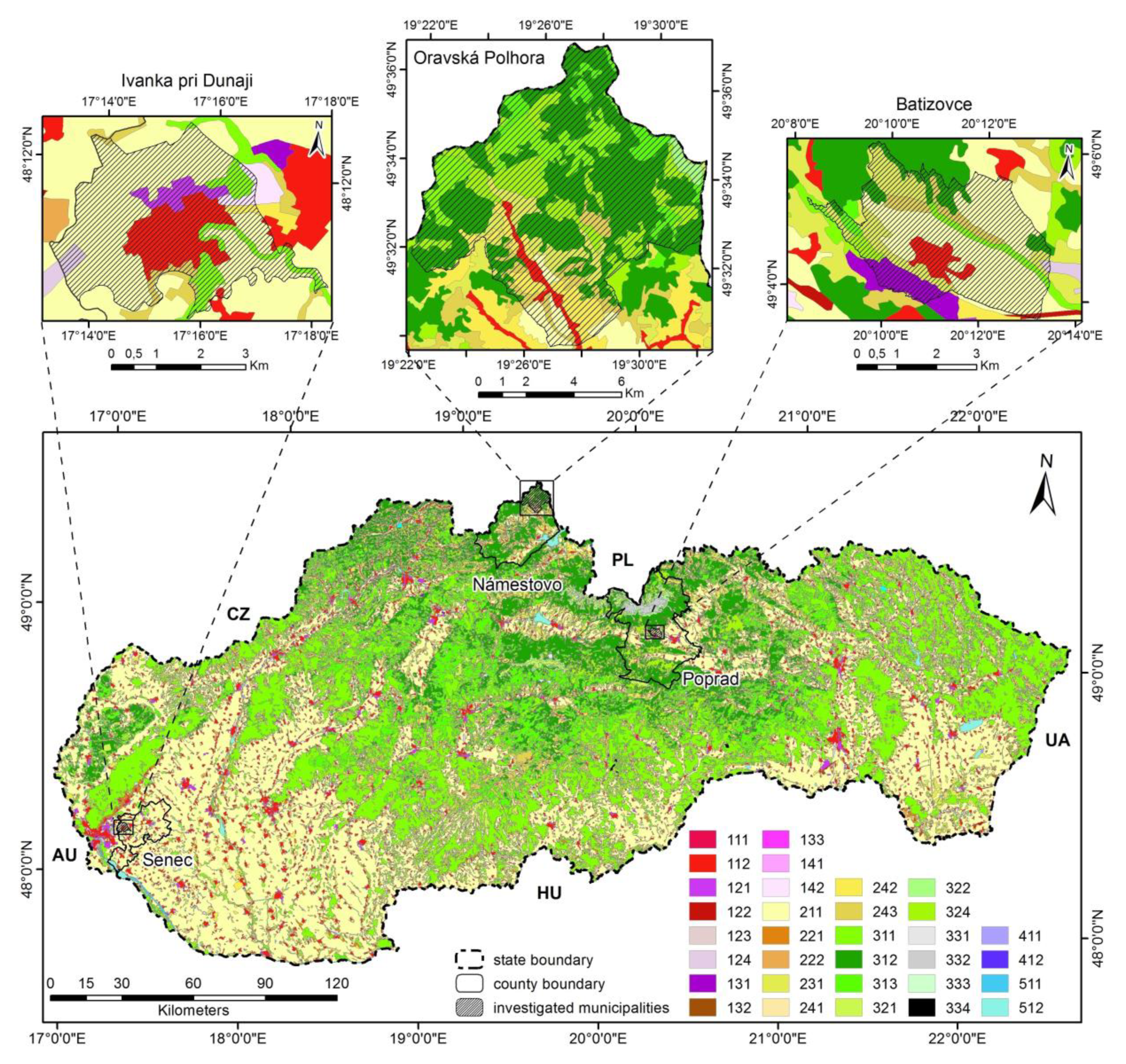
The observed LC data (CLC3 and CLC5) were compared with the area of individual categories of NS, which officially registers their current extent for cadastral areas. However, NS data is not spatially differentiated within the cadastral areas. The cadastral portal (http://www.katasterportal.sk/kapor/) lists the following LU categories in total values of land types: 1. Arable land, 2. Hop-fields, 3. Vineyards, 4. Gardens, 5. Orchards, 6. Permanent grassland, 7. Forest land, 8. Water areas, 9. Built-up areas and courtyards, and 10. Other areas. The data was obtained for the whole territory of the republic in the years 2000, 2006, 2012, and 2018 related to the CLC3 data layers. In particular, the accuracy of NS in 2018 for selected case studies was compared with CLC data and results of the detailed LC research.

2.2. Study Area

The Slovak Republic spans 49,035 km2 and has approximately 5.4 million residents [37]. It has been a member of the EU since 2004. Due to its location in Central Europe, the Carpathians and Pannonian Basin contribute to the division of its surface, which causes a variety of natural conditions. Case studies of detailed LC research (Figure 1) have been conducted to represent the basic types of lowland, basin, and mountain landscapes with residential, agricultural and forest LU.

2.2.1. Senec County—Municipality of Ivanka Pri Dunaji

Senec county with an area of 359.88 km2 and a population density of 245 inhabitants per square km is a part of the Bratislava self-governing region. The warm climatic region together with the predominant soil-forming substrate of fluvial sediments has meant there has been a significant potential for agricultural production and recreation in the vicinity of Sunny Lakes with an annual visitor rate of up to 1,000,000 tourists.
Ivanka pri Dunaji (Figure 1)—the proximity of Bratislava affected agricultural production (arable land, gardens, orchards, vineyards, and permanent grassland), localization of research institutes of Slovak Academy of Sciences and suburbanization. The municipality has an area of 14.26 km2 and is situated at an altitude of 128–133 m above sea level in the geomorphological unit of the Danube Plain, the Danube Lowland area.

2.2.2. Poprad County—Municipality of Batizovce

The Poprad district belongs to the Prešov self-governing region, has an area of 1105.38 km2 and an average population density of 95 per square km. Due to its biodiversity, there are 3 national parks (Tatra National Park, NP Low Tatras, and NP Slovak Paradise) with dominance of forest land.
Batizovce (Figure 1) is a municipality in the Podtatranská basin with an average height of 750 m above sea level and an area of 14.35 km2. Hilly relief on a paleogene base is predominant in this area. It was originally founded in the 13th Century as a village with forest management. Due to its basin position, agriculture predominated in the last century, especially the use of arable land and cattle grazing. The Batizovský brook flows from the Tatras through the municipality. Gravelly sand is mined on the fluvial sediments of floodplains.

2.2.3. Námestovo County—Municipality of Oravská Polhora

Námestovo county belongs to the Žilina self-governing region, has an area of 690.46 km2 with an average population density of 91 per square km. In the Orava region is dominated by mountainous relief, water bodies, electrotechnical industry, sub-mountain type of agricultural production, and forestry.
Oravská Polhora (Figure 1) is the northernmost municipality in the Slovak Republic, with the predominant montane and forest character in a cold climate area. It has an area of 84.47 km2 and is located in Oravské Beskydy. The highest point of Babia hora is 1725 m above sea level, the lowest point is the Polhoranka river floodplain which is 660 m above sea level. Oravská Polhora is one of the mountain settlements that were created due to Wallachian colonization waves.

2.3. Land Cover Interpretation at a Scale of 1:10,000

The universality of the CLC method and the applicability of data in different types of landscape research require specification of the nomenclature for the local scale. In this work we compare the areal accuracy of CLC3 with NS and carry out detailed LC research in three selected municipalities.
We used the method with theoretical background for identification and inventorying of land cover classes presented in Oťaheľ et al. [31], which represents modification of the CLC nomenclature on the 5th level for the detailed identification and tracking of LC at a scale of 1:10,000 (CLC5). Our method is based on the concepts and procedures applied to hierarchically higher classes [10,12,38]. Primarily, morpho-structural and physiognomic (appearance) attributes distinguishing individual landscape objects (areas) were respected. Along with their spatial relationships they make it possible to apply the association interpretation aspect and to differentiate objects (areas) by LU (function) attributes as well on a local level. The size of the least identified and simultaneously recorded area (Table 2) agrees with the study Druga et al. [30] who established it at 0.1 ha. It corresponds approximately to a square with a 31.5 m side, a circle with a 35.5 m diameter or a 20 × 50 m rectangle, as a compromise between the need for detail and the complexity of the drawing areas of LC in a GIS environment by using the computer-assisted photo-interpretation (CAPI) [14]. For practical reasons, the minimum width of a polygon has been derived from a scale of 10 m (1 mm in a map). The minimum change polygon was determined in an analogy to the generally applied CLC methodology of the third level as a fifth of the minimum identified area with the size of 0.02 ha [31]. The Atlas of Habitats of Slovakia (http://sbs.sav/atlas.html) was taken into account in the detailing of CLC3 classes of shrubs and/or herbaceous vegetation associations in order to create a nomenclature of CLC5. The nomenclature CLC5 respects the hierarchical levels of the CLC3 (10) and delimited LC units are marked with five-digit codes. In total, the CLC5 nomenclature contains 163 classes, of which 65 classes of Artificial surfaces, 34 Agricultural areas, 41 Forest land, 12 Wetland, and 11 Water bodies. In this work we identified 16 classes of artificial surfaces, 5 classes of agricultural land, 6 classes of forest land, and 5 classes of water bodies. Initial visual identification of land cover classes and delineation of their boundaries was realized using CAPI. As a basis for identification of the CLC5 at the municipality level a digital orthophoto mosaic of the Slovakia (https://www.geoportal.sk/en/zbgis/orthophotomosaic.html) was used. Individual aerial images taken in cloudless weather, representing the current state of the real spatial structure of the landscape, have already been rectified. The orthophoto mosaic was interpreted by the of CORINE Land Cover method modification and the nomenclature for identification and inventorying land cover classes at a scale of 1:10,000 [31]. The identified patterns of land cover were delimited in case studies using manual vectorization in ArcMap 10.7 (© ESRI) while respecting the minimum mapped area of 0.1 ha, minimum width of polygon 10 m and minimum recorded width of linear elements such a communications, accompanying vegetation and streams 2 m. The LC patterns show the spatial arrangement of objects on the Earth’s surface, while the textural characteristics serve to associate related identified areas into hierarchically arranged groups.
The quality of the LC interpretation was validated also during field survey. The LC classes were identified according to the characteristics of morpho-structural and physiognomic features, which distinguish the individual areas. These characteristics helped to differentiate the internal heterogeneity of CLC higher level classes. Several local characteristics cannot be obtained just by interpretation of aerial photographs (e.g., several functions of urbanized, agricultural, and semi-natural areas) and were complemented by detailed field research. The results of the field research, definitive delineation and identification of LC units served for final classification into a hierarchical structure within the CLC classes. The resulting CLC5 geodatabase was used to accurate data on LC and LU in local case studies.

2.4. Comparison of CLC Data and National Statistics

2.4.1. Classification of CLC Classes into National Statistics

The Table 3 shows the classification of individual CLC classes into the 3rd hierarchical level and the new proposal of the 5th CLC level [31] into the categories of national statistics. It was carried out by modifying and detailing the procedure according to Feranec [33].

2.4.2. Comparison of CLC3, CLC5, and National Statistics Data

A comparison of the current state and dynamics of LU in the Slovak Republic based on the interpretation of CLC3 data with registered land types according to NS of the Geodesy, Cartography and Cadastre Authority of Slovak Republic was carried out for the years 2000, 2006, 2012, and 2018. Similarly, CLC3 data for the years in question were compared at a county level for Senec, Poprad and Námestovo case studies. The CLC3 databases were downloaded from the Copernicus programme, specifically the CORINE Land Cover inventory. The layers were geoprocessed by clip tool to extract input features for Slovakia and selected counties for the above-mentioned years and for the municipality level only for the year 2018, respectively. As the clip features were used boundaries of territorial and administrative arrangement of the Slovak Republic in the basic level (© Geodetic and Cartographic Institute Bratislava).The total area of the individual land cover classes in the extracted CLC3 layers was calculated using the dissolve tool where the CLC codes in the attribute table were selected as the dissolve field and the area of these classes as the statistical field with the statistical sum operation. A detailed study of LC according to CLC5 [31] was carried out in case studies of these municipalities: Ivanka pri Dunaji, Batizovce, and Oravská Polhora. The results helped to refine LU data in 2018 and were compared with CLC3 and total values of land types from NS data.

2.4.3. Comparison of Spatial Accuracy of CLC3 and CLC5

To assess the increase of spatial detail of the detailed mapping, we compared the density of the boundaries of the classes mapped at 3rd and 5th CLC level (CLC3 and CLC5), as well as the density of the vertices of these boundaries. The lengths were calculated in ArcMap 10.6. using the Calculate Geometry tool and number of vertices by Feature Vertices To Points tool. Boundary lengths and number of vertices of all polygons in one layer were summated. We subtracted the length and number of vertices of the study area boundary, because it does not usually represent a LC boundary. We divided the resulting length and vertices number by two to ensure that each LC boundary is counted only once, despite the fact, that it has two geometrical representations in the GIS layer (by both adjacent polygons). Finally, we calculated several densities to assess different aspects of the spatial detail: boundary vertices per its length, boundary length per area, and total boundary vertices per area.

3. Results

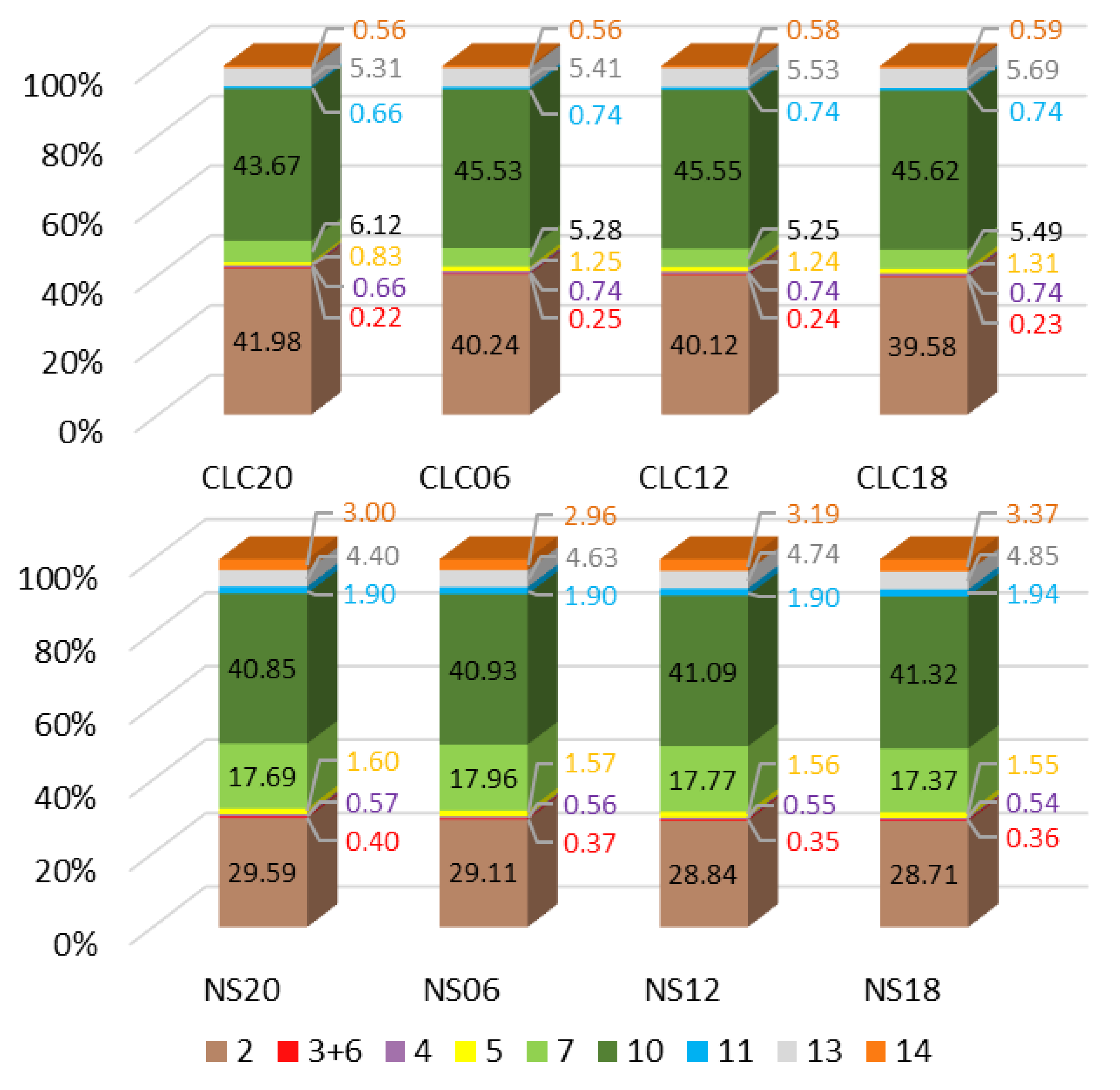
3.1. Development of LC Changes in Slovakia between 2000 and 2018

The most stable areas during 2000–2018, based on CLC3 data, include these types: water areas, vineyards, hop fields, and orchards. The built-up areas and courtyards slightly increased, mainly due to suburbanization trends during the transformation period. The forest land area has increased due to intensifying of agriculture and pasture overgrowth. The proportion of permanent grassland and arable land has simultaneously decreased slightly (Figure 2).
The largest deviations between CLC3 data and NS (Figure 2) are in the arable land category. CLC3 data also include, within this category, class 243 (Land principally occupied by agriculture, with significant areas of natural vegetation), which has a smaller arable land area. Relatively, the biggest differences are in the category of permanent grassland. NS data also register fodder (grassland) on arable land in this category; therefore, they have a larger area than CLC3. CLC3 data show the real state of agricultural land recorded by remote sensing, while the NS states the legal nature of the land [33]. Many grassland areas can be overgrown with woody vegetation after leaving farmland and changing to a transitional woodland/scrub class, i.e., forest land category. The CLC3 data show about 4% more forest land, considering the abandonment of agricultural land not yet officially registered. This trend in the abandonment of agricultural land is confirmed by several works [34,35,39]. The official Land register show more orchards and fewer vineyards, which corresponds to the differences in the evaluation of the real and officially led state. Several vineyards are already listed as building plots. These categories of LU showed a lack of CLC3 data (the smallest mapping unit 25 ha). Said shortcomings of CLC3 and NS data were the motive for detailing the CLC5 data.

3.2. Development of LC Changes between 2000 and 2018 in Chosen Counties

The Senec county (Figure 3) represents a suburban landscape near Bratislava, the capital city of Slovakia. The built-up area in the county has grown in the last 18 years thanks to development activities, while the share of arable land has decreased slightly. The area of orchards has grown, yet the share of vineyards and forests belonging to eco-stabilizing elements have reduced. The biggest differences were between the records of arable land. CLC3 data shows more arable land.
The Poprad county (Figure 4) is the most settled in the territory of the Podtatranská kotlina basin. The predominantly forested areas of the Tatras and the Low Tatras dominate. The most significant change was caused by wind calamity in 2004, which affected 126 km2 forest land but did not show up in NS because of invariably registered forest LU type. Arable land areas have a significantly higher representation in CLC3 than in the official records, where permanent grasslands prevail at their expense.
The Námestovo county (Figure 4) is one of the northernmost within the state and due to its climate, permanent crops are not grown. According to CLC3 data and NS forest land also covers the largest area, but CLC3 reports it at the expense of permanent grassland due to pasture overgrowth of up to 9% more than the NS records.

3.3. Cadastral Areas—Comparison of Methods

The municipality of Ivanka pri Dunaji retains the predominant character of suburban agricultural production with large-area fields and symptoms of suburbanization near the capital city of Bratislava. Using detailed land cover research (CLC5), the information on LU was specified, particularly in the municipality residential area, where areas of gardens next to single family houses were also recorded (Figure 5).
The municipality of Batizovce in a relatively small area represents various types of LU in its basin position. Detailed mapping shows areas of arable land, meadows, gravel pits, roads, and non-woody vegetation, which are in close proximity (Figure 5).
The territory of Oravská Polhora is very stable in terms of LU. Since 1949, three-quarters of the territory has remained the same. The most stable part is the northern half of the cadastral area, which is made up of forest. In this area there was only fragmentation of stands caused by forestry. Since this village is located in a marginal border position, it has not been intensively affected by urbanization. The municipality surroundings are a specific valuable archetype of the landscape, which is characterized by a symmetrical, fan-shaped arrangement of narrow-striped fields with a striped pattern in the direction of the slopes on both sides of the valley, in conditions of erosive relief of Podbeskydská brázda furrow (Figure 5).
Comparing the results of our own detailed mapping of the LC at a scale of 1:10,000 (CLC5) with the officially recorded values of NS and the official CLC3 data (Table 4 and Table 5), we can state that there is a generally higher concordance of NS in the built-up areas and gardens categories. The most significant differences occurred in arable land and permanent grassland, which is also related to the recording method and agricultural land management development. Due to the abandonment of agricultural areas, a real recorded increase of forest land due to woody vegetation succession was not introduced in the official records. Relatively, the Oravská Polhora records were the most accurate with only slight deviations between individual data. Due to the smaller spatial accuracy of the CLC database, smaller areas are not captured in it. This is particularly evident in water bodies, gardens, and the forest land.
Comparison of the spatial detail of the third and fifth CLC hierarchical levels used in the cadastral areas is stated in the Table 6. The use of the fifth CLC level in the case study areas generated average boundary density 17.2 km/km2, compared to the 2.6 km/km2 of the third level. Therefore, when measuring the density of spatial information by the polygon boundary lengths, the fifth level carries 6.6 times more information than the third level. Furthermore, there is not only more boundaries per area, but these boundaries are also drawn with higher point density—fifth CLC level uses more than three times more vertices per km of a boundary, than the third level. When put together as a density of the boundary vertices per area then the increase is more than twentyfold (45 vertices/km2 vs. 964 vertices/km2 in average). These densities have some differences among the study areas, which may be caused by different landscape, but also by the fact that the LC of each area was classified by a different person.

4. Discussion

The significance of CLC data from national to transnational level has been confirmed by numerous mentioned works [9,22,23,39]. Bielecka and Jenerowicz [40] manifest the intellectual and cognitive structure of CLC research applications on the example of analysis 873 documents from Web of Sciences during the period between 1985 and 2019. Authors concluded, that CLC data constitute a relatively young set of scientific data with a constant expansion and a strongly interdisciplinary structure. They point to the importance of research areas such as geography, remote sensing, ecology, forestry, agriculture, engineering, optics, and/or computer science, and they are convinced that this information could be very useful for CLC users, as it reflects a large-scale analysis of the CLC research lines and illuminates how research has changed over time in diverse areas of applications.
Moreover, in combination CLC data with data from NS were used in analyses of landscape changes [34,35]. Feranec [33] pointed out differences between CLC classes and NS types of LU. Nevertheless, at national level confirmed the proximity of CLC data sources for example, NS built up areas and courtyards with classes, CLC 11—urban fabric and CLC12—industrial, commercial, and transport units; or NS forest land with CLC 31—forests, 32—shrubs, and 324—transitional woodland/shrubs. For the forest land in NS, the legal status was decisive, unlike the real, physiognomic status they represent—transitional woodland/shrubs (324). There were big differences in the type of permanent grassland, which have a large variance in the CLC classes. In addition, under the NS, arable fodder crops are included in this type of land [33].
The accuracy of the recorded data on the types of land in NS is related to their legal status and not to their real mapped status in landscape. Such as e.g., no new suburbanization housing estates were registered in the development of the suburban landscape. This advantage of CLC data has been highlighted by Oťahel et al. [36]. Many buildings under construction, if not approved, are not recorded in the Land register.
The assessment of changes in LU development in historical contexts and the subsequent understanding of landscape management are based on LU/LC changes, and on CLC database [41]. Feng and Flewelling [42] point out that although LU/LC classes are commonly used in environmental modeling or landscape development, they might be taken as subjective information, and therefore their interpretation depends on the original purpose of the study and the quality of data sources.
LC data often serves as a basis for spatial decision-making [43]. They are currently being reflected in various regional and national evaluations. Their interpretations can be used to assess ecosystem services [43,44,45,46], biomass [47], the impact of EU subsidies [48], regional development [49,50,51,52,53,54,55,56], urbanization [57], the impact of climate change on the landscape [58], landscape protection [59,60,61,62,63,64], and many others. Our results are consistent with detailed mapping and comparisons in other European countries. Pflugmacher et al. [65] confirmed the differences between remote sensing data and real validated field data (LUCAS project) at the global European level. As in our country, the greatest differences are in the elements of deciduous forests, arable land, and permanent grassland. The need for data validation in landscape is also presented in other papers [66,67]. Data validation is also required in terms of identifying drivers of landscape change [68,69,70], landscape management [71], and hotspots of LU change [72].
The use of CLC5 methodology confirmed its applicability in terms of sufficient detailed mapping. It delimits LC classes reflecting detailed LU at local level and uses available aerial images in the visible spectrum. We can record individual adjacent, often contrasting classes of CLC not only in urbanized (e.g., discontinuous built-up areas and accompanying vegetation) but also in fragmented rural (detailed division of heterogeneous agricultural areas) and semi-natural landscape (transitional shrubs and young forests). Thus, it is possible to capture landscape variability without the need to use heterogeneous classes. This is important when comparing actual LU evidence between NS and CLC5.
Increase in the spatial resolution caused by the use of fifth CLC level instead of third level is significant (Table 6). The increase of detail of LC structure is documented by the 6.6 times increase of the boundary density, while the increase of detail of these boundaries is measured by 3.2 times increase of its vertex density. However, when employing a manual classification, the overall 20 times increase of the spatial information (vertex density-area) is proportional to the increase of a time needed to perform it. Therefore, this aspect should be considered and an acceptable ratio between the increase of spatial resolution and time demands should be set before each study using a detailed manual LC mapping. In the case of this study, the most important information derived from the mapping was the total area of each LC class and therefore the 6.6 times boundary density increase was essential. However, the cost of this increase was 20 times the increase in the amount of the vertices that had to be drawn.

5. Conclusions

CLC project is one of the most important sources of real LC/LU data. The advantages of CLC include its applicability to large territories and the comparability of the dynamics of landscape development of different types of landscapes. Scale of 1:100,000 and the size of minimum monitored area of 25 ha are suitable for national or regional studies. A comparison of the current state of land use in the Slovak Republic based on the interpretation of CLC data with registered land use according to the Geodesy, Cartography, and Cadastre Authority of Slovak Republic was carried out for 2000, 2006, 2012, and 2018. Similarly, CLC data for these years were compared at Slovakia as a whole and at county level for the Senec, Poprad, and Námestovo case studies. The most significant differences occurred in arable land and permanent grassland, which is also related to the recording method and agricultural land management development. The differences between the registrations of vineyards are related to the overgrowth of vineyards that do not correspond to the officially registered state.
Firstly, we used new modification of CLC methodology for identifying LC classes on a scale of 1:10,000 and the fifth hierarchical level of CLC nomenclature [31] for local case studies in this paper representing lowland (Ivanka pri Dunaji), basin (Batizovce), and mountain (Oravská Polhora) landscape. The size of the least identified and simultaneously recorded area was established at 0.1 ha. The minimum width of a polygon has been derived from a scale of 10 m (1 mm in a map). The minimum width of a line 2 m is based on the need to distinguish relevant barriers and corridors on a local scale. Roads, together with streams, channels, and riparian vegetation, represent areas with a surface mostly strongly contrasting with the surrounding landscape and have fundamentally different ecological properties.
We proposed new detailed classification of 163 LC types into LU categories usable for precise LC/LU comparisons. The use of the new modification on fifth CLC level in the case studies areas generated average boundary density 17.2 km/km2, compared to the 2.6 km/km2 on the third level (official CLC). When measuring the spatial detail more specifically as the density of the boundary vertices, then this increase is more than twentyfold. This not only means an increase of the boundary lines detail, but also with regard the time needed to perform the mapping and should therefore be considered before. Detailed investigation of LU affords better verification of NS data in a local level and helps to assess landscape spatial structures and ecological stability [73] on a large scale.
The use of the CLC5 methodology respects the characteristics of shrubs and herbaceous habitats [74] and can record agricultural land abandonment in large scale [75]. Our study also contributes to a more detailed recording of the current state of the Central European landscape, its changes and can be used for the prediction of its further development at the local level. While NS provide information on the legal state of parcels, LC data provide information on the real state of landscape. The increase in NS data inaccuracies occurs due to failure reports to the local administration, conditions for change of parcel type or the release of land due to an unknown owner. Detailed CLC5 data allows checking these spatial inaccuracies and reflects current landscape changes in local level.

Author Contributions

Conceptualization, V.F., F.P. and J.O.; methodology, V.F., J.O., J.F., J.N. and M.D.; data analyses and field investigation, F.P., M.H., V.S. and V.M.; visualization, M.H. and M.D.; data interpretation, V.F., J.O., F.P., J.F. and M.D.; writing—original draft, V.F., F.P., J.O., J.F., M.D. and J.N.; writing—review and editing, V.F., J.O., F.P., M.H. and M.D., supervision, V.F.; project administration, V.F. and F.P. All authors have read and agreed to the published version of the manuscript.

Funding

This publication was funded by Scientific Grant Agency of the Ministry of Education of the Slovak Republic and Slovak Academy of Sciences, the grant VEGA 1/0247/19 “Assessment of land-use dynamics and land cover changes”, and the grant VEGA 2/0023/19 “Land cover dynamics as an indicator of changes in the landscape”.

Conflicts of Interest

The authors declare no conflict of interest.

References

  1. Prikryl, Ľ.V. Vývoj Mapového Zobrazenia Slovenska; Veda: Bratislava, Slovakia, 1977. [Google Scholar]
  2. Stamp, D.L. The land utilization survey of Britain. Geogr. J. 1931, 78, 40–47. [Google Scholar] [CrossRef]
  3. Kostrowicki, J. Land use studies as a basis of agricultural typology of East-Central Europe. In Geographia Polonica 19. Essays on Agricultural Typology and Land Utilization; Kostrowicki, J., Tyszkiewicz, W., Eds.; Państwowe Wydawnictwo Naukowe: Warsaw, Poland, 1970; Volume 5. [Google Scholar]
  4. Anderson, J.R.; Hardy, E.E.; Roach, J.T.; Witmer, R.E. A Land Use and Land Cover Classification System for Use with Remote Sensor Data. US Geol. Surv. Prof. Pap. 1976, 964, 28. [Google Scholar]
  5. Baker, R.D.; De Steiger, J.F.; Grant, D.E.; Newton, M.J. Land use/land cover mapping from aerial photographs. Photogramm. Eng. Remote Sens. 1979, 45, 661–668. [Google Scholar]
  6. Feranec, J.; Ot’ahel’, J. Krajinná Pokrývka Slovenska (Land Cover of Slovakia); Veda: Bratislava, Slovakia, 2001. [Google Scholar]
  7. Di Gregorio, A.; Jansen, L.J.M. Land Cover Classification System: Classification Concepts and User Manual: LCCS. FAO Land and Water Development Division. 2000. Available online: http://www.fao.org/3/x0596e/x0596e01f.htm#p693%2059328 (accessed on 10 April 2020).
  8. Comber, A.; Fisher, P.; Waldsworth, R. What is land cover? Environ. Plann. B Plann. Des. 2005, 32, 199–209. [Google Scholar] [CrossRef] [Green Version]
  9. Feranec, J.; Hazeu, G.; Kosztra, B.; Arnold, S. CORINE land cover nomenclature. In European Landscape Dynamics: CORINE Land Cover Data; Feranec, J., Soukup, T., Hazeu, G., Jaffrain, G., Eds.; CRC Press: Boca Raton, FL, USA, 2016; pp. 17–25. [Google Scholar]
  10. Heymann, Y.; Steenmans, C.; Crossille, G.; Bossard, M. CORINE Land Cover: Technical Guide; Office for Official Publications of the European Communities: Luxembourg, 1994. [Google Scholar]
  11. Büttner, G.; Steenmans, C.; Bossard, M.; Feranec, J.; Kolář, J. The European CORINE land cover database. Int. Arch. Photogramm. Remote Sens. 1998, 32, 633–638. [Google Scholar]
  12. Bossard, M.; Feranec, J.; Ot’ahel’, J. CORINE Land Cover Technical Guide—Addendum 2000; EEA: Copenhagen, Denmark, 2000. [Google Scholar]
  13. Falťan, V.; Ot’ahel’, J.; Gábor, M.; Ružek, I. Metódy Výskumu Krajinnej Pokrývky (Methods of Land Cover Research); Comenius University: Bratislava, Slovakia, 2018. [Google Scholar]
  14. Feranec, J.; Feranec, J.; Soukup, T. Interpretation of satelite data. In European Landscape Dynamics: CORINE Land Cover Data; Feranec, J., Soukup, T., Hazeu, G., Jaffrain, G., Eds.; CRC Press: Boca Raton, FL, USA, 2016; pp. 33–40. [Google Scholar]
  15. Soukup, T.; Feranec, J.; Hazeu, G.; Jaffrain, G.; Jindrová, M.; Kopecký, M.; Orlitová, E.; Jupová, K. Trend of land cover changes in Europe in 1990–2012. In European Landscape Dynamics: CORINE Land Cover Data; Feranec, J., Soukup, T., Hazeu, G., Jaffrain, G., Eds.; CRC Press: Boca Raton, FL, USA, 2016; pp. 127–139. [Google Scholar]
  16. European Environmental Agency. Land Take during 2000–2018 and during the Corine Land Cover Observation Periods (2000–2006, 2006–2012, 2012–2018). Available online: https://www.eea.europa.eu/data-and-maps/explore-interactive-maps/land-take-2000-2018 (accessed on 19 April 2020).
  17. Martínez-Fernández, J.; Ruiz-Benito, P.; Bonet, A.; Gómez, C. Methodological variations in the production of CORINE land cover and consequences for long-term land cover change studies. The case of Spain. Int. J. Remote Sens. 2019, 40, 8914–8932. [Google Scholar] [CrossRef] [Green Version]
  18. Rogan, J.; Chen, D. Remote sensing technology for mapping and monitoring land-cover and land-use change. Prog. Plan. 2004, 61, 301–325. [Google Scholar] [CrossRef]
  19. Treitz, P.; Rogan, J. Remote sensing for mapping and monitoring land-cover and land-use change—An introduction. Prog. Plan. 2004, 61, 269–279. [Google Scholar] [CrossRef]
  20. Kuemmerle, T.; Radeloff, V.C.; Perzanowski, K.; Hostert, P. Cross-border comparison of land cover and landscape pattern in Eastern Europe using a hybrid classification technique. Remote. Sens. Environ. 2006, 103, 449–464. [Google Scholar] [CrossRef]
  21. Liga, J.; Petrovič, F.; Boltižiar, M. Land cover changes in Slovakia 1900–2006 related to the distance from industrial areas and economic development. Geograf. Čas. 2014, 66, 3–20. [Google Scholar]
  22. Feranec, J.; Hazeu, G.; Christensen, S.; Jaffrain, G. CORINE land cover change detection in Europe (case studies of the Netherlands and Slovakia). Land Use Policy 2007, 24, 234–247. [Google Scholar] [CrossRef]
  23. Feranec, J.; Jaffrain, G.; Soukup, T.; Hazeu, G. Determining changes and flows in European landscapes 1990–2000 using CORINE land cover data. Appl. Geogr. 2010, 30, 19–35. [Google Scholar] [CrossRef]
  24. Riitters, K.H.; Wickham, J.D.; O’Neill, R.V.; Jones, K.B.; Smith, E.R.; Coulston, J.W.; Wade, T.G.; Smith, J.H. Fragmentation of continental United States forests. Ecosystems 2002, 5, 0815–0822. [Google Scholar] [CrossRef]
  25. Vogt, P.; Riitters, K.H.; Estreguil, C.; Kozak, J.; Wade, T.G.; Wickham, J.D. Mapping spatial patterns with morphological image processing. Landsc. Ecol. 2007, 22, 171–177. [Google Scholar] [CrossRef]
  26. Jaeger, J.; Soukup, T.; Madrinan, L.; Schwick, C.H.; Kienast, F. Landscape Fragmentation in Europe; Joint EEA-FOEN report. EEA Report No 2/2011; European Environmental Agency: Copenhagen, Denmark, 2011. [Google Scholar]
  27. Kroll, F.; Müller, F.; Haase, D.; Fohrer, N. Rural–urban gradient analysis of ecosystem services supply and demand dynamics. Land Use Policy 2012, 29, 521–535. [Google Scholar] [CrossRef]
  28. Erhard, M.; Olah, B.; Banko, G.; Kleeschultek, S.; Abdul-Malak, D. Ecosystem mapping and assessment. In European Landscape Dynamics: CORINE Land Cover Data; Feranec, J., Soukup, T., Hazeu, G., Jaffrain, G., Eds.; CRC Press: Boca Raton, FL, USA, 2016; pp. 199–211. [Google Scholar]
  29. Druga, M.; Minár, J. Exposure to human influence—A geographical field approximating intensity of human influence on landscape structure. J. Maps 2018, 14, 486–493. [Google Scholar] [CrossRef] [Green Version]
  30. Druga, M.; Falťan, V.; Herichová, M. Návrh modifikácie metodiky CORINE Land Cover pre účely mapovania historických zmien krajinnej pokrývky na území Slovenska v mierke 1:10 000—Príkladová štúdia historického k.ú. Batizovce (The proposal of the modification of the CORINE Land Cover nomenclature for the purpose of historical land cover change mapping in the territory of Slovakia in the scale 1:10 000—Case study of historical cadastral area of Batizovce). Geogr. Cassoviensis 2015, 9, 7–34. [Google Scholar]
  31. Ot’ahel’, J.; Feranec, J.; Kopecká, M.; Falt’an, V. Modification of the CORINE Land Cover method and the nomenclature for identification and inventorying of land cover classes at a scale of 1:10 000 based on case studies conducted in the territory of Slovakia. Geograf. Čas. 2017, 69, 189–224. [Google Scholar]
  32. Feranec, J.; Šúri, M.; Ot’ahel’, J.; Cebecauer, T. Results of comparing the National Statistics of the Czech Republic, Hungary, Rumania and Slovakia with CORINE land cover data (in Slovak). Geod. Kartogr. Obzor 2001, 8–9, 209–213. [Google Scholar]
  33. Feranec, J. Land cover and land use of Slovakia in the context of national statistics and the CORINE land cover data. Acta Geogr. Univ. Comen. 2008, 50, 135–144. [Google Scholar]
  34. Oťaheľ, J.; Feranec, J.; Husár, K.; Kopecká, M. Landscape Changes in 1990–2006: Interpretation According to the CORINE Land Cover (CLC) Data and Selected Statistical Indicators (Bratislava Region). Geogr. Cassoviensis 2010, 4, 152–161. [Google Scholar]
  35. Spišiak, P.; Feranec, J.; Ot’ahel’, J.; Nováček, J. Transition in the agricultural and rural systems in Slovakia after 1989. In Contemporary Changes of Agriculture in East-Central Europe: Rural Studies 15; Banski, J., Bednarek, M., Eds.; Polish Geographical Society: Stanislav Leszczynski Institute of Geography and Spatial Organization PAS: Warsaw, Poland, 2008; pp. 121–146. [Google Scholar]
  36. Ot’ahel’, J.; Solár, V.; Matlovič, R.; Krokusová, J.; Pazúrová, Z.; Ivanová, M. Suburban landscape: Analyzes of manifestation of suburbanization in the hinterland of Prešov. Geograf. Čas. 2020, 72, 131–155. [Google Scholar]
  37. Government Office of the Slovak Republic. Available online: https://www.vlada.gov.sk/slovensko/ (accessed on 5 May 2020).
  38. Feranec, J.; Ot’ahel’, J. Mapping of land cover at scale 1:50 000: Draft of the nomenclature for the Phare countries. Geograf. Čas. 1999, 51, 19–44. [Google Scholar]
  39. Feranec, J.; Ot’ahel’, J.; Kopecká, M.; Nováček, J.; Pazúr, R. Krajinná Pokrývka Slovenska a Jej Zmeny v Období 1990–2012; Veda: Bratislava, Slovakia, 2018. [Google Scholar]
  40. Bielecka, E.; Jenerowicz, A. Intellectual Structure of CORINE Land Cover Research Applications in Web of Science: A Europe-Wide Review. Remote Sens. 2019, 11, 2017. [Google Scholar] [CrossRef] [Green Version]
  41. Kolejka, J.; Klimánek, M.; Fragner, B. Post-industrial landscape: The case of the Liberec region, Czech Republic. Morav. Geogr. Rep. 2011, 19, 3–17. [Google Scholar]
  42. Feng, C.; Flewelling, D.M. Assessment of semantic similarity between land use/land cover classification systems. Comput. Environ. Urban Syst. 2004, 28, 229–246. [Google Scholar] [CrossRef]
  43. Maes, J.; Egoh, B.; Willemen, L.; Liquete, C.; Vihervaara, P.; Schägner, J.P.; Grizzeti, B.; Drakou, E.G.; La Notte, A.; Zulian, G.; et al. Mapping ecosystem services for policy support and decision making in the European Union. Ecosyst. Serv. 2012, 1, 31–39. [Google Scholar] [CrossRef]
  44. Burkhard, B.; Kroll, F.; Müller, F.; Windhorst, W. Landscapes’ capacities to provide ecosystem services—A concept for land-cover based assessments. Landsc. Online 2009, 15, 1–22. [Google Scholar] [CrossRef]
  45. Burkhard, B.; Kandziora, M.; Hou, Y.; Müller, F. Ecosystem service potentials, flows and demands-concepts for spatial localisation, indication and quantification. Landsc. Online 2014, 34, 1–32. [Google Scholar] [CrossRef]
  46. Vrbičanová, G.; Kaisová, D.; Močko, M.; Petrovič, F.; Mederly, P. Mapping cultural ecosystem services enables better informed nature protection and landscape management. Sustainability 2020, 12, 2138. [Google Scholar] [CrossRef] [Green Version]
  47. Natarjan, K.; Latva-Käyrä, P.; Zyadin, A.; Pelkonen, P. New methodological approach for biomass resource assessment in India using GIS application and land use/land cover (LULC) maps. Renew. Sust. Energ. Rev. 2016, 63, 256–268. [Google Scholar] [CrossRef]
  48. Lesniewska-Napierala, K.; Nalej, M.; Napierala, T. The Impact of EU Grants Absorption on Land Cover Changes—The Case of Poland. Remote Sens. 2019, 11, 2359. [Google Scholar] [CrossRef] [Green Version]
  49. Belčáková, I. Strategic Environmental Assessment—An Instrument for Better Decision-Making towards Urban Sustainable Planning. Proc. Eng. 2016, 161, 2058–2061. [Google Scholar] [CrossRef] [Green Version]
  50. Boltižiar, M.; Olah, B.; Gallay, I.; Gallayová, Z. Transformation of the Slovak cultural landscape and its recent trends. In Landscape and Landscape Ecology; Proceedings of the 17th International Symposium on Landscape Ecology, Nitra, Slovakia, 27–29 May 2015; Halada, Ľ., Bača, A., Boltižiar, M., Eds.; Institute of Landscape Ecology, Slovak Academy of Sciences: Bratislava, Slovakia, 2016; pp. 57–67. [Google Scholar]
  51. Gerard, F.; Petit, S.; Smith, G.; Thomson, A.; Brown, N.; Manchester, S.; Wadsworth, R.; Bugar, G.; Halada, L.; Bezák, P.; et al. Land cover change in Europe between 1950 and 2000 determined employing aerial photography. Prog. Phys. Geogr. 2010, 34, 183–205. [Google Scholar] [CrossRef] [Green Version]
  52. Haladová, I.; Petrovič, F. Predicted development of the city of Nitra in Southwestern Slovakia based on land cover–Land use changes and socio-economic conditions. Appl. Ecol. Environ. Res. 2017, 15, 987–1008. [Google Scholar] [CrossRef]
  53. Schneider, J.; Ruda, A.; Venzlů, M. Development of the rural landscape: The Dačice region case study, Czechia. Geogr. Tech. 2019, 14, 84–96. [Google Scholar] [CrossRef] [Green Version]
  54. Skokanová, H.; Havlíček, M.; Klusáček, P.; Martinát, S. Five military training areas—Five different trajectories of land cover development? Case studies from the Czech Republic. Geogr. Cassoviensis 2017, 11, 201–213. [Google Scholar]
  55. Swiader, M.; Lin, D.; Szewrański, S.; Kazak, J.K.; Iha, K.; van Hoof, J.; Belčáková, I.; Altiok, S. The application of ecological footprint and biocapacity for environmental carrying capacity assessment: A new approach for European cities. Environ. Sci. Policy 2020, 105, 56–74. [Google Scholar] [CrossRef]
  56. Ustaoglu, E.; Aydinoglu, A.C. Regional Variations of Land-Use Development and Land-Use/Cover Change Dynamics: A Case Study of Turkey. Remote Sens. 2019, 11, 885. [Google Scholar] [CrossRef] [Green Version]
  57. Izakovičová, Z.; Petrovič, F.; Mederly, P. Long-term land use changes driven by urbanisation and their environmental effects (example of Trnava City, Slovakia). Sustainability 2017, 9, 1553. [Google Scholar] [CrossRef] [Green Version]
  58. Lekaj, E.; Teqja, Z.; Bani, A. The dynamics of land covers categories and the impact of climate change on ultramafic areas of Albania. Period. Mineral. 2019, 88, 223–234. [Google Scholar]
  59. Chrastina, P.; Trojan, J.; Župčan, L.; Tuska, T.; Hlásznik, P.P. Land use as a means of the landscape revitalisation: An example of the Slovak exploae of Tardoš (Hungary). Geogr. Cassoviensis 2019, 13, 121–140. [Google Scholar]
  60. Izakovičová, Z.; Miklós, L.; Miklósová, V. Integrative assessment of land use conflicts. Sustainability 2018, 10, 3270. [Google Scholar] [CrossRef] [Green Version]
  61. Muchová, Z.; Raškovič, V. Fragmentation of land ownership in Slovakia: Evolution, context, analysis and possible solutions. Land Use Policy 2020, 95, 104644. [Google Scholar] [CrossRef]
  62. Muchová, Z.; Tárníková, M. Land cover change and its influence on the assessment of the ecological stability. Appl. Ecol. Environ. Res. 2018, 16, 2169–2182. [Google Scholar] [CrossRef]
  63. Pechanec, V.; Brus, J.; Kilianová, H.; Machar, I. Decision support tool for the evaluation of landscapes. Ecol. Inform. 2015, 30, 305–308. [Google Scholar] [CrossRef]
  64. Petrovič, F.; Stránovský, P.; Muchová, Z.; Falťan, V.; Skokanová, H.; Havlíček, M.; Gábor, M.; Špulerová, J. Landscape-ecological optimization of hydric potential in foothills region with dispersed settlements. A case study of Nová Bošáca, Slovakia. Appl. Ecol. Environ. Res. 2017, 15, 379–400. [Google Scholar] [CrossRef]
  65. Pflugmacher, D.; Rabe, A.; Peters, M.; Hostert, P. Mapping pan-European land cover using Landsat spectral-temporal metrics and the European LUCAS survey. Remote Sens. Environ. 2019, 221, 583–595. [Google Scholar] [CrossRef]
  66. Fritz, S.; See, L.; Perger, C.; McCallum, I.; Schill, C.; Schepaschenko, D.; Duerauer, M.; Karner, M.; Dresel, C.; Laso-Bayas, J.-C.; et al. A global dataset of crowdsourced land cover and land use reference data. Sci. Data 2017, 4, 170075. [Google Scholar] [CrossRef] [Green Version]
  67. Olofsson, P.; Foody, G.M.; Stehman, S.V.; Woodcock, C.E. Making better use of accuracy data in land change studies: Estimating accuracy and area and quantifying uncertainty using stratified estimation. Remote Sens. Environ. 2013, 129, 122–131. [Google Scholar] [CrossRef]
  68. Kristensen, S.B.P.; Busck, A.G.; van der Sluis, T.; Gaube, V. Patterns and drivers of farm-level land use change in selected European rural landscapes. Land Use Policy 2016, 47, 786–799. [Google Scholar] [CrossRef]
  69. Levers, C.; Butsic, V.; Verburg, P.H.; Müller, D.; Kuemmerle, T. Drivers of changes in agricultural intensity in Europe. Land Use Policy 2016, 58, 380–393. [Google Scholar] [CrossRef] [Green Version]
  70. Pazúr, R.; Bolliger, J. Land changes in Slovakia: Past processes and future directions. Appl. Geogr. 2017, 85, 163–175. [Google Scholar] [CrossRef]
  71. Jepsen, M.R.; Kuemmerle, T.; Müller, D.; Erb, K.; Verburg, P.H.; Haberl, H.; Vesterager, J.P.; Andrič, M.; Antrop, M.; Austrheim, G.; et al. Transition in European land-management regimes between 1800 and 2010. Land Use Policy 2015, 49, 53–64. [Google Scholar] [CrossRef]
  72. Kuemmerle, T.; Levers, C.; Erb, K.; Estel, S.; Jepsen, M.R.; Müller, D.; Plutzar, C.; Stürck, J.; Verkerk, P.J.; Verburg, P.H.; et al. Hotspots of land use change in Europe. Environ. Res. Lett. 2016, 11, 064020. [Google Scholar] [CrossRef]
  73. Hruška, M.; Falt’an, V.; Ivanová, M. Implementation of alternative assessments of ecological stability of a landscape: A case study of the environmentally affected area of Rudňany. Geograf. Čas. 2019, 71, 141–159. [Google Scholar]
  74. Stanová, V.; Valachovič, M. Katalóg Biotopov Slovenska; Daphne, Inštitút Aplikovanej Ekológie: Bratislava, Slovakia, 2002. [Google Scholar]
  75. Pazúr, R.; Lieskovský, J.; Feranec, J.; Ot’ahel’, J. Spatial determinants of abandonment of large-scale arable lands and managed grasslands in Slovakia during the periods of post-socialist transition and European Union accession. Appl. Geogr. 2014, 54, 118–128. [Google Scholar] [CrossRef]
Figure 1. Localization of investigated counties and municipalities with the CORINE Land Cover (CLC3) inventory in the Slovak Republic in 2018. Legend of land cover classes is available at the following link: https://land.copernicus.eu/pan-european/corine-land-cover/clc2018.
Remotesensing 12 02484 g001
Figure 2. Development of relative land use (LU) values for the Slovak Republic according to recorded national statistics (NS) data and comparison with CLC3 data in 2000, 2006, 2012, and 2018. LU codes according to NS: 2 arable land, 3 hop fields, 4 vineyards, 5 gardens, 6 orchards, 7 permanent grassland, 10 forest land, 11 water areas, 13 built-up areas and courtyards, and 14 other areas.
Remotesensing 12 02484 g002
Figure 3. Development of relative LU values for the counties of Senec according to recorded national statistics (NS) and CLC3 data in 2000, 2006, 2012, and 2018. LU codes according to NS: 2 arable land, 3 hop fields, 4 vineyards, 5 gardens, 6 orchards, 7 permanent grassland, 10 forest land, 11 water bodies, 13 built-up areas and courtyards, and 14 other areas.
Remotesensing 12 02484 g003
Figure 4. Development of relative LU values for the counties of Poprad and Námestovo according to recorded NS and CLC3 data in 2000, 2006, 2012, and 2018, respectively. LU codes according to NS: 2 arable land, 5 gardens, 7 permanent grassland, 10 forest land, 11 water bodies, 13 built-up areas and courtyards, and 14 other areas.
Remotesensing 12 02484 g004
Figure 5. Case studies with the CLC5 maps in 2018 (left) and examples of the detail outputs of this mapping at a scale of 1:10,000 (right). The colours correspond to the legend in Figure 1 (see above).
Remotesensing 12 02484 g005
Table 1. Description of the source data for interpretation of land cover (CORINE Land Cover (CLC3)).
DatasetYear of AcquisitionSpatial ResolutionSourceFormat
CLC19901986–1998≤50 mLandsat-5 MSS/TMvector
CLC20002000 +/− 1 year≤25 mLandsat-7 ETMvector
CLC20062006 +/− 1 year≤25 mSPOT-4/5,
IRS P6 LISS III
vector
CLC20122012 +/− 1 year≤25 mIRS P6 LISS III, RapidEyevector
CLC20182018 +/− 1 year≤10 m
(Sentinel-2)
Sentinel-2,
Landsat-8
vector
Table 2. Comparison of the size of the minimum mapped CLC areas on the 3rd, 4th, and 5th hierarchical levels.
Map Scale1:100,0001:50,0001:10,000
Size of the least identified area (ha)2540.1
Minimum width of polygon (m)100502
Minimum change polygon (ha)510.02
Table 3. Classification of CLC classes into 10 categories of national statistics. Underlined codes of CLC3 classes are on the CLC5 level divided into 2 categories of national statistics.
National StatisticsCLC3CLC5
Arable land211, 24312122 (large industrial greenhouses), 21110, 21121, 21122, 21130, 21140,
Hop field22222231, 22232
Vineyard22122111, 22112, 22113, 22121, 22122, 22131, 22132, 22133, 22151, 22152
Garden24211222, 12,122 (small garden greenhouses), 24211, 24212, 24220
Fruit orchard22222211, 22212, 22221, 22222
Permanent grassland231, 321 (natural grass-herbaceous stands)23110, 23120, 32112, 32122
Forest land311, 312, 313, 321 (alpine meadows), 322 (heath stands and dwarf pine), 324, 33412213 (unpaved forest roads), 14221, 31110, 31120, 31130, 31140, 31210, 31220, 31230, 31240, 31310, 31320, 31330, 32111, 32121, 32211, 32212, 32251, 32252, 32410, 32420, 32430, 32441, 32442, 32443, 33410
Water body411 (marshes), 511, 51241111, 41112, 41113, 51110, 51120, 51210, 51220, 51230
Build-up area and courtyard111, 112, 121, 122, 123, 124, 13311111, 11112, 11211, 11212, 11213, 11221, 11240, 11250, 12111, 12112, 12113, 12114, 12115, 12116, 12121, 12131, 12140, 12211, 12212, 12214, 12215, 12221, 12222, 12223, 12311, 12312, 12331, 12332, 12411, 12421, 13311, 13312, 13313, 13314, 14222
Other area131, 132, 141, 142, 322 (shrubs), 331, 332, 333,
411 (wetlands), 412
11230, 12,115 (cemeteries without vegetation), 12117, 12123, 12132, 12,213 (unpaved roads outside the forest), 12231, 12232, 12233, 12412, 12422, 13110, 13120, 13211, 13212, 13220, 14111, 14112, 14120, 14130, 14211, 14212, 14213, 14214, 14223, 14224, 14225, 14230, 21151, 21152, 21153, 21154, 23131, 23132, 23133, 23134, 32220, 32231, 32232, 32233, 32240, 33110, 33120, 33130, 33211, 33212, 33310, 33320, 33330, 33340, 33350, 41120, 41130, 41140, 41211, 41212, 41213, 41221, 41222, 41230, 51131, 51132, 51133, 51241, 51242, 51243
Table 4. Comparison of NS, official CLC data (CLC3) and outputs of the newly proposed methodology for detailed mapping of LC (CLC5) for case studies of municipalities in 2018.
National StatisticsCodeIvanka pri DunajiBatizovceOravská Polhora
NSCLC5CLC3NSCLC5CLC3NSCLC5CLC3
Arable land253,4554,6753,5837,9647,5553,493,22,217,95
Hop field3000000000
Vineyard40,1100000000
Garden55,518,311,30,690,760,020,050,075,73
Fruit orchard60,770,30000000
Permanent grassland71,771,73023,3320,6516,4518,5118,375,68
Forest land109,1810,5218,8512,9717,6915,4574,0875,4278,29
Water body111,921,5501,351,6400,650,260
Build-up area and courtyard1318,0913,7624,436,095,316,811,82,162,35
Other area149,199,171,8317,616,397,781,71,50
Sum 100%100%100%100%100%100%100%100%100%
Table 5. Legend of Land Cover Codes in Figure 5 (right).
5th CLC LevelCode
1.1.2.2.1Discontinuous built-up area with single-family houses(11221)
1.1.2.2.2Gardens next to single-family houses(11222)
1.2.1.1.4Areas of schools and research centers(12114)
1.2.1.1.7Prevailingly cultivated greenery in areas of services(12117)
1.2.1.2.1Infrastructure of buildings and artificial surfaces(12121)
1.2.1.2.3Accompanying (grass and woody) vegetation in areas of production(12123)
1.2.2.1.2Roads with a paved surface(12212)
1.2.2.1.3Roads with an unpaved surface(12213)
1.2.2.2.1Railway tracks and railyards(12221)
1.2.2.3.2Accompanying prevailing shrub vegetation(12232)
1.2.2.3.3Accompanying prevailing tree vegetation(12233)
1.3.1.1Open extraction spaces(13110)
1.3.3.1.1Construction of residential areas(13311)
1.4.1.2Cemeteries in inner settlement territories(14120)
1.4.2.1.1Areas of sports with prevailing natural surfaces(14211)
1.4.2.1.2Buildings and areas of sports with artificial surfaces—e.g., halls and sport plots(14212)
2.1.1.1Small-block arable land prevailingly without dispersed woody vegetation(21110)
2.1.1.3Large-block arable land prevailingly without dispersed woody vegetation(31130)
2.2.2.1.1Cultivated (not overgrown) orchards(22211)
2.3.1.1Grass stands prevailingly without trees and shrubs(23110)
2.3.1.2Grass stands with dispersed trees and shrubs(23120)
3.1.2.1Coniferous forests with a continuous canopy(31210)
3.1.2.2Coniferous forests with a discontinuous canopy(31220)
3.2.2.3.1Prevailingly continuous blackthorn shrubs(32231)
3.2.2.5.1Prevailingly continuous dwarf pine stands(32251)
3.2.4.2Young forest(32420)
3.3.3.3Rare discontinuous grass-herbaceous vegetation on gravel(33330)
5.1.1.2Channels(51120)
5.1.1.3.3Bank tree vegetation of streams and channels(51133)
5.1.2.2Artificial water bodies(51220)
Table 6. The comparison of the spatial detail of the 3rd and 5th CLC level (CLC3 and CLC5) used in the cadastral areas.
Cadastral AreaVertex Density (line)Vertex Density Increase IndexBoundary DensityBoundary Density Increase IndexVertex Density (Area)Vertex Density Increase Index
[Vertices/km][km/km2][Vertices/km2]
CLC 3CLC 5CLC 3CLC 5CLC 3CLC 5
Ivanka pri Dunaji16.354.03.32.120.79.735111732.3
Batizovce18.348.52.73.019.16.55492717.2
Oravská Polhora17.558.13.32.616.36.34594520.8
All Areas17.556.13.22.617.26.64596421.3

