Linear and Non-Linear Models for Remotely-Sensed Hyperspectral Image Visualization


Abstract
:1. Introduction
2. Data and Methods
2.1. Hyperspectral Images
2.2. Linear Color Formation Model
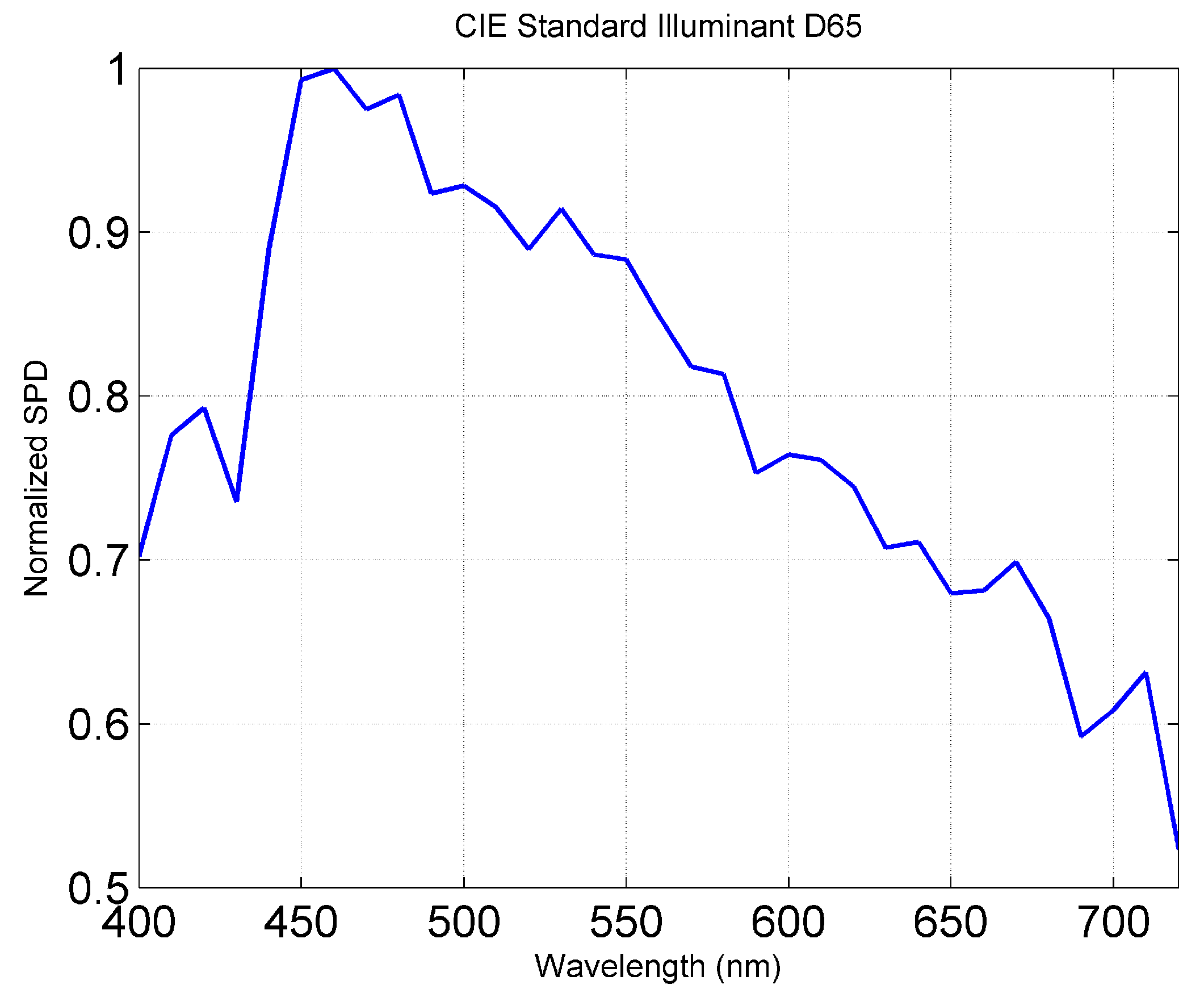
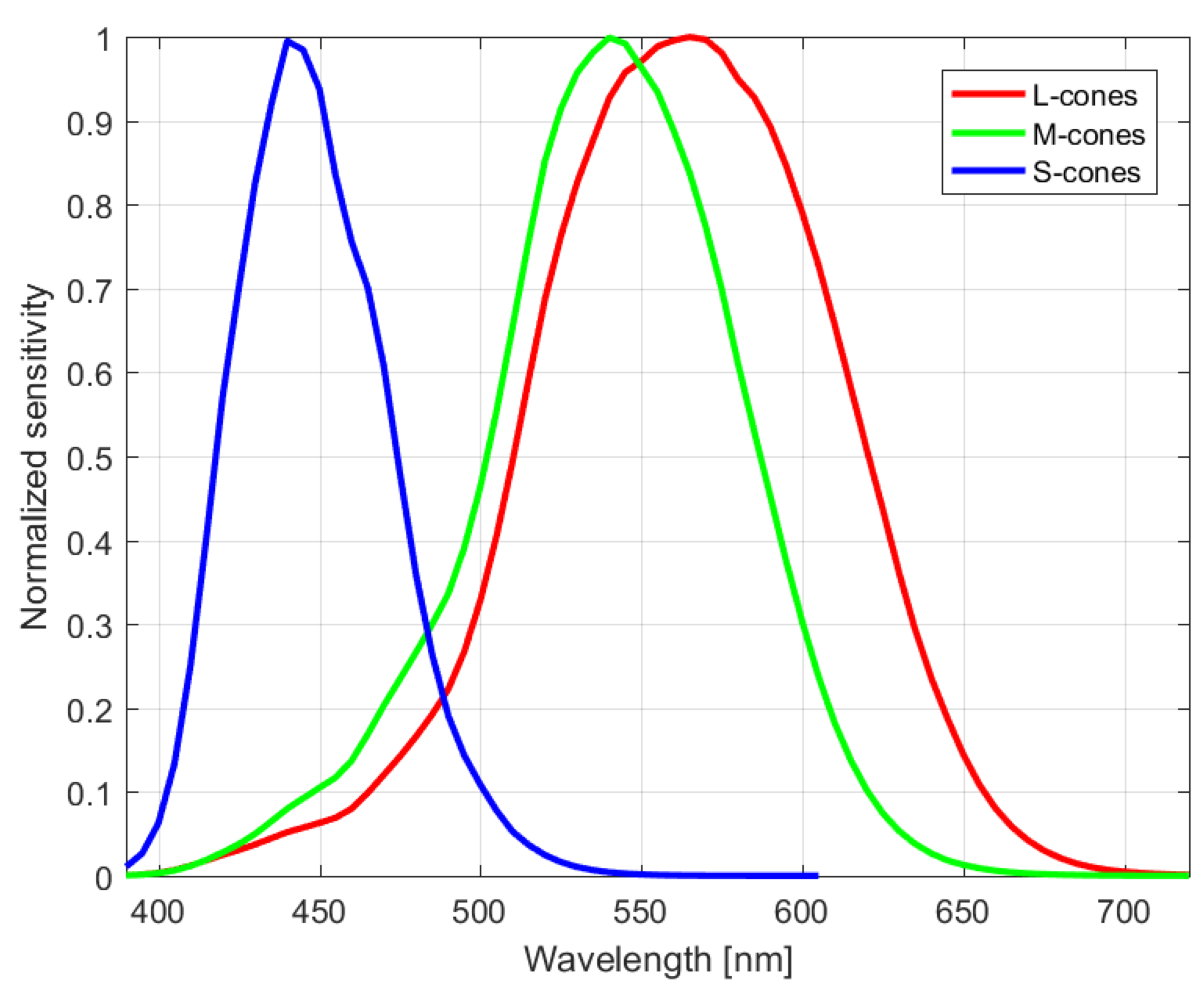
2.3. Spectral Sensitivity Functions
2.4. Non-Linear Color Formation Model
2.5. Quality Metrics
3. Experimental Results
4. Discussion
5. Conclusions
Author Contributions
Funding
Conflicts of Interest
References
- Kang, X.; Duan, P.; Li, S. Hyperspectral image visualization with edge-preserving filtering and principal component analysis. Inf. Fusion 2020, 57, 130–143. [Google Scholar] [CrossRef]
- Teke, M.; Deveci, H.S.; Haliloğlu, O.; Gürbüz, S.Z.; Sakarya, U. A short survey of hyperspectral remote sensing applications in agriculture. In Proceedings of the IEEE 2013 6th International Conference on Recent Advances in Space Technologies (RAST), Istanbul, Turkey, 12–14 June 2013; pp. 171–176. [Google Scholar]
- Reshma, S.; Veni, S. Comparative analysis of classification techniques for crop classification using airborne hyperspectral data. In Proceedings of the IEEE 2017 International Conference on Wireless Communications, Signal Processing and Networking (WiSPNET), Chennai, India, 22–24 March 2017; pp. 2272–2276. [Google Scholar]
- Piiroinen, R.; Heiskanen, J.; Maeda, E.; Viinikka, A.; Pellikka, P. Classification of tree species in a diverse African agroforestry landscape using imaging spectroscopy and laser scanning. Remote Sens. 2017, 9, 875. [Google Scholar] [CrossRef] [Green Version]
- Fricker, G.A.; Ventura, J.D.; Wolf, J.A.; North, M.P.; Davis, F.W.; Franklin, J. A convolutional neural network classifier identifies tree species in mixed-conifer forest from hyperspectral imagery. Remote Sens. 2019, 11, 2326. [Google Scholar] [CrossRef] [Green Version]
- Dumke, I.; Nornes, S.M.; Purser, A.; Marcon, Y.; Ludvigsen, M.; Ellefmo, S.L.; Johnsen, G.; Søreide, F. First hyperspectral imaging survey of the deep seafloor: High-resolution mapping of manganese nodules. Remote Sens. Environ. 2018, 209, 19–30. [Google Scholar] [CrossRef]
- Acosta, I.C.C.; Khodadadzadeh, M.; Tusa, L.; Ghamisi, P.; Gloaguen, R. A machine learning framework for drill-core mineral mapping using hyperspectral and high-resolution mineralogical data fusion. IEEE J. Sel. Top. Appl. Earth Obs. Remote Sens. 2019, 12, 4829–4842. [Google Scholar] [CrossRef]
- Shimoni, M.; Haelterman, R.; Perneel, C. Hypersectral Imaging for Military and Security Applications: Combining Myriad Processing and Sensing Techniques. IEEE Geosci. Remote Sens. Mag. 2019, 7, 101–117. [Google Scholar] [CrossRef]
- El-Sharkawy, Y.H.; Elbasuney, S. Hyperspectral imaging: A new prospective for remote recognition of explosive materials. Remote Sens. Appl. Soc. Environ. 2019, 13, 31–38. [Google Scholar] [CrossRef]
- Liao, D.; Chen, S.; Qian, Y. Visualization of Hyperspectral Images Using Moving Least Squares. In Proceedings of the IEEE 2018 24th International Conference on Pattern Recognition (ICPR), Beijing, China, 20–24 August 2018; pp. 2851–2856. [Google Scholar]
- Available online: https://www.harrisgeospatial.com/Software-Technology/ENVI/ (accessed on 23 July 2020).
- Demir, B.; Celebi, A.; Erturk, S. A low-complexity approach for the color display of hyperspectral remote-sensing images using one-bit-transform-based band selection. IEEE Trans. Geosci. Remote Sens. 2008, 47, 97–105. [Google Scholar] [CrossRef]
- Le Moan, S.; Mansouri, A.; Voisin, Y.; Hardeberg, J.Y. A constrained band selection method based on information measures for spectral image color visualization. IEEE Trans. Geosci. Remote Sens. 2011, 49, 5104–5115. [Google Scholar] [CrossRef] [Green Version]
- Su, H.; Du, Q.; Du, P. Hyperspectral imagery visualization using band selection. In Proceedings of the IEEE 2012 4th Workshop on Hyperspectral Image and Signal Processing: Evolution in Remote Sensing (WHISPERS), Shanghai, China, 4–7 June 2012; pp. 1–4. [Google Scholar]
- Tyo, J.S.; Konsolakis, A.; Diersen, D.I.; Olsen, R.C. Principal-components-based display strategy for spectral imagery. IEEE Trans. Geosci. Remote Sens. 2003, 41, 708–718. [Google Scholar] [CrossRef] [Green Version]
- Cui, M.; Razdan, A.; Hu, J.; Wonka, P. Interactive hyperspectral image visualization using convex optimization. IEEE Trans. Geosci. Remote Sens. 2009, 47, 1673–1684. [Google Scholar]
- Khan, H.A.; Khan, M.M.; Khurshid, K.; Chanussot, J. Saliency based visualization of hyper-spectral images. In Proceedings of the 2015 IEEE International Geoscience and Remote Sensing Symposium (IGARSS), Milan, Italy, 26–31 July 2015; pp. 1096–1099. [Google Scholar]
- Jacobson, N.P.; Gupta, M.R. Design goals and solutions for display of hyperspectral images. IEEE Trans. Geosci. Remote Sens. 2005, 43, 2684–2692. [Google Scholar] [CrossRef]
- Jacobson, N.P.; Gupta, M.R.; Cole, J.B. Linear fusion of image sets for display. IEEE Trans. Geosci. Remote Sens. 2007, 45, 3277–3288. [Google Scholar] [CrossRef]
- Fang, J.; Qian, Y. Local detail enhanced hyperspectral image visualization. In Proceedings of the 2015 IEEE International Geoscience and Remote Sensing Symposium (IGARSS), Milan, Italy, 26–31 July 2015; pp. 1092–1095. [Google Scholar]
- Kang, X.; Duan, P.; Li, S.; Benediktsson, J.A. Decolorization-based hyperspectral image visualization. IEEE Trans. Geosci. Remote Sens. 2018, 56, 4346–4360. [Google Scholar] [CrossRef]
- Zhang, B.; Yu, X. Hyperspectral image visualization using t-distributed stochastic neighbor embedding. In MIPPR 2015: Remote Sensing Image Processing, Geographic Information Systems, and Other Applications; Liu, J., Sun, H., Eds.; International Society for Optics and Photonics, SPIE: Bellingham, WA, USA, 2015; Volume 9815, pp. 14–21. [Google Scholar]
- Ertürk, S.; Süer, S.; Koç, H. A high-dynamic-range-based approach for the display of hyperspectral images. IEEE Geosci. Remote Sens. Lett. 2014, 11, 2001–2004. [Google Scholar] [CrossRef]
- Long, Y.; Li, H.C.; Celik, T.; Longbotham, N.; Emery, W.J. Pairwise-Distance-Analysis-Driven Dimensionality Reduction Model with Double Mappings for Hyperspectral Image Visualization. Remote Sens. 2015, 7, 7785–7808. [Google Scholar] [CrossRef] [Green Version]
- Liao, D.; Qian, Y.; Tang, Y.Y. Constrained manifold learning for hyperspectral imagery visualization. IEEE J. Sel. Top. Appl. Earth Obs. Remote Sens. 2018, 11, 1213–1226. [Google Scholar] [CrossRef] [Green Version]
- Jordan, J.; Angelopoulou, E. Hyperspectral image visualization with a 3-D self-organizing map. In Proceedings of the 2013 5th Workshop on Hyperspectral Image and Signal Processing: Evolution in Remote Sensing (WHISPERS), Gainesville, FL, USA, 26–28 June 2013; pp. 1–4. [Google Scholar]
- Duan, P.; Kang, X.; Li, S.; Ghamisi, P. Multichannel pulse-coupled neural network-based hyperspectral image visualization. IEEE Trans. Geosci. Remote Sens. 2019, 58, 2444–2456. [Google Scholar] [CrossRef]
- Duan, P.; Kang, X.; Li, S. Convolutional Neural Network for Natural Color Visualization of Hyperspectral Images. In Proceedings of the IGARSS 2019–2019 IEEE International Geoscience and Remote Sensing Symposium, Yokohama, Japan, 28 July–2 August 2019; pp. 3372–3375. [Google Scholar]
- Tang, R.; Liu, H.; Wei, J.; Tang, W. Supervised learning with convolutional neural networks for hyperspectral visualization. Remote Sens. Lett. 2020, 11, 363–372. [Google Scholar] [CrossRef]
- Shannon, C. A mathematical theory of communication. Bell Syst. Tech. J. 1948, 27, 379–623. [Google Scholar] [CrossRef] [Green Version]
- Amankwah, A. A Multivariate Gradient and Mutual Information Measure Method for Hyperspectral Image Visualization. In Proceedings of the IGARSS 2018–2018 IEEE International Geoscience and Remote Sensing Symposium, Valencia, Spain, 22–27 July 2018; pp. 5001–5004. [Google Scholar]
- Computational Intelligence Group of the University of the Basque Country (UPV/EHU). Hyperspectral Remote Sensing Scenes. 2014. Available online: http://www.ehu.eus/ccwintco/index.php/Hyperspectral_Remote_Sensing_Scenes (accessed on 23 July 2020).
- Buschner, R.; Doerffer, R.; van der Piepen, H. Imaging Spectrometer ROSIS. In Laser/Optoelektronik in der Technik / Laser/Optoelectronics in Engineering; Waidelich, W., Ed.; Springer: Berlin/Heidelberg, Germany, 1990; pp. 368–373. [Google Scholar]
- Vane, G.; Green, R.O.; Chrien, T.G.; Enmark, H.T.; Hansen, E.G.; Porter, W.M. The airborne visible/infrared imaging spectrometer (AVIRIS). Remote Sens. Environ. 1993, 44, 127–143. [Google Scholar] [CrossRef]
- Gu, J.; Jiang, J.; Susstrunk, S.; Liu, D. What is the Space of Spectral Sensitivity Functions for Digital Color Cameras? In WACV ’13, Proceedings of the 2013 IEEE Workshop on Applications of Computer Vision (WACV), Clearwater Beach, FL, USA, 15–17 January 2013; IEEE Computer Society: Washington, DC, USA, 2013; pp. 168–179. [Google Scholar]
- CIE Standard Colorimetric System. In Colorimetry; John Wiley & Sons, Ltd.: Hoboken, NJ, USA, 2006; Chapter 3; pp. 63–114.
- Kishino, K.; Sakakibara, N.; Narita, K.; Oto, T. Two-dimensional multicolor (RGBY) integrated nanocolumn micro-LEDs as a fundamental technology of micro-LED display. Appl. Phys. Express 2019, 13, 014003. [Google Scholar] [CrossRef]
- Stockman, A.; Sharpe, L.T. The spectral sensitivities of the middle-and long-wavelength-sensitive cones derived from measurements in observers of known genotype. Vis. Res. 2000, 40, 1711–1737. [Google Scholar] [CrossRef] [Green Version]
- Haykin, S.S. Neural Networks and Learning Machines, 3rd ed.; Pearson Education: Upper Saddle River, NJ, USA, 2009. [Google Scholar]
- Clevert, D.; Unterthiner, T.; Hochreiter, S. Fast and Accurate Deep Network Learning by Exponential Linear Units (ELUs). In Proceedings of the 4th International Conference on Learning Representations, ICLR, San Juan, Puerto Rico, 2–4 May 2016. [Google Scholar]
- Trottier, L.; Gigu, P.; Chaib-draa, B. Parametric exponential linear unit for deep convolutional neural networks. In Proceedings of the 2017 16th IEEE International Conference on Machine Learning and Applications (ICMLA), Cancun, Mexico, 18–21 December 2017; pp. 207–214. [Google Scholar]
- Paszke, A.; Gross, S.; Massa, F.; Lerer, A.; Bradbury, J.; Chanan, G.; Killeen, T.; Lin, Z.; Gimelshein, N.; Antiga, L.; et al. Pytorch: An imperative style, high-performance deep learning library. In Advances in Neural Information Processing Systems; NIPS: San Diego, CA, USA, 2019; pp. 8026–8037. [Google Scholar]
- McCamy, C.S.; Marcus, H.; Davidson, J.G. A Color-Rendition Chart. J. Appl. Photogr. Eng. 1976, 2, 95–99. [Google Scholar]
- Pascale, D. RGB Coordinates of the Macbeth ColorChecker; The BabelColor Company: Montreal, QC, Canada, 2006. [Google Scholar]
- Baldridge, A.; Hook, S.; Grove, C.; Rivera, G. The ASTER spectral library version 2.0. Remote Sens. Environ. 2009, 113, 711–715. [Google Scholar] [CrossRef]
- Pham, T.D. The Kolmogorov-Sinai Entropy in the Setting of Fuzzy Sets for Image Texture Analysis and Classification. Pattern Recognit. 2016, 53, 229–237. [Google Scholar] [CrossRef]
- Haralick, R.M.; Shanmugam, K.; Dinstein, I. Textural Features for Image Classification. IEEE Trans. Syst. Man Cybern. 1973, SMC-3, 610–621. [Google Scholar] [CrossRef] [Green Version]
- Ivanovici, M.; Richard, N. Entropy versus fractal complexity for computer-generated color fractal images. In Proceedings of the 4th CIE Expert Symposium on Colour and Visual Appearance, Prague, Czech Republic, 6–7 September 2016. [Google Scholar]
- Mandelbrot, B. The Fractal Geometry of Nature; W.H. Freeman and Co.: New York, NY, USA, 1982. [Google Scholar]
- Peitgen, H.; Saupe, D. The Sciences of Fractal Images; Springer: Berlin, Germany, 1988. [Google Scholar]
- Chen, W.; Yuan, S.; Hsiao, H.; Hsieh, C. Algorithms to estimating fractal dimension of textured images. IEEE Int. Conf. Acoust. Speech Signal Process. ICASSP 2001, 3, 1541–1544. [Google Scholar]
- Forsythe, A.; Nadal, M.; Sheehy, N.; Cela-Conde, C.; Sawey, M. Predicting beauty: Fractal dimension and visual complexity in art. Br. J. Psychol. 2011, 102, 49–70. [Google Scholar] [CrossRef] [Green Version]
- Falconer, K. Fractal Geometry, Mathematical Foundations and Applications; John Wiley and Sons: Hoboken, NJ, USA, 1990. [Google Scholar]
- Voss, R. Random Fractals: Characterization and measurement. Scaling Phenom. Disord. Syst. 1986, 10, 51–61. [Google Scholar] [CrossRef]
- Keller, J.; Chen, S. Texture Description and segmentation through Fractal Geometry. Comput. Vis. Graph. Image Process. 1989, 45, 150–166. [Google Scholar] [CrossRef]
- Maragos, P.; Sun, F. Measuring the fractal dimension of signals: Morphological covers and iterative optimization. IEEE Trans. Signal Process. 1993, 41, 108–121. [Google Scholar] [CrossRef]
- Allain, C.; Cloitre, M. Characterizing the lacunarity of random and deterministic fractal sets. Phys. Rev. A 1991, 44, 3552–3558. [Google Scholar] [CrossRef] [PubMed]
- Manousaki, A.; Manios, A.; Tsompanaki, E.; Tosca, A. Use of color texture in determining the nature of melanocytic skin lesions—A qualitative and quantitative approach. Comput. Biol. Med. 2006, 36, 416–427. [Google Scholar] [CrossRef]
- Ivanovici, M.; Richard, N. Fractal Dimension of Colour Fractal Images. IEEE Trans. Image Process. 2011, 20, 227–235. [Google Scholar] [CrossRef]
- Zhao, X.; Wang, X. Fractal Dimension Estimation of RGB Color Images Using Maximum Color Distance. Fractals 2016, 24, 1650040. [Google Scholar] [CrossRef]
- Nayak, S.R.; Mishra, J.; Khandual, A.; Palai, G. Fractal dimension of RGB color images. Optik 2018, 162, 196–205. [Google Scholar] [CrossRef]
- Li, J.; Du, Q.; Sun, C. An improved box-counting method for image fractal dimension estimation. Pattern Recognit. 2009, 42, 2460–2469. [Google Scholar] [CrossRef]
- Ivanovici, M. Fractal Dimension of Color Fractal Images with Correlated Color Components. IEEE Trans. Image Process. 2020. [Google Scholar] [CrossRef]
- Ivanovici, M. Color Fractal Images with Independent RGB Color Components. 2019. Available online: https://ieee-dataport.org/open-access/color-fractal-images-independent-rgb-color-components (accessed on 30 July 2020).
- Ivanovici, M.; Richard, N. A Naive Complexity Measure for color texture images. In Proceedings of the 2017 International Symposium on Signals, Circuits and Systems (ISSCS), lasi, Romania, 13–14 July 2017; pp. 1–4. [Google Scholar]
- Wang, Z.; Bovik, A.C.; Sheikh, H.R.; Simoncelli, E.P. Image quality assessment: From error visibility to structural similarity. IEEE Trans. Image Process. 2004, 13, 600–612. [Google Scholar] [CrossRef] [Green Version]
- Srivastava, N.; Hinton, G.; Krizhevsky, A.; Sutskever, I.; Salakhutdinov, R. Dropout: A simple way to prevent neural networks from overfitting. J. Mach. Learn. Res. 2014, 15, 1929–1958. [Google Scholar]


| Pavia University | Pavia Centre | ||||
|---|---|---|---|---|---|
| Method | |||||
| Linear Gaussian (proposed) | BS | 13.22 | 2.41 | 13.48 | 2.44 |
| NOL | 12.81 | 2.39 | 13.08 | 2.39 | |
| SOL | 12.68 | 2.38 | 12.96 | 2.38 | |
| MOL | 12.45 | 2.37 | 12.70 | 2.37 | |
| HOL | 10.79 | 2.35 | 10.82 | 2.36 | |
| Linear Camera (proposed) | Canon 5D | 12.03 | 2.37 | 12.10 | 2.36 |
| Canon 1D | 12.23 | 2.37 | 12.31 | 2.37 | |
| Hasselblad H2 | 12.25 | 2.38 | 12.25 | 2.37 | |
| Nikon D3X | 12.30 | 2.38 | 12.34 | 2.37 | |
| Nikon D50 | 12.45 | 2.38 | 12.49 | 2.38 | |
| ANN (proposed) | 15.38 | 3.02 | 15.28 | 2.87 | |
| PCA [15] | 15.20 | 2.84 | 14.58 | 2.75 | |
| CMF [18] | 14.98 | 2.51 | 15.11 | 2.63 | |
| CML [25] | 12.79 | 2.80 | 12.94 | 2.63 | |
| DHV [21] | 15.31 | 2.84 | 15.21 | 2.77 | |
| Indian Pines | Salinas A | Cuprite | |||||
|---|---|---|---|---|---|---|---|
| Method | |||||||
| Linear Gaussian (proposed) | BS | 13.22 | 2.41 | 12.01 | 2.38 | 13.71 | 2.84 |
| NOL | 11.76 | 2.51 | 11.29 | 2.29 | 13.31 | 2.80 | |
| SOL | 11.53 | 2.56 | 11.16 | 2.28 | 13.19 | 2.79 | |
| MOL | 11.31 | 2.46 | 10.97 | 2.27 | 12.84 | 2.79 | |
| HOL | 10.29 | 2.42 | 9.84 | 2.36 | 10.99 | 2.73 | |
| Linear Camera (proposed) | Canon 5D | 12.03 | 2.37 | 11.06 | 2.43 | 12.13 | 2.76 |
| Canon 1D | 11.28 | 2.46 | 10.51 | 2.26 | 12.32 | 2.77 | |
| Hasselblad H2 | 11.40 | 2.46 | 10.47 | 2.25 | 12.36 | 2.76 | |
| Nikon D3X | 11.34 | 2.45 | 10.52 | 2.25 | 12.35 | 2.77 | |
| Nikon D50 | 11.50 | 2.46 | 10.69 | 2.27 | 12.56 | 2.78 | |
| ANN (proposed) | 13.89 | 3.24 | 11.50 | 2.75 | 15.76 | 3.00 | |
| PCA [15] | 14.24 | 3.19 | 11.04 | 2.38 | 17.40 | 3.37 | |
| CMF [18] | 12.51 | 3.17 | 10.36 | 1.86 | 8.00 | 2.77 | |
| CML [25] | 12.81 | 2.68 | 11.10 | 2.14 | 13.66 | 2.67 | |
| DHV [21] | 14.13 | 3.03 | 12.29 | 2.44 | 16.22 | 3.06 | |
| Method | Independent Data |
|---|---|
| Linear Gaussian | Gaussian sensitivity functions (Figure 5) |
| Linear Camera | Camera sensitivity functions (Figure 4) |
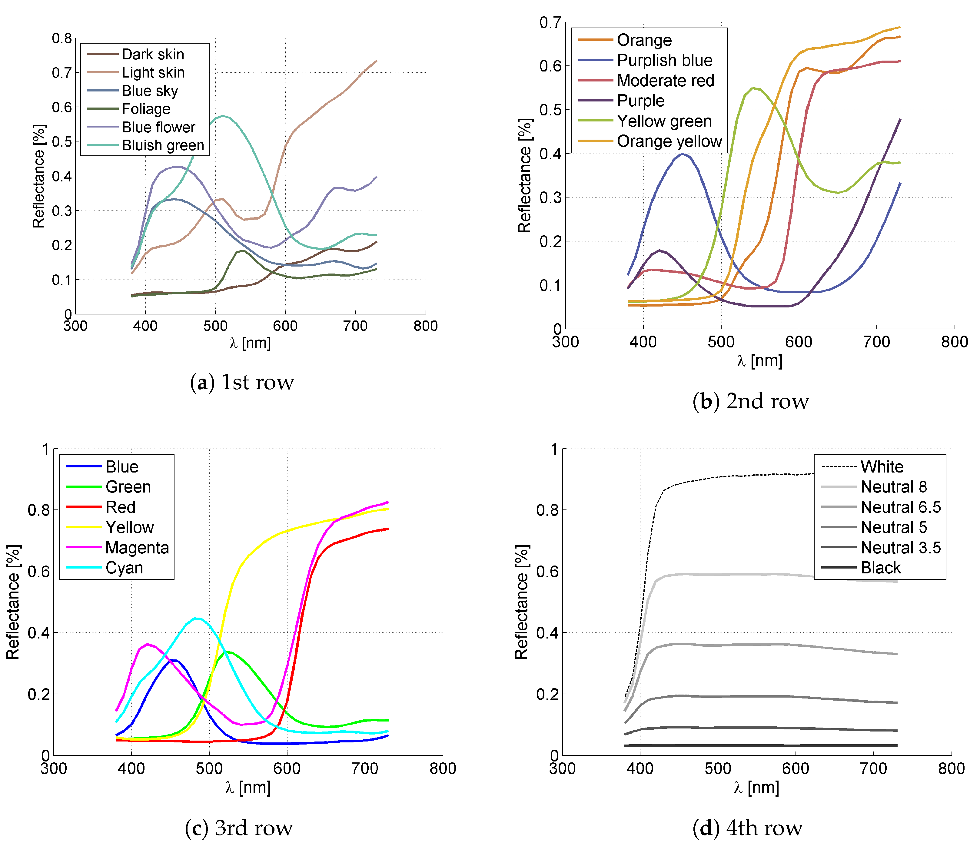
| ANN | McBeth spectral reflectance curves (Figure 8) |
| PCA [15] | none |
| CMF [18] | Stretched CIE 1964 color matching functions |
| CML [25] | Geographically-matched RGB image (Figure 1) |
| DHV [21] | none |
© 2020 by the authors. Licensee MDPI, Basel, Switzerland. This article is an open access article distributed under the terms and conditions of the Creative Commons Attribution (CC BY) license (http://creativecommons.org/licenses/by/4.0/).
Share and Cite
Coliban, R.-M.; Marincaş, M.; Hatfaludi, C.; Ivanovici, M. Linear and Non-Linear Models for Remotely-Sensed Hyperspectral Image Visualization. Remote Sens. 2020, 12, 2479. https://doi.org/10.3390/rs12152479
Coliban R-M, Marincaş M, Hatfaludi C, Ivanovici M. Linear and Non-Linear Models for Remotely-Sensed Hyperspectral Image Visualization. Remote Sensing. 2020; 12(15):2479. https://doi.org/10.3390/rs12152479
Chicago/Turabian StyleColiban, Radu-Mihai, Maria Marincaş, Cosmin Hatfaludi, and Mihai Ivanovici. 2020. "Linear and Non-Linear Models for Remotely-Sensed Hyperspectral Image Visualization" Remote Sensing 12, no. 15: 2479. https://doi.org/10.3390/rs12152479