Article

GIS-Based Machine Learning Algorithms for Gully Erosion Susceptibility Mapping in a Semi-Arid Region of Iran

1
College of Geology & Environment, Xi’an University of Science and Technology, Xi’an 710054, China
2
Key Laboratory of Coal Resources Exploration and Comprehensive Utilization, Ministry of Natural Resources, Xi’an 710021, China
3
Department of Watershed Management Engineering and Sciences, Faculty of Natural Resources and Marine Science, Tarbiat Modares University, Tehran 14115-111, Iran
4
Department of Watershed & Arid Zone Management, Gorgan University of Agricultural Sciences & Natural Resources, Gorgan 49189-434, Iran
5
Department of remote sensing and GIS, University of Tabriz, Tabriz 5166616471, Iran
6
Research Institute of the University of Bucharest, 90-92 Sos. Panduri, 5th District, Bucharest 013686, Romania
7
National Institute of Hydrology and Water Management, București-Ploiești Road, 97E, 1st District, Bucharest 013686, Romania
8
Department of Geomorphology, Faculty of Natural Resources, University of Kurdistan, Sanandaj 66177-15175, Iran
9
Board Member of Department of Zrebar Lake Environmental Research, Kurdistan Studies Institute, University of Kurdistan, Sanandaj 66177-15175, Iran
10
Department of Rangeland and Watershed Management, Faculty of Natural Resources, University of Kurdistan, Sanandaj 66177-15175, Iran
11
Institute of Research and Development, Duy Tan University, Da Nang 550000, Viet Nam
*
Author to whom correspondence should be addressed.
Remote Sens. 2020, 12(15), 2478; https://doi.org/10.3390/rs12152478
Submission received: 23 June 2020 / Revised: 26 July 2020 / Accepted: 29 July 2020 / Published: 2 August 2020

Abstract

:
In the present study, gully erosion susceptibility was evaluated for the area of the Robat Turk Watershed in Iran. The assessment of gully erosion susceptibility was performed using four state-of-the-art data mining techniques: random forest (RF), credal decision trees (CDTree), kernel logistic regression (KLR), and best-first decision tree (BFTree). To the best of our knowledge, the KLR and CDTree algorithms have been rarely applied to gully erosion modeling. In the first step, from the 242 gully erosion locations that were identified, 70% (170 gullies) were selected as the training dataset, and the other 30% (72 gullies) were considered for the result validation process. In the next step, twelve gully erosion conditioning factors, including topographic, geomorphological, environmental, and hydrologic factors, were selected to estimate gully erosion susceptibility. The area under the ROC curve (AUC) was used to estimate the performance of the models. The results revealed that the RF model had the best performance (AUC = 0.893), followed by the KLR (AUC = 0.825), the CDTree (AUC = 0.808), and the BFTree (AUC = 0.789) models. Overall, the RF model performed significantly better than the others, which may support the application of this method to a transferable susceptibility model in other areas. Therefore, we suggest using the RF, KLR, and CDT models for gully erosion susceptibility mapping in other prone areas to assess their reproducibility.

1. Introduction

Given the harmful effects of gully erosion, strategies for managing and reducing the damage caused by this phenomenon are essential to achieve sustainable development [1]. One of the strategies to achieve this goal is the use of gully erosion susceptibility mapping (GESM) [2]. This is well-known as an essential technique to address the mechanisms of gully erosion. To establish GESM, inventory maps of gully erosion and the methods for measuring the conditioning factors of gully erosion are needed [3]. A gully erosion susceptibility map can be constructed in the GIS environment by considering a set of variables that influence this phenomenon. A detailed analysis of the spatial correlation between these factors and the presence of gully erosion phenomena could also lead to a better estimation of gully erosion susceptibility [4]. Therefore, factors such as climate conditions, topography, geology, soil characteristics, and vegetation have a significant impact on the occurrence of gully erosion [5].
During the last few years, there has been a significant development in the application of machine learning algorithms in natural hazard studies, including floods [6,7,8], wildfire [9], sinkholes [10], drought [11,12], earthquakes [13,14], land subsidence [15,16], groundwater [17,18,19], landslides [20,21,22,23,24,25,26], and gullies [27,28,29,30,31]. Artificial intelligence is considered an advanced technique for predicting gully erosion, as well as managing and reducing the damage caused by this phenomenon. Indeed, Conoscenti et al. [32] assessed the gully erosion susceptibility in Sicily (Italy) using the logistic regression technique. An excellent discriminating ability was confirmed for gully erosion susceptibility with an area under the curve (AUC) greater than 0.8. In another study, Pourghasemi et al. [33] developed an ensemble model of an artificial neural network (ANN) and support vector machine (SVM) for gully erosion susceptibility mapping with promising results (i.e., AUCtrain = 0.897 and AUCtest = 0.879). Finally, the spatial occurrence pattern of gully erosion was properly addressed based on the developed models. Using different machine learning models, Rahmati et al. [34] also predicted and mapped the susceptibility of gully erosion with high performance. The random forest (RF) and RBF-SVM (radial basis function–SVM) models ultimately provided the highest accuracy and stability over other models. A similar study was also implemented for the same purposes based on the Naïve-Bayes tree (NBTree), Logistic Model Tree (LMT), and Alternating Decision Tree (ADTree) models. The findings indicated that the LMT model provided better performance than that of the ADTree and NBTree models. Conoscenti et al. [35] also applied the multivariate adaptive regression splines model to assess gully erosion susceptibility in Italy. Hydrological connectivity was investigated in their study to forecast gully erosion. Similar studies were likewise conducted and presented in [36,37,38,39,40,41,42].
Although gully erosion susceptibility has been studied and predicted by different machine learning algorithms and their accuracy has also been confirmed, these algorithms have not been applied in all areas. Meanwhile, the effects and levels of gully erosion in each region are different [43]. In the present study, gully erosion in the Markazi province (Iran), which has an arid and semi-arid climate, was investigated and predicted. Gullies often occur in this area and cause very extensive damage to the surrounding environment, as well as agriculture productivity [30,31]. Gullies are thus considered a major environmental problem that needs to be controlled and accurately predicted. The efforts of this study aim to establish a gully erosion map and evaluate the gully erosion susceptibility in the Robat Turk watershed in the west of Iran. The study area has an arid and semi-arid climate where various erosions have occurred in recent years, especially gully erosion; therefore, it is very important to study and evaluate this type of erosion in this area.
In the present study, we used four state-of-the-art machine learning models for predicting the gully erosion susceptibility in the Robat Turk Watershed of Iran: kernel logistic regression (KLR), best-first decision tree (BFTree), credal decision tree (CDTree), and random forest (RF). The novelty of this study is its use of the two algorithms, KLR and CDT, to evaluate gully erosion susceptibility in a semi-arid region. Although these two learning algorithms were previously suggested for and applied to landslide susceptibility mapping [44,45,46], flood susceptibility mapping [47], and groundwater potential mapping [48] across the world, they have been rarely applied to gully erosion modeling. Therefore, the ultimate aim of this study is to obtain accurate and reliable gully erosion susceptibility maps using some of the most advanced state-of-the-art machine learning algorithms.

2. Study Area and Dataset Preparation
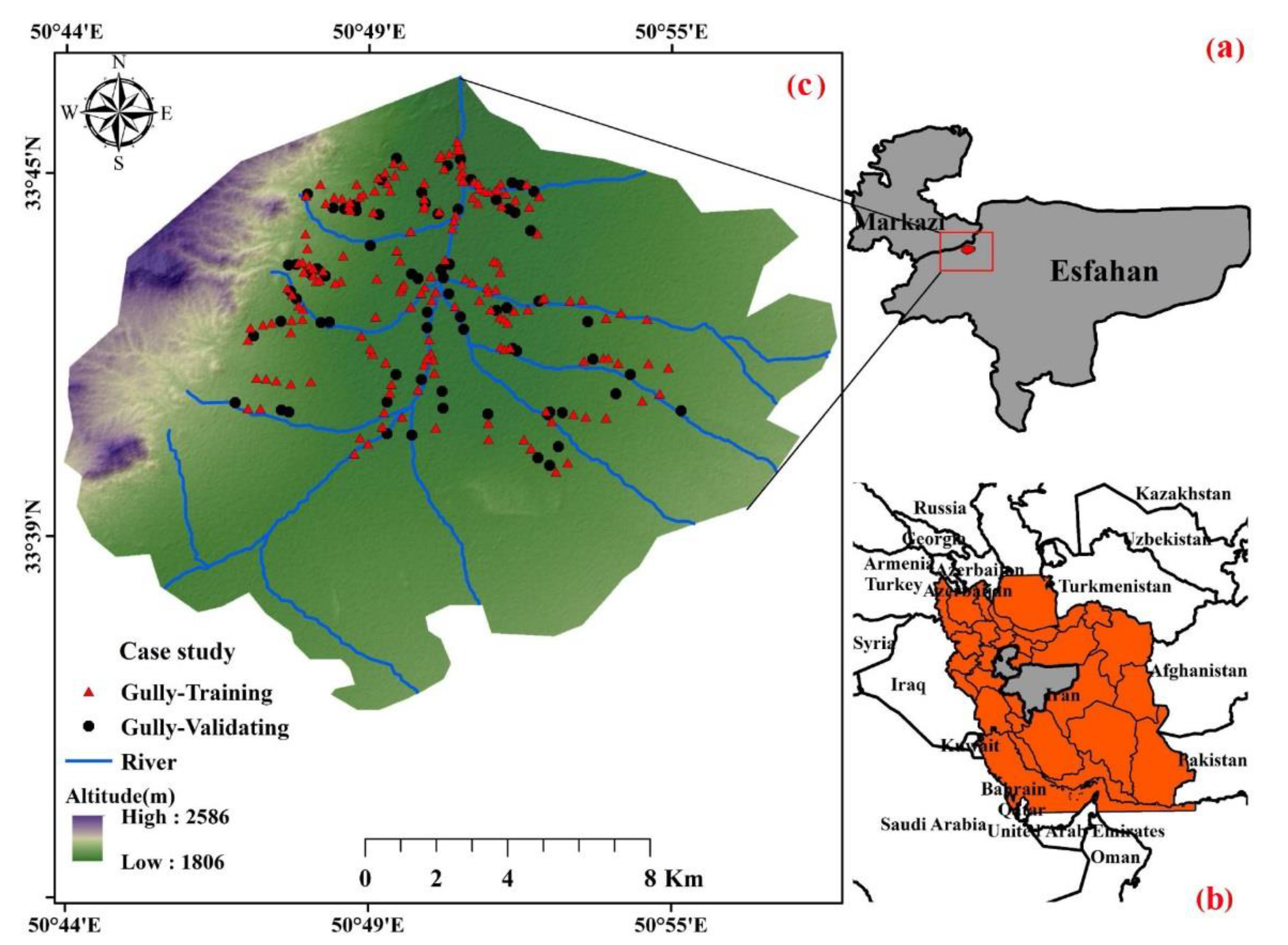
2.1. Study Area

The geographic coordinates of the Robat Turk Watershed are 33°35′ to 33°47′N latitude, 50°46′ to 50°52′E longitude, with an area of 242 km2, located between Makazi and Isfahan provinces (Figure 1). The Robat Turk has an arid and semi-arid climate, and the mean annual rainfall total is about 213 mm; most precipitation in the area occurs from winter to early spring (December to April) (Water Resources Company of Markazi 2017). The highest amount of runoff in the study area occurs from February to June [39]. In the Robat Turk watershed, there are both plain and mountainous units, and the formation of this area is largely composed of quaternary sediments. The oldest Precambrian metamorphic rocks (i.e., phyllite and quartzite), the Kahar Formation (i.e., shale, sandstone, and dolomite), and the Qom Formation can be observed in this area, along with alluvial units of the fourth period [49]. The catchment area indicates the presence of mountains, hills, and fluvial reliefs.
In terms of land use, most of the study area is surrounded by bare land areas (76%); however, the area has a poor range (18%) and agriculture (6%) units. As most of the area is covered by bare land areas, and the geological materials of these areas are mainly composed of young alluvium and river deposits, these areas are highly sensitive to soil erosion; despite having the least rainfall, the area’s water flow is concentrated and can induce rill erosion. With the development of the erodibility processes, these rill erosions become gully erosions in the study area, especially around the waterways where water infiltration is greater.

2.2. Gully Erosion Inventory Map

Extensive field surveys have conducted within the Robat Turk, and 242 gully erosion locations have recorded using a Global Positioning System (GPS; 76 CSX Garmin model) (Figure 1 and Figure 2). In each land use, the morphometric characteristics of the gullies, including the top width, down width, depth, and cross-sectional shape of the gullies, are different from each other. In agricultural land use, the average top width, down width, length, and depth of the gullies are 1073, 273, 304, and 5497 cm, respectively, and in rangeland use, the average high width, low width, length, and depth of the ditches are 993, 272, 273, and 3883 cm, respectively. A survey of the ratio of width to depth showed that in the agricultural land use areas, this ratio is equal to 2.40, and under rangeland land use, it is 2.23. The cross-sectional area is V-shaped in the agricultural land use unit and U-shaped under rangeland land use. In the agricultural land use unit, to a certain extent, several gullies are more active than the rangeland land use gullies. A survey of the morphometric characteristics of the gullies in the two land-use units show that in both land uses, the gullies are relatively active, and the shapes of their heads are concave and vertical. The presence of soil fragments inside the gully channel due to the collapse of the walls has caused the longitudinal profile to become convex in some cases; moreover, the transverse profiles of each gully are very different from each other.

2.3. Gully Erosion Conditioning Factors

There are many conditioning factors related to gully erosion, such as the rainfall erosion rate and the soil erosion rate. Therefore, a series of geographical, geological, and environmental characteristics should be understood when studying the process of gully erosion [50]. In the first step, a spatial database of gully erosion was established. The recorded gully erosion locations were randomly divided into a training dataset (70%) and a validation dataset (30%) [4,51,52]. Previous studies [31,53], using reliable data, identified the factors that affect the occurrence of gully erosion. Twelve factors were selected, including altitude, aspect, slope, plan curvature, profile curvature, normalized difference vegetation index (NDVI), distance from the river, drainage density, distance from the road, lithology, land use, and annual mean rainfall. We explain these conditioning factors and their effect on gully erosion as follows.
Altitude affects the types of vegetation and climate in a region. Therefore, many researchers believe that altitude plays a crucial role in the study of gully erosion [54]. The spatial resolution of the ALOS (advanced land observing satellite) PALSAR-DEM (the Phased-Array L-Band Synthetic Aperture Radar—Digital Elevation Model) is 12.5 m × 12.5 m (downloaded from https://vertex.daac.asf.alaska.edu). Previous studies have also shown that gully erosion is more likely to occur in low altitude areas [55,56] (Figure 3a).
In the investigation of environmental hazards and the development of susceptibility maps, aspect has a great influence [57]. Aspect, viewed through weathering mechanisms and the geomorphologic process, has an impact on gully erosion [58,59]. The aspect map for this study was extracted from the ALOS PALSAR-DEM and classified into nine classes, including flat, north, northeast, east, southeast, south, southwest, west, and northwest (Figure 3b).
The slope factor is strongly correlated with the amount of runoff and the soil erosion rate in an area [60]. Areas with low slopes are exposed to gully erosion via the accumulation of water flow [1,61]. This map was prepared in ArcGIS 10.2 using ALOS PALSAR-DEM and classified into five classes, including 0–5, 5–12, 12–20, 20–30, and >30 degrees (Figure 3c).
Water movement on the hillslopes is affected by the shape of the slope and causes changes in the amount of erosion [62,63]. The ALOS PALSAR-DEM was also used to provide the plan and profile curvatures, which were divided into three categories in ArcGIS 10.2 (Figure 3d,e).
The NDVI is very good for displaying vegetation biomass, leaf area index, crop yield, and vegetation separation and is also used for vegetation related issues [64]. This layer can also be effective in gully erosion modeling [33,65]. The NDVI map was provided using Landsat 8 data from 23/06/2017 (Figure 3f). The value of this factor can be obtained through the following formula:
N D V I =   N I R ( B a n d 4 ) R e d ( B a n d 3 ) N I R ( B a n d 4 ) + R e d ( B a n d 3 )
where Red represents the spectral reflectance value of red, and NIR represents the spectral reflectance value of the near-infrared band. The NDVI ranges from 1 to −1 [66].
The gully erosion locations are associated with a drainage network that facilitates the discharge of erosion from the upper reaches of the area [67]. Distance from the river layer was used to understand the effect of the drainage network on gully erosion [60]. The distance from the river was obtained using the Euclidean distance tool in ArcGIS 10.2 (Figure 3g). Drainage density has a direct relation to the amount of runoff in a catchment area [68]. This factor has a certain influence on the drainage pattern of an area, which depends on different factors, including geological formation, infiltration, soil characteristics, land use conditions, and slope [69,70]. The ArcGIS 10.2 software and line density tools were used to prepare the drainage density layer (Figure 3h).
Some phenomena, such as man-made roads and canals, have a profound effect on the occurrence of gully erosion [67,71,72]. Improper roads in bare lands could cause severe gully erosion [29]. A map of the distance from the road using a road network was constructed by the National Cartographic Center of Iran (INCC) at a scale of 1:25,000 in the ArcGIS 10.2 software (Figure 3i).
Another factor affecting the gully erosion analysis is lithology [73]. Lithological features are related to geomorphologic features and land surface characteristics [74]. Lithology unit maps were generated using a 1:100,000 scale geological map (GSI, 1997) from the Geological Survey and Mineral Exploration of Iran. The lithological map of the Robat Turk area was divided into eight classes (Figure 3j).
In recent decades, geological environments have been increasingly affected by human engineering activities, including oil and gas development [75] and transportation facility construction [76,77,78,79]. The interaction between land-use change and soil erosion has had an important impact on soil erosion and sediment production and has become a major environmental issue [56]. The landsat8 OLI image was downloaded from a web page (https://earthexplorer.usgs.gov/site) to produce the land use map. Then, pre-processing of the images, including geometric and radiometric corrections on the images, was performed in the ENVI 5.3 software to accurately observe the land use in the study area. Then, a false-color image was created for each image to better identify the land use in the area. To survey the land-use changes with a supervised method, land use maps obtained from the Department of Natural Resources of the Markazi Province along with field surveys and Google Earth were used to record numerous training samples for each land use. The maximum likelihood classifier was used to classify the training samples. The identified land uses in the region include bare land, rangeland, and agriculture areas (Figure 3k).
Rainfall acts as a triggering factor and penetrates the cracks in the soil, causing an expansion of the gully in different directions [51]. In this study, the rainfall layer was obtained using three rainfall stations inside and outside the study watershed (from the Markazi County Meteorological Bureau). Different interpolation methods were used to detect the target layer; then, the inverse distance weighting (IDW) interpolation method was used to draw the total annual rainfall map, thereby improving the accuracy [80,81,82].

3. Methods

The methodological workflow to derive the final gully erosion susceptibility map is shown in Figure 4.

3.1. Multicollinearity Analysis

In natural event studies, multicollinearity points to the lack of independence of the independent variables and their strong associations, which can occur in a dataset due to their high correlation and thus confuse an analysis of their incidence [83]. Variance inflation factors (VIFs) and tolerance (TOL) [84] can determine the relationship between factors. In the present study, the TOL and VIF are used to study the multicollinearity of independent variables in gully erosion modeling [33,85]. If the VIF is higher than 10 and the TOL value is less than 0.1, then the multi-collinearity among the variables is error-prone [84].

3.2. Background of the Data Mining Models

3.2.1. Kernel Logistic Regression (KLR)

KLR is a powerful classification technique compared to other traditional classification methods [66]. This model has been successfully used in many of the classified problems [86]. Although KLR can transfer indivisible linear problems, it uses the core to transfer input features to the next space of higher dimensions, but this is not possible for the LR model [87]. The advantages of the KLR learning algorithm include its ability to predict an event according to its probability and its capacity to be extended to multi-class classification problems [88,89]. KLR is known to be a powerful classifier [90]. However, KLR is not sparse and requires all training instances in its model [91]. KLR can intrinsically provide probabilities and straightforwardly develop multi-class classification problems that only require solving an unconstrained quadratic program [45]. Specifically, when the optimization algorithm is suitable, as the algorithm does not need to solve the quadratic equation, it can perform analysis more quickly than other algorithms such as SVM [45,92]. To apply this model, the statistical software R (version 3.5.2) was used.

3.2.2. Credal Decision Trees (CDTree)

The main feature of decision trees is their internal inconsistency; even with a set of different training datasets related to a particular issue, various decision trees will be created. This feature is an essential feature that makes decision trees an appropriate classifier in ensemble models, such as bagging, boosting, and random forest. In this method, like in the classic decision tree technique, every node represents a variable property, and every branch illustrates one of the conditions of this factor [93].
A leaf node is formed when it arrives at a factor and does not provide more information about the factor class; the information is thus based on uncertainty through measurement (the measurement of maximum entropy), and more factors are not entered. The leaf node, which is the predicted value based on the information in the dataset class variable, defines the model’s training. When the decision tree is created, a new instance of the X test set is used in the decision tree. For example, after the cases of the X-property variables in the decision tree, the root node is set to a leaf node. Finally, the value of the leaf node is obtained by classifying the X class through a credal decision tree [93]. The advantage of the CDT algorithm is that it offers good experimental results [94,95] and it is especially suitable when noisy data are classified [96]. The disadvantage of CDT is that it only defines discrete variables, does not work with missing values, and does not engage in a posterior pruning process [97].

3.2.3. Random Forest (RF)

RF is one of the most widely used algorithms due to its simplicity and capabilities [98,99,100]. This algorithm generates a forest randomly; this “forest” is a group of decision trees. The construction of a forest using trees is often done via the “bagging” method [101]. The main concept of the bagging method is that combining multiple models will produce better results than a single model. Simply put, a random forest is composed of a set of decision trees; this combination is not only used to make the prediction more accurate but also to make it more sustainable. The advantage of the random forest method is that it can reduce both oscillations and the evaluation of variance [102]. After fully building the trees, the test data are introduced into the tree, and the tree number is obtained for the input vector of an output. Using the average of these outputs, the final output of the model and the empirical distribution of the outputs are calculated by the percentage value and the range of uncertainty. The random regression tree method is a proven method, especially when the number of observations relative to the predictor is small [103].
The node size variable (which represents the number of leaves per branch) was determined in this study by trial and error. The random forest adds random branches to the model as the trees grow. Instead of looking for the most important feature when dividing a node, this model searches for the most important feature among a set of random features. This leads to too many variations and, ultimately, a better model [62,101,104].

3.2.4. Best-First Decision Tree (BFTree)

Ensemble-learning models, or data mining techniques, can specifically consider multiple classifications in the best-first decision tree and determine the importance of each classifier [105]. Prenatal options are available before and after finding the best number of extensions for application through cross-validation in the training data. Although these trees can be fully developed in the same manner regardless of the first algorithm or the first depth, the BFTree uses different pruning modes generated by the first depth method [106]. Another BFTree-based classification algorithm involves the creation of a functional tree with diagonal splits and linear functions in the leaf [107].

3.3. Evaluation of the Model Performance

3.3.1. Statistical Measures

Although various studies used different methods to evaluate data mining models, we employed the most important measures that have been used by the majority of environmental researchers. In this study, the performance of these models will be evaluated through the following statistical measures: sensitivity, specificity, and accuracy. The following relationships are used to obtain statistical measures [108,109]:
S e n s i t i v i t y = T P T P + F N
S p e c i f i c i t y = T N F P + T N
A c c u r a c y = T P + T N T P + F P + T N + F N
where TP (true positive) and TN (true negative) are correctly classified pixels, and FP (false positive) and FN (false negative) are the incorrectly classified pixels.

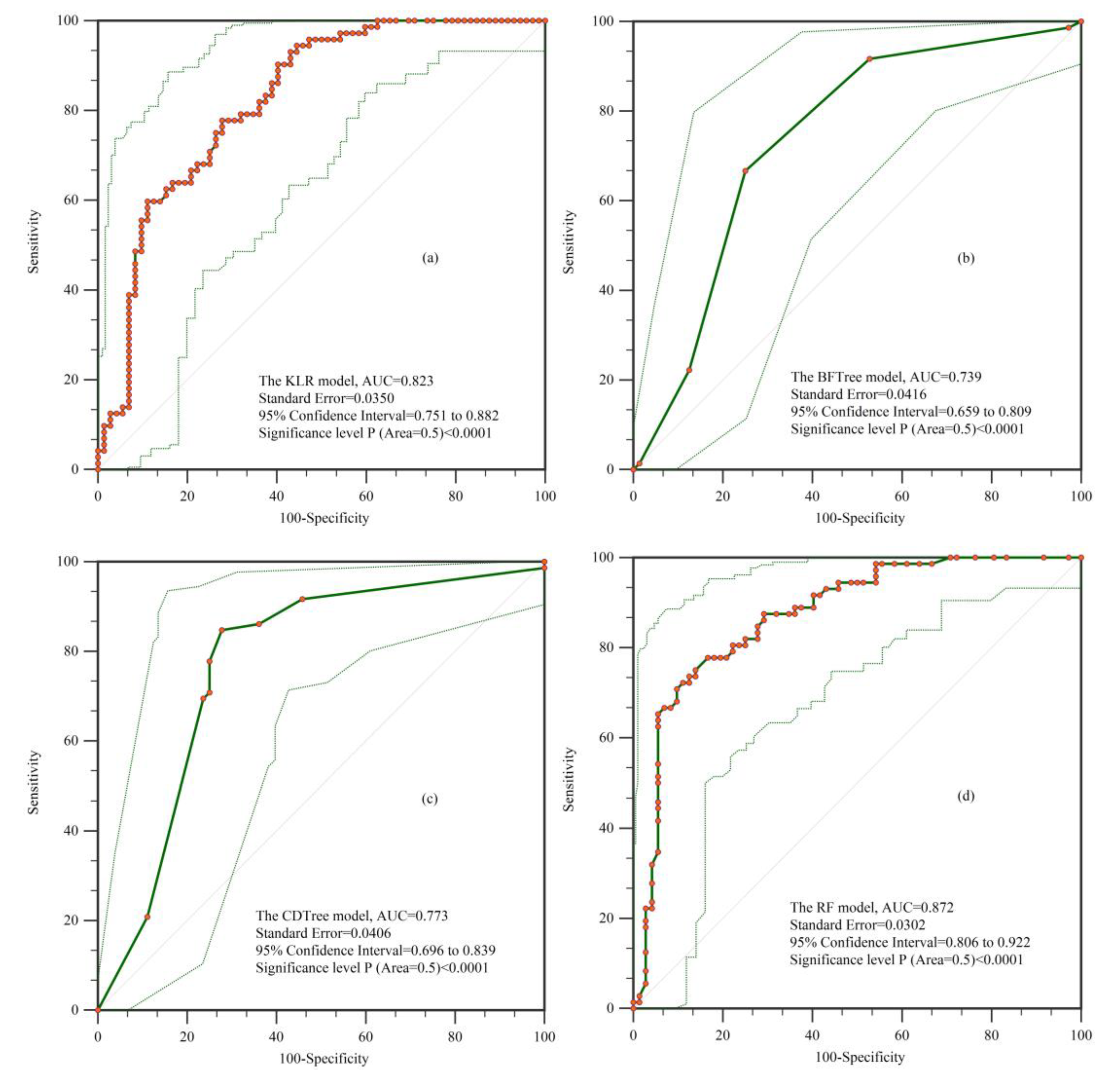
3.3.2. ROC Curve and AUC

The results were validated with the help of the receiver operating characteristic (ROC) curves [18,73,110]. The ROC curve is plotted based on a 1- specificity (x-axis) against sensitivity (y-axis) [111,112]. The area under the ROC curve (AUC) represents the ability to model whether the predetermined event will occur [113,114]. The closer the AUC value is to 1, the higher the accuracy of the results will be [115]. The AUC can be calculated by this formula [108]:
  AUC = ( T P + T N ) ( P + N )
where P and N represent the total number of pixels with and without gully erosion, respectively.

4. Results and Analysis

4.1. Assessing the Affecting Factors Using Multicollinearity Analysis

In this study, the frequency ratio method was used to study the relationship between each factor category and gully erosion point, and each factor category was given a specific weight [4,53]. The multicollinearity test was used to study the interrelationship among the impact factors, while mainly considering the VIF and TOL (Figure 5). The experimental results of the multicollinearity test assign the highest VIF values (5.329) to altitude, followed by land use (3.525) and distance from the river (2.875). However, the smallest TOLs were assigned to altitude and land use with values of 0.188 and 0.284, respectively. Overall, since the VIF values did not exceed the critical value of 10, and the TOL was lower than 0.1, there no multicollinearity problem was found among the gully erosion conditioning factors.

4.2. Configuration and Training of the Data Mining Models

Since there is no multicollinearity problem among the gully erosion conditioning factors, all 12 factors were used to train the four machine learning models. Reconfiguration of the model’s architecture achieved the goal of optimizing model performance. For the RF model, 100 iterations and 10-fold cross-validation offered the greatest prediction performance. For the CDTree model, the minimum total weight of the instances in a leaf was set as 2, and 10-fold cross-validation was used for pruning. For the KLR model, RBFKernel, a lambda value of 0.01, and a gamma value of 0.01 were used. For the BFTree model, the minimum number of instances at the terminal nodes was set to 2, the number of folds for internal cross-validation was set to 5, and post-pruning was adopted. After the configuration of the model was completed, training and verification were carried out, and the model was ultimately obtained.

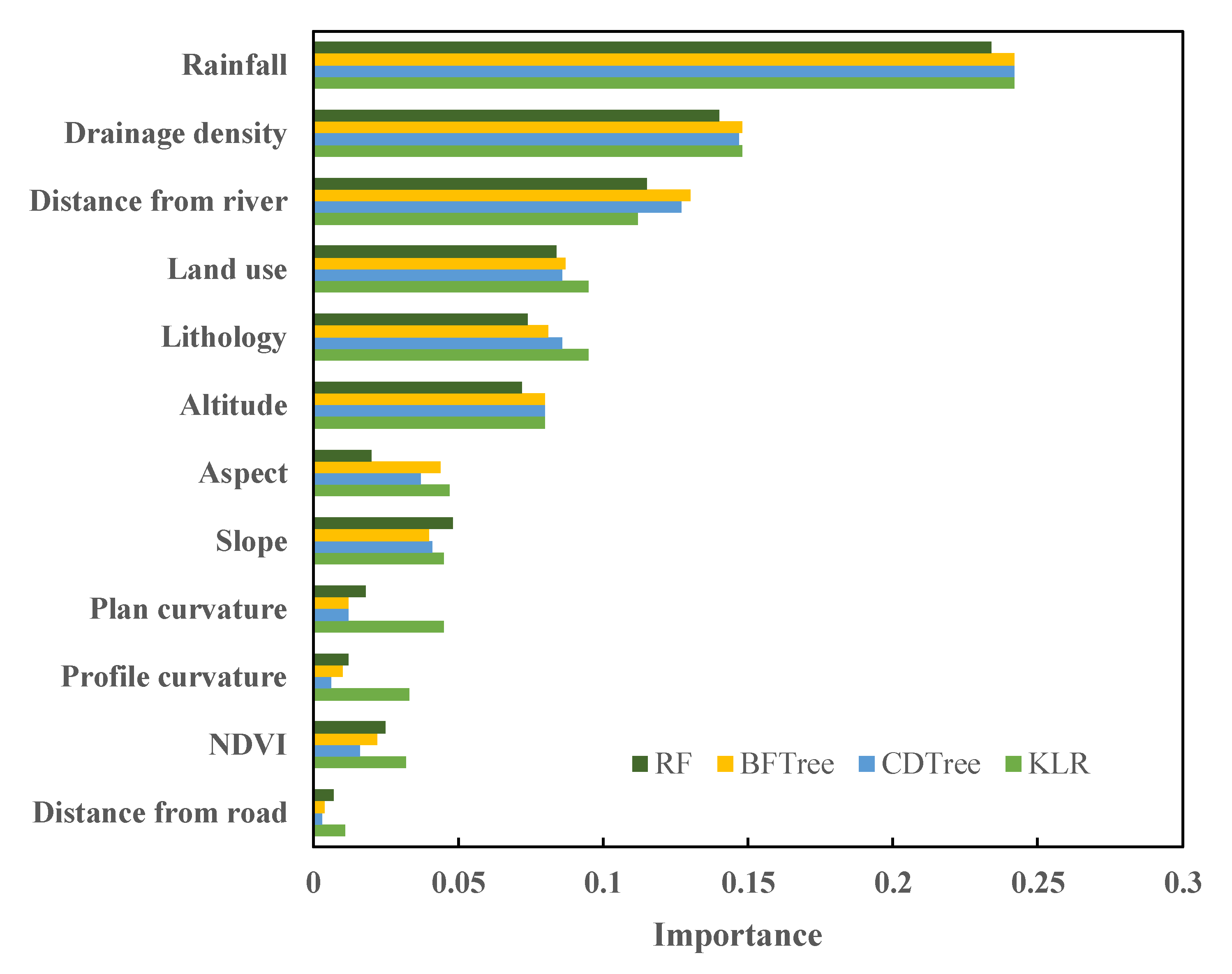
4.3. Variable Importance

The importance of each gully erosion conditioning factor is another mandatory output used to compute gully erosion susceptibility. The importance values for the 12 conditioning factors were thus considered for gully erosion susceptibility mapping. These values were automatically produced during the model training procedure of the different algorithms (Figure 6). For the KLR model, rainfall was the most important (0.242), followed by drainage density (0.148), distance from the river (0.112), lithology (0.095), and land use (0.095). For CDTree, the most important factor was also rainfall (0.242), followed by drainage density (0.147), distance from the river (0.127), land use (0.086), and lithology (0.086). The results provided by the BFTree algorithm showed that rainfall was again the most important factor (0.242), followed by drainage density (0.148), distance from the river (0.13), land use (0.087), and lithology (0.081). The RF model also indicated that rainfall was the most important gully erosion factor (0.234), followed by drainage density (0.14), distance from river (0.115), land use (0.084), and lithology (0.074). The results showed that the rainfall layer was the most important among the applied layers. Drainage density and distance from the river layers were also subsequently determined.

4.4. Model Performace Evaluation

The performance of the models was evaluated using the statistical measures for both the training and validating datasets. In terms of sensitivity, after using the training datasets, the best model was shown to be the RF (0.853) model, followed by the CDTree (0.847), BFTree (0.841), and KLR (0.794) models (Table 1). The specificity result showed that the best model was again RF (0.800), but this time the BFTree (0.706) ranked second, followed by the KLR (0.694) and CDTree (0.688) models. In terms of classification accuracy, the best model highlighted by the training dataset was the RF (0.826) model, followed by the BFTree (0.774), CDTree (0.768), and KLR (0.744) models. However, the sensitivity calculated using the validation dataset indicated that RF and CDTree (0.847) were more reliable models than the KLR (0.778) and BFTree (0.667) models. However, the BFTree model had the highest specificity (0.750), followed by the RF, CDTree, and KLR models (0.722). In terms of accuracy, the RF and CDTree models had higher values (0.785) compared to the KLR (0.750) and BFTree (0.708) models.
Overall, for all the statistical measures, the values were higher than 0.7. Therefore, all the models possess a strong ability to provide gully erosion susceptibility maps. However, the RF model has a more balanced performance with the training and validation datasets.
The ROC curve [116,117] was used to evaluate the accuracy of the GESM results, and the AUC was used to accurately quantify these models [66,118,119]. Figure 7 shows that the RF (AUC = 0.893) model has the best success rate curve based on the training dataset. Similarly, the RF model ranks first in its prediction rate (AUC = 0.872). According to the literature, the optimization levels of algorithms can be assessed based on the accuracy of their validation rates [120,121]. After comprehensively considering the AUC values of the four models shown in Figure 7 and Figure 8, the RF model was determined to be the most robust and effective.
As shown in Figure 8, the criterion of the standard error (SE) was also used to determine the accuracy rates of the validation dataset; these rates were the best for all four models and were 0.035, 0.041, 0.040, and 0.030 for the KLR, BFTree, CDTree, and RF models, respectively. The results of the confidence interval (CI) also confirmed that the RF model had the narrowest 95% confidence interval (0.806 to 0.922). Further, in conjunction with the results of the AUC, the results of the two other indicators, SE and CI, confirmed that the RF model was more accurate in predicting gully erosion susceptibility than the KLR, CDTree, and BFTree models.

4.5. Creating Susceptibility Maps Using the KLR, BFTree, CDTree, and RF models

To generate susceptibility maps of gully erosion, in the first stage, each raster representing the gully erosion predictors was multiplied with the related importance value achieved following the training process of the four data mining models. Then, using the map algebra function, the products resulting from the multiplication were summed to derive the final GESM across the study area.
Some classification methods are included in GIS, including natural breaks, quantile, geometric interval, equal interval, and standard deviation. We tested all these models, and the best one was found to be a natural break. The natural break method was thus used to divide the final mapping generated by these models into four categories [23,122]. This method was then used to classify the values of the gully erosion maps because, in this method, classes and classification are determined based on the inherent natural groupings in each group. A break in the class or the threshold of each class indicates that the effects of this group are most similar. On the other hand, these classes will have the greatest differences from each other. Indeed, the classes and tools that are most different from each other are separated and classified in a given situation [123,124]. The application of the KLR model revealed that high and very high susceptibility values were present throughout approximately 37.61% of the Robat Turk watershed (Figure 9a and Figure 10). In total, 61.98% of the research territory was included by the CDTree model in areas with a low gully susceptibility value. In this case, moderate values comprised around 6.20% of the study area, while high and very high susceptibility were spread throughout approximately 31.82% of the study area (Figure 9b and Figure 10). The BFTree model showed that areas with low gully erosion susceptibility were located in 53.31% of the Robat Turk watershed, while those with moderate values spanned over 21.9% (Figure 9c and Figure 10). The results of the RF model revealed that more than 47% of the study area belonged to an area with low susceptibility to gully erosion, while areas with moderate values occupied 19.01% (Figure 9d and Figure 10). Together, areas with high and very high gully erosion susceptibility covered more than 33% of the Robat Turk watershed. By analyzing the results provided by the susceptibility maps of gully erosion derived from the four algorithms, the low susceptibility class was found to occupy the largest area of Robat Turk.

5. Discussion

In the present study, the important variables affecting gully erosion in the Robat Turk watershed derived using data mining models showed that rainfall, altitude, distance from the river, and land use are more important than the other variables. This fact is largely in agreement with the results achieved by Rahmati et al. [4] and Tien Bui et al. [31], according to which the distance from rivers and land use are more important than other geographical variables. These results confirm that many more locations relevant to gully erosion exist in regions with more rainfall and low altitude values. Further, in areas with bare land, the concentration of gully erosion locations is greater. In other words, while most gullies occur on bare lands, lowland areas contain more gully erosion locations. This shows that bare lands cover the majority of the study area, which is characterized by a low altitude. This also indicates a significantly positive relationship between altitude and land use. Recently, evaluating the factors controlling gully erosion has been widely considered and discussed in the literature [1,34,85,125,126]. In general, altitude and land use are the most commonly reported influential factors [127,128]. In terms of factor importance, distance from the rivers ranked third in this study. Conoscenti et al. [32] noted that most of these gullies are connected to river networks in the area, which increases erosion from the upland area. The influence of land use on gully activity was also reported in Vandekerckhove et al. [127]; however, there are many doubts about the features that induce subsurface gully development. It was reported in Hosseinalizadeh et al. [125] that changes in land use and mismanagement practices play the main roles in establishing gully head cut landforms. The impact of land use on gully development was also reported by Vandekerckhove et al. [127], although there remains uncertainty about the variables inducing gully activity and their interactions with other subsurface processes. It has also been proven that gully rates are highly dependent on the size of the runoff-contributing region above the gully erosion [129].
Additionally, gully erosion is widespread and mitigates other types of soil erosion, such as wind erosion, in different ecosystems. Thus, it is necessary to predict and map gully susceptibility. Data mining methods are reliable tools for mitigating and controlling the influence of soil erosion in different regions all over the world. In the present study, this issue was addressed by comparing and analyzing four data mining models—KLR, BFTree, CDTree, and RF—by applying the twelve affecting factors. All four models showed their most susceptible regions to be located in the northern part of the study area, whereas approximately 51% of the area was specified in the low susceptibility class. The RF model had the greatest AUC of 0.872 for the validation dataset, as well as the smallest standard error and confidence interval. This is because the RF model manages both categorical and continuous data and does not prioritize any model dependencies [130]. Additionally, the RF model handles input data without data elimination, leading to high prediction accuracy [131]. This model has been used in various studies and is mostly reported to be an accurate model [132,133].
Conversely, the BFTree model had the smallest validation rate (AUC: 73.9%) among the three models tested in this area and thus cannot be suggested for use as an advanced technique for the statistical analysis of gully erosion. Based on these results, we conclude that the RF model has the greatest accuracy, while the lowest accuracy was obtained by the BFTree. A comparison between the applied methods and other ensemble models for the spatial distribution of gully erosion could be a primary aim in future studies.
Pham and Prakash [45] compared the efficiency of the KLR and classification and regression tree (CART) algorithms. The authors concluded that the KLR model outperformed and outclassed the CART model in shallow landslide susceptibility mapping at the tri-junction of the Rudrapryag, Tehri Garhwal, and Pauri Garhwal districts (Uttarakhand, Himalayas, India). Nguyen et al. [48] used the CDTree algorithm as a base classifier to construct five hybrid models: Bagging-CDTree, Dagging-CDTree, Decorate-CDTree, MultiBoost-CDTree, and Random Subspace-CDTree. These models were developed for and applied to the groundwater potential mapping of DakLak province in Vietnam. The authors revealed that the ensemble models can significantly improve the performance of the CDTree algorithm. In another study, Chen et al. [18] compared the KLR, RF, and ADT algorithms for groundwater potential mapping of the Ningtiaota region in the northern territory of Shaanxi Province, China. They noted that the RF model provided the highest AUC value (0.811) followed by the KLR (0.797) and ADTree (0.773) models. In a comparison between BFTree, RF, and naïve Bayes tree (NBTree), Chen et al. [134] evaluated their performance and revealed that the RF algorithm outperforms the BFTree and NBTree algorithms in landslide susceptibility mapping.
Recently, Bernatek-Jakiel and Wrońska-Wałach [135] determined that gullies initiate and develop in the regions that are most susceptible to piping erosion. Other scientists have observed that gullies indicate geomorphologic changes throughout the world [136,137]. These observations indicate that gullies are deepened and developed via subsurface processes, mostly at low altitudes [135]. Also, as reported recently by Hosseinalizadeh et al. [125], the positive interactions between collapsed pipes and gully head cuts are due to soil degradation processes. Based on the archived results, gullies are recognized as the main cause of the soil erosion and degradation processes in the study area, as well as the main initiator of the sediment movement delivered to the rivers. Additionally, because of the bare land covering the majority of the study area, the land without vegetation has a negative effect on the infrastructure of the area to be damaged. Thus, soil-erodibility factors can significantly increase due to a high rate of soil loss.

6. Conclusions

The development of gullies leads to wasteful amounts of soil. Therefore, gully erosion is an important cause of land and environmental degradation. This paper mainly studied the impact of different data mining models on compiling a susceptibility map of a gully. To do this, 12 important and influential factors on gully erosion and 242 gully erosion locations were used. For modeling, the CDTree, KLR, RF, and BFTree machine learning algorithms were used. The results for the effectiveness of the AUC-based models in mapping gully erosion susceptibility showed that the RF model offers the highest efficiency, while the BFTree model has lower performance than the other two models. Reducing the destructive impact of this type of erosion and preventing its deterioration is a problem that needs to be resolved urgently, as it is necessary to identify this type of erosion. Since most gullies are located in the central part of the study area near the village of Robat Turk, the protective practices in these areas must be increased, and the extension of agriculture and residential areas to areas of deterioration should be prevented. Using data mining methods in other study areas by identifying the geological conditions and geo-environmental factors affecting gully erosion could be used to save time and costs when mapping the susceptibility of erosion.
Studies also showed that susceptibility maps can effectively help select various mitigation options [138]. Land use planning or urban construction could be carried out in low gully-prone areas, which could effectively reduce the losses caused by environmental hazards [139]. Susceptibility maps are of great significance; most notably, the rational use of these maps in the planning stage can yield large benefits. As a result, the proposed methods and corresponding susceptibility maps could aid local governments and related organizations in pursuing new and existing spatial planning projects, thereby taking effective measures to achieve disaster reduction and loss reduction [140].
Therefore, we suggest using the RF, KLR, and the CDT models for gully erosion susceptibility mapping in other prone areas to check their reproducibility. The results of this study provide beneficial insights for sustainable development strategies and minimizing destructive hazards to the surrounding environment via gully erosion susceptibility mapping.

Author Contributions

X.L., W.C., M.A., S.J., N.K., H.S. (Hejar Shahabi), R.C., H.S. (Himan Shahabi), A.S., and A.M. contributed equally to this work. M.A., S.J., N.K., and H.S. (Hejar Shahabi) collected field data. X.L., W.C., M.A., S.J., N.K., and H.S. (Hejar Shahabi) conducted the modeling and wrote the manuscript. W.C., R.C., H.S. (Himan Shahabi), A.S., and A.M. provided critical comments in the planning of this paper and edited the manuscript. X.L., W.C., R.C., H.S. (Himan Shahabi), A.S., and A.M. contributed to the revision of the manuscript. All authors discussed the results and edited the manuscript. All authors have read and agreed to the published version of the manuscript.

Funding

This study was supported by the Innovation Capability Support Program of Shaanxi (Program No. 2020KJXX-005).

Conflicts of Interest

The authors declare no conflict of interest.

References

  1. Valentin, C.; Poesen, J.; Li, Y. Gully erosion: Impacts, factors and control. Catena 2005, 63, 132–153. [Google Scholar] [CrossRef]
  2. Arabameri, A.; Blaschke, T.; Pradhan, B.; Pourghasemi, H.R.; Tiefenbacher, J.P.; Bui, D.T. Evaluation of recent advanced soft computing techniques for gully erosion susceptibility mapping: A comparative study. Sensors 2020, 20, 335. [Google Scholar] [CrossRef] [Green Version]
  3. Gayen, A.; Pourghasemi, H.R.; Saha, S.; Keesstra, S.; Bai, S. Gully erosion susceptibility assessment and management of hazard-prone areas in india using different machine learning algorithms. Sci. Total Environ. 2019, 668, 124–138. [Google Scholar] [CrossRef]
  4. Rahmati, O.; Haghizadeh, A.; Pourghasemi, H.R.; Noormohamadi, F. Gully erosion susceptibility mapping: The role of gis-based bivariate statistical models and their comparison. Nat. Hazards 2016, 82, 1231–1258. [Google Scholar] [CrossRef]
  5. Conforti, M.; Aucelli, P.P.; Robustelli, G.; Scarciglia, F. Geomorphology and gis analysis for mapping gully erosion susceptibility in the turbolo stream catchment (northern calabria, italy). Nat. Hazards 2011, 56, 881–898. [Google Scholar] [CrossRef]
  6. Wang, Y.; Hong, H.; Chen, W.; Li, S.; Panahi, M.; Khosravi, K.; Shirzadi, A.; Shahabi, H.; Panahi, S.; Costache, R. Flood susceptibility mapping in dingnan county (china) using adaptive neuro-fuzzy inference system with biogeography based optimization and imperialistic competitive algorithm. J. Environ. Manag. 2019, 247, 712–729. [Google Scholar] [CrossRef]
  7. Shahabi, H.; Shirzadi, A.; Ghaderi, K.; Omidvar, E.; Al-Ansari, N.; Clague, J.J.; Geertsema, M.; Khosravi, K.; Amini, A.; Bahrami, S. Flood detection and susceptibility mapping using sentinel-1 remote sensing data and a machine learning approach: Hybrid intelligence of bagging ensemble based on k-nearest neighbor classifier. Remote Sens. 2020, 12, 266. [Google Scholar] [CrossRef] [Green Version]
  8. Chen, W.; Li, Y.; Xue, W.; Shahabi, H.; Li, S.; Hong, H.; Wang, X.; Bian, H.; Zhang, S.; Pradhan, B. Modeling flood susceptibility using data-driven approaches of naïve bayes tree, alternating decision tree, and random forest methods. Sci. Total Environ. 2020, 701, 134979. [Google Scholar] [CrossRef] [PubMed]
  9. Jaafari, A.; Zenner, E.K.; Panahi, M.; Shahabi, H. Hybrid artificial intelligence models based on a neuro-fuzzy system and metaheuristic optimization algorithms for spatial prediction of wildfire probability. Agric. For. Meteorol. 2019, 266, 198–207. [Google Scholar] [CrossRef]
  10. Taheri, K.; Shahabi, H.; Chapi, K.; Shirzadi, A.; Gutiérrez, F.; Khosravi, K. Sinkhole susceptibility mapping: A comparison between bayes-based machine learning algorithms. Land Degrad. Dev. 2019, 30, 730–745. [Google Scholar] [CrossRef]
  11. Roodposhti, M.S.; Safarrad, T.; Shahabi, H. Drought sensitivity mapping using two one-class support vector machine algorithms. Atmos. Res. 2017, 193, 73–82. [Google Scholar] [CrossRef]
  12. Choubin, B.; Soleimani, F.; Pirnia, A.; Sajedi-Hosseini, F.; Alilou, H.; Rahmati, O.; Melesse, A.M.; Singh, V.P.; Shahabi, H. Effects of drought on vegetative cover changes: Investigating spatiotemporal patterns. In Extreme Hydrology and Climate Variability; Elsevier: Amsterdam, The Netherlands, 2019; pp. 213–222. [Google Scholar]
  13. Lee, S.; Panahi, M.; Pourghasemi, H.R.; Shahabi, H.; Alizadeh, M.; Shirzadi, A.; Khosravi, K.; Melesse, A.M.; Yekrangnia, M.; Rezaie, F. Sevucas: A novel gis-based machine learning software for seismic vulnerability assessment. Appl. Sci. 2019, 9, 3495. [Google Scholar] [CrossRef] [Green Version]
  14. Alizadeh, M.; Alizadeh, E.; Kotenaee, S.A.; Shahabi, H.; Pour, A.B.; Panahi, M.; Ahmad, B.B.; Saro, L. Social vulnerability assessment using artificial neural network (ann) model for earthquake hazard in tabriz city, iran. Sustainability 2018, 10, 3376. [Google Scholar] [CrossRef] [Green Version]
  15. Bui, D.T.; Shahabi, H.; Shirzadi, A.; Chapi, K.; Pradhan, B.; Chen, W.; Khosravi, K.; Panahi, M.; Ahmad, B.B.; Saro, L.J.S. Land subsidence susceptibility mapping in south korea using machine learning algorithms. Sensors 2018, 18, 2464. [Google Scholar]
  16. Rahmati, O.; Samadi, M.; Shahabi, H.; Azareh, A.; Rafiei-Sardooi, E.; Alilou, H.; Melesse, A.M.; Pradhan, B.; Chapi, K.; Shirzadi, A. Swpt: An automated gis-based tool for prioritization of sub-watersheds based on morphometric and topo-hydrological factors. Geosci. Front. 2019, 10, 2167–2175. [Google Scholar] [CrossRef]
  17. Rahmati, O.; Naghibi, S.A.; Shahabi, H.; Bui, D.T.; Pradhan, B.; Azareh, A.; Rafiei-Sardooi, E.; Samani, A.N.; Melesse, A.M. Groundwater spring potential modelling: Comprising the capability and robustness of three different modeling approaches. J. Hydrol. 2018, 565, 248–261. [Google Scholar] [CrossRef]
  18. Chen, W.; Li, Y.; Tsangaratos, P.; Shahabi, H.; Ilia, I.; Xue, W.; Bian, H. Groundwater spring potential mapping using artificial intelligence approach based on kernel logistic regression, random forest, and alternating decision tree models. Appl. Sci. 2020, 10, 425. [Google Scholar] [CrossRef] [Green Version]
  19. Nhu, V.-H.; Rahmati, O.; Falah, F.; Shojaei, S.; Al-Ansari, N.; Shahabi, H.; Shirzadi, A.; Górski, K.; Nguyen, H.; Ahmad, B.B. Mapping of groundwater spring potential in karst aquifer system using novel ensemble bivariate and multivariate models. Water 2020, 12, 985. [Google Scholar] [CrossRef] [Green Version]
  20. Bui, D.T.; Shahabi, H.; Omidvar, E.; Shirzadi, A.; Geertsema, M.; Clague, J.J.; Khosravi, K.; Pradhan, B.; Pham, B.T.; Chapi, K. Shallow landslide prediction using a novel hybrid functional machine learning algorithm. Remote Sens. 2019, 11, 931. [Google Scholar]
  21. Shirzadi, A.; Solaimani, K.; Roshan, M.H.; Kavian, A.; Chapi, K.; Shahabi, H.; Keesstra, S.; Ahmad, B.B.; Bui, D.T. Uncertainties of prediction accuracy in shallow landslide modeling: Sample size and raster resolution. Catena 2019, 178, 172–188. [Google Scholar] [CrossRef]
  22. Shahabi, H.; Khezri, S.; Ahmad, B.B.; Hashim, M. Landslide susceptibility mapping at central zab basin, iran: A comparison between analytical hierarchy process, frequency ratio and logistic regression models. Catena 2014, 115, 55–70. [Google Scholar] [CrossRef]
  23. Zhao, X.; Chen, W. Gis-based evaluation of landslide susceptibility models using certainty factors and functional trees-based ensemble techniques. Appl. Sci. 2020, 10, 16. [Google Scholar] [CrossRef] [Green Version]
  24. Nhu, V.-H.; Mohammadi, A.; Shahabi, H.; Ahmad, B.B.; Al-Ansari, N.; Shirzadi, A.; Clague, J.J.; Jaafari, A.; Chen, W.; Nguyen, H. Landslide susceptibility mapping using machine learning algorithms and remote sensing data in a tropical environment. Int. J. Environ. Res. Public Health 2020, 17, 4933. [Google Scholar] [CrossRef] [PubMed]
  25. Nhu, V.-H.; Shirzadi, A.; Shahabi, H.; Singh, S.K.; Al-Ansari, N.; Clague, J.J.; Jaafari, A.; Chen, W.; Miraki, S.; Dou, J. Shallow landslide susceptibility mapping: A comparison between logistic model tree, logistic regression, naïve bayes tree, artificial neural network, and support vector machine algorithms. Int. J. Environ. Res. Public Health 2020, 17, 2749. [Google Scholar] [CrossRef]
  26. Abedini, M.; Ghasemian, B.; Shirzadi, A.; Shahabi, H.; Chapi, K.; Pham, B.T.; Ahmad, B.B.; Bui, D.T. A novel hybrid approach of bayesian logistic regression and its ensembles for landslide susceptibility assessment. Geocarto Int. 2019, 34, 1427–1457. [Google Scholar] [CrossRef]
  27. Nhu, V.H.; Janizadeh, S.; Avand, M.; Chen, W.; Farzin, M.; Omidvar, E.; Shirzadi, A.; Shahabi, H.; Clague, J.J.; Jaafari, A.; et al. GIS-based gully erosion susceptibility mapping: A comparison of computational ensemble data mining models. Appl. Sci. 2020, 10, 2039. [Google Scholar] [CrossRef] [Green Version]
  28. Garosi, Y.; Sheklabadi, M.; Conoscenti, C.; Pourghasemi, H.R.; Van Oost, K. Assessing the performance of GIS-based machine learning models with different accuracy measures for determining susceptibility to gully erosion. Sci. Total Environ. 2019, 664, 1117–1132. [Google Scholar] [CrossRef]
  29. Nyssen, J.; Poesen, J.; Moeyersons, J.; Luyten, E.; Govers, G. Impact of road building on gully erosion risk: A case study from the northern ethiopian highlands. Earth Surf. Process. Landf. 2010, 27, 1267–1283. [Google Scholar] [CrossRef]
  30. Arabameri, A.; Cerda, A.; Tiefenbacher, J.P. Spatial pattern analysis and prediction of gully erosion using novel hybrid model of entropy-weight of evidence. Water 2019, 11, 1129. [Google Scholar] [CrossRef] [Green Version]
  31. Bui, D.T.; Shirzadi, A.; Shahabi, H.; Chapi, K.; Omidavr, E.; Pham, B.T.; Asl, D.T.; Khaledian, H.; Pradhan, B.; Panahi, M.; et al. A novel ensemble artificial intelligence approach for gully erosion mapping in a semi-arid watershed (iran). Sensors 2019, 19, 2444. [Google Scholar]
  32. Conoscenti, C.; Angileri, S.; Cappadonia, C.; Rotigliano, E.; Agnesi, V.; Märker, M. Gully erosion susceptibility assessment by means of gis-based logistic regression: A case of sicily (italy). Geomorphology 2014, 204, 399–411. [Google Scholar] [CrossRef] [Green Version]
  33. Pourghasemi, H.R.; Yousefi, S.; Kornejady, A.; Cerdà, A. Performance assessment of individual and ensemble data-mining techniques for gully erosion modeling. Sci. Total Environ. 2017, 609, 764–775. [Google Scholar] [CrossRef] [PubMed] [Green Version]
  34. Rahmati, O.; Tahmasebipour, N.; Haghizadeh, A.; Pourghasemi, H.R.; Feizizadeh, B. Evaluation of different machine learning models for predicting and mapping the susceptibility of gully erosion. Geomorphology 2017, 298, 118–137. [Google Scholar] [CrossRef]
  35. Conoscenti, C.; Agnesi, V.; Cama, M.; Caraballo-Arias, N.A.; Rotigliano, E. Assessment of gully erosion susceptibility using multivariate adaptive regression splines and accounting for terrain connectivity. Land Degrad. Dev. 2018, 29, 724–736. [Google Scholar] [CrossRef]
  36. Saha, S.; Roy, J.; Arabameri, A.; Blaschke, T.; Bui, D.T. Machine learning-based gully erosion susceptibility mapping: A case study of eastern india. Sensors 2020, 20, 1313. [Google Scholar] [CrossRef] [PubMed] [Green Version]
  37. Arabameri, A.; Cerda, A.; Pradhan, B.; Tiefenbacher, J.P.; Lombardo, L.; Bui, D.T. A methodological comparison of head-cut based gully erosion susceptibility models: Combined use of statistical and artificial intelligence. Geomorphology 2020, 359, 107136. [Google Scholar] [CrossRef]
  38. Arabameri, A.; Pradhan, B.; Lombardo, L. Comparative assessment using boosted regression trees, binary logistic regression, frequency ratio and numerical risk factor for gully erosion susceptibility modelling. Catena 2019, 183, 104223. [Google Scholar] [CrossRef]
  39. Avand, M.; Janizadeh, S.; Naghibi, S.A.; Pourghasemi, H.R.; Bozchaloei, S.K.; Blaschke, T. A comparative assessment of random forest and k-nearest neighbor classifiers for gully erosion susceptibility mapping. Water 2019, 11, 2076. [Google Scholar] [CrossRef] [Green Version]
  40. Pourghasemi, H.R.; Gayen, A.; Haque, S.M.; Bai, S. Gully erosion susceptibility assessment through the svm machine learning algorithm (svm-mla). In Gully Erosion Studies from India and Surrounding Regions; Springer: Berlin, Germany, 2020; pp. 415–425. [Google Scholar]
  41. Choubin, B.; Rahmati, O.; Tahmasebipour, N.; Feizizadeh, B.; Pourghasemi, H.R. Application of fuzzy analytical network process model for analyzing the gully erosion susceptibility. In Natural Hazards Gis-Based Spatial Modeling Using Data Mining Techniques; Springer: Berlin, Germany, 2019; pp. 105–125. [Google Scholar]
  42. Shit, P.K.; Bhunia, G.S.; Pourghasemi, H.R. Gully erosion susceptibility mapping based on bayesian weight of evidence. In Gully Erosion Studies from India and Surrounding Regions; Springer: Berlin, Germany, 2020; pp. 133–146. [Google Scholar]
  43. Frankl, A.; Guyassa, E.; Poesen, J.; Nyssen, J. Gully erosion and control in the tembien highlands. In Geo-Trekking in Ethiopia’s Tropical Mountains; Springer: Berlin, Germany, 2019; pp. 333–343. [Google Scholar]
  44. Chen, W.; Xie, X.; Peng, J.; Wang, J.; Duan, Z.; Hong, H. Gis-based landslide susceptibility modelling: A comparative assessment of kernel logistic regression, na ve-bayes tree, and alternating decision tree models. Geomat. Nat. Hazards Risk 2017, 8, 950–973. [Google Scholar] [CrossRef] [Green Version]
  45. Pham, B.T.; Prakash, I. Machine learning methods of kernel logistic regression and classification and regression trees for landslide susceptibility assessment at part of himalayan area, India. Indian J. Sci. Technol. 2018, 11, 1–11. [Google Scholar] [CrossRef] [Green Version]
  46. Wang, G.; Lei, X.; Chen, W.; Shahabi, H.; Shirzadi, A. Hybrid computational intelligence methods for landslide susceptibility mapping. Symmetry 2020, 12, 325. [Google Scholar] [CrossRef] [Green Version]
  47. Pham, B.T.; Phong, T.V.; Nguyen, H.D.; Qi, C.; Al-Ansari, N.; Amini, A.; Ho, L.S.; Tuyen, T.T.; Yen, H.P.H.; Ly, H.-B. A comparative study of kernel logistic regression, radial basis function classifier, multinomial na ve bayes, and logistic model tree for flash flood susceptibility mapping. Water 2020, 12, 239. [Google Scholar] [CrossRef] [Green Version]
  48. Nguyen, P.T.; Ha, D.H.; Nguyen, H.D.; Van Phong, T.; Trinh, P.T.; Al-Ansari, N.; Le, H.V.; Pham, B.T.; Ho, L.S.; Prakash, I. Improvement of credal decision trees using ensemble frameworks for groundwater potential modeling. Sustainability 2020, 12, 2622. [Google Scholar] [CrossRef] [Green Version]
  49. Shadfar, S.; Davoodirad, A.A.; Payravan, H.R. Investigation and comparison of gully erosion characteristics in agricultural and rangeland land use, case study: Robat turk watershed. J. Watershed Manag. Eng. 2012, 4, 45–59. [Google Scholar]
  50. Agnesi, V.; Angileri, S.; Cappadonia, C.; Conoscenti, C.; Rotigliano, E. Multi parametric gis analysis to assess gully erosion susceptibility: A test in southern sicily, Italy. Landf. Anal. 2011, 17, 15–20. [Google Scholar]
  51. Azareh, A.; Rahmati, O.; Rafiei-Sardooi, E.; Sankey, J.B.; Lee, S.; Shahabi, H.; Ahmad, B.B. Modelling gully-erosion susceptibility in a semi-arid region, iran: Investigation of applicability of certainty factor and maximum entropy models. Sci. Total Environ. 2019, 655, 684–696. [Google Scholar] [CrossRef]
  52. Zabihi, M.; Mirchooli, F.; Motevalli, A.; Darvishan, A.K.; Pourghasemi, H.R.; Zakeri, M.A.; Sadighi, F. Spatial modelling of gully erosion in mazandaran province, northern iran. Catena 2018, 161, 1–13. [Google Scholar] [CrossRef]
  53. Arabameri, A.; Yamani, M.; Pradhan, B.; Melesse, A.; Shirani, K.; Bui, D.T. Novel ensembles of copras multi-criteria decision-making with logistic regression, boosted regression tree, and random forest for spatial prediction of gully erosion susceptibility. Sci. Total Environ. 2019, 688, 903–916. [Google Scholar] [CrossRef]
  54. Arabameri, A.; Chen, W.; Lombardo, L.; Blaschke, T.; Bui, D.T. Hybrid computational intelligence models for improvement gully erosion assessment. Remote Sens. 2020, 12, 140. [Google Scholar] [CrossRef] [Green Version]
  55. Gómez-Gutiérrez, Á.; Conoscenti, C.; Angileri, S.E.; Rotigliano, E.; Schnabel, S. Using topographical attributes to evaluate gully erosion proneness (susceptibility) in two mediterranean basins: Advantages and limitations. Nat. Hazards 2015, 79, 291–314. [Google Scholar] [CrossRef]
  56. Zhu, H.; Tang, G.; Qian, K.; Liu, H. Extraction and analysis of gully head of loess plateau in china based on digital elevation model. Chin. Geogr. Sci. 2014, 24, 328–338. [Google Scholar] [CrossRef] [Green Version]
  57. Mohammadi, A.; Shahabi, H.; Ahmad, B.B. Integration of insartechnique, google earth images and extensive field survey for landslide inventory in a part of cameron highlands, pahang, malaysia. Appl. Ecol. Environ. Res. 2007, 16, 8075–8091. [Google Scholar] [CrossRef]
  58. Jaafari, A.; Najafi, A.; Pourghasemi, H.; Rezaeian, J.; Sattarian, A. Gis-based frequency ratio and index of entropy models for landslide susceptibility assessment in the caspian forest, northern iran. Int. J. Environ. Sci. Technol. 2014, 11, 909–926. [Google Scholar] [CrossRef] [Green Version]
  59. García, E.A.P.; Sevilha, A.C.; Meave, J.A.; Scariot, A. Floristic differentiation in limestone outcrops of southern mexico and central brazil: A beta diversity approach. Bot. Sci. 2019, 84, 45–58. [Google Scholar]
  60. Zakerinejad, R.; Maerker, M. An integrated assessment of soil erosion dynamics with special emphasis on gully erosion in the mazayjan basin, southwestern iran. Nat. Hazards 2015, 79, 25–50. [Google Scholar] [CrossRef]
  61. Lucà, F.; Conforti, M.; Robustelli, G. Comparison of gis-based gullying susceptibility mapping using bivariate and multivariate statistics: Northern calabria, south italy. Geomorphology 2011, 134, 297–308. [Google Scholar] [CrossRef]
  62. Chen, W.; Pourghasemi, H.R.; Panahi, M.; Kornejady, A.; Wang, J.; Xie, X.; Cao, S. Spatial prediction of landslide susceptibility using an adaptive neuro-fuzzy inference system combined with frequency ratio, generalized additive model, and support vector machine techniques. Geomorphology 2017, 297, 69–85. [Google Scholar] [CrossRef]
  63. Naghibi, S.A.; Pourghasemi, H.R.; Abbaspour, K. A comparison between ten advanced and soft computing models for groundwater qanat potential assessment in iran using r and gis. Theor. Appl. Climatol. 2018, 131, 967–984. [Google Scholar] [CrossRef]
  64. Chen, W.; Zhao, X.; Tsangaratos, P.; Shahabi, H.; Ilia, I.; Xue, W.; Wang, X.; Ahmad, B.B. Evaluating the usage of tree-based ensemble methods in groundwater spring potential mapping. J. Hydrol. 2020, 583, 124602. [Google Scholar] [CrossRef]
  65. Xie, Z.; Chen, G.; Meng, X.; Zhang, Y.; Qiao, L.; Tan, L. A comparative study of landslide susceptibility mapping using weight of evidence, logistic regression and support vector machine and evaluated by sbas-insar monitoring: Zhouqu to wudu segment in bailong river basin, China. Environ. Earth Sci. 2017, 76, 313. [Google Scholar] [CrossRef]
  66. Chen, W.; Shahabi, H.; Shirzadi, A.; Hong, H.; Akgun, A.; Tian, Y.; Liu, J.; Zhu, A.X.; Li, S. Novel hybrid artificial intelligence approach of bivariate statistical-methods-based kernel logistic regression classifier for landslide susceptibility modeling. Bull. Eng. Geol. Environ. 2019, 78, 4397–4419. [Google Scholar] [CrossRef]
  67. Poesen, J.; Nachtergaele, J.; Verstraeten, G.; Valentin, C. Gully erosion and environmental change: Importance and research needs. Catena 2003, 50, 91–133. [Google Scholar] [CrossRef]
  68. Tehrany, M.S.; Pradhan, B.; Jebur, M.N. Spatial prediction of flood susceptible areas using rule based decision tree (dt) and a novel ensemble bivariate and multivariate statistical models in gis. J. Hydrol. 2014, 504, 69–79. [Google Scholar] [CrossRef]
  69. Pourghasemi, H.; Moradi, H.; Aghda, S.F.; Gokceoglu, C.; Pradhan, B. Gis-based landslide susceptibility mapping with probabilistic likelihood ratio and spatial multi-criteria evaluation models (north of tehran, Iran). Arab. J. Geosci. 2014, 7, 1857–1878. [Google Scholar] [CrossRef] [Green Version]
  70. Manap, M.A.; Nampak, H.; Pradhan, B.; Lee, S.; Sulaiman, W.N.A.; Ramli, M.F. Application of probabilistic-based frequency ratio model in groundwater potential mapping using remote sensing data and gis. Arab. J. Geosci. 2014, 7, 711–724. [Google Scholar] [CrossRef]
  71. Poesen, J. Gully typology and gully control measures in the european loess belt. In Farm Land Erosion in Temperate Plains Environments and Hills; Elsevier: Amsterdam, The Netherlands, 1993; pp. 221–239. [Google Scholar]
  72. Jungerius, P.; Matundura, J.; Van De Ancker, J. Road construction and gully erosion in west pokot, kenya. Earth Surf. Process. Landf. 2002, 27, 1237–1247. [Google Scholar] [CrossRef]
  73. Pourghasemi, H.R.; Kerle, N. Random forests and evidential belief function-based landslide susceptibility assessment in Western Mazandaran Province, Iran. Environ. Earth Sci. 2016, 75, 185. [Google Scholar] [CrossRef]
  74. Dai, F.C.; Lee, C.F.; Li, J.; Xu, Z.W. Assessment of landslide susceptibility on the natural terrain of lantau island, Hong Kong. Environ. Geol. 2001, 40, 381–391. [Google Scholar]
  75. Guo, C.; Qin, Y.; Ma, D.; Xia, Y.; Chen, Y.; Si, Q.; Lu, L. Ionic composition, geological signature and environmental impacts of coalbed methane produced water in China. Energy Sources Part A Recovery Util. Environ. Eff. 2019, 1–15. [Google Scholar] [CrossRef]
  76. Xu, Z.H.; Huang, X.; Li, S.C.; Lin, P.; Shi, X.S.; Wu, J. A new slice-based method for calculating the minimum safe thickness for a filled-type karst cave. Bull. Eng. Geol. Environ. 2020, 79, 1097–1111. [Google Scholar] [CrossRef]
  77. Wang, X.; Li, S.; Xu, Z.; Li, X.; Lin, P.; Lin, C. An interval risk assessment method and management of water inflow and inrush in course of karst tunnel excavation. Tunnel. Undergr. Space Technol. 2019, 92, 103033. [Google Scholar] [CrossRef]
  78. Wang, X.; Li, S.; Xu, Z.; Hu, J.; Pan, D.; Xue, Y. Risk assessment of water inrush in karst tunnels excavation based on normal cloud model. Bull. Eng. Geol. Environ. 2019, 78, 3783–3798. [Google Scholar] [CrossRef]
  79. Pan, D.; Li, S.; Xu, Z.; Zhang, Y.; Lin, P.; Li, H. A deterministic-stochastic identification and modelling method of discrete fracture networks using laser scanning: Development and case study. Eng. Geol. 2019, 262, 105310. [Google Scholar] [CrossRef]
  80. Adhikary, S.K.; Muttil, N.; Yilmaz, A.G. Cokriging for enhanced spatial interpolation of rainfall in two australian catchments. Hydrol. Process. 2017, 31, 2143–2161. [Google Scholar] [CrossRef] [Green Version]
  81. Gao, E.; Timbal, B.; Williamson, F. Creating singapore’s longest monthly rainfall record from 1839 to the present. MSS Res. Lett. 2018, 1, 3. [Google Scholar]
  82. Xu, W.; Zou, Y.; Zhang, G.; Linderman, M. A comparison among spatial interpolation techniques for daily rainfall data in sichuan province, china. Int. J. Climatol. 2015, 35, 2898–2907. [Google Scholar] [CrossRef]
  83. Bui, D.T.; Pradhan, B.; Nampak, H.; Bui, Q.-T.; Tran, Q.-A.; Nguyen, Q.-P. Hybrid artificial intelligence approach based on neural fuzzy inference model and metaheuristic optimization for flood susceptibilitgy modeling in a high-frequency tropical cyclone area using gis. J. Hydrol. 2016, 540, 317–330. [Google Scholar]
  84. Hair, J.; Anderson, R.; Tatham, R.; Black, W. Multivariate Data Analysis; Prentice Hall: New York, NY, USA, 2009. [Google Scholar]
  85. Amiri, M.; Pourghasemi, H.R.; Ghanbarian, G.A.; Afzali, S.F. Assessment of the importance of gully erosion effective factors using boruta algorithm and its spatial modeling and mapping using three machine learning algorithms. Geoderma 2019, 340, 55–69. [Google Scholar] [CrossRef]
  86. Chen, W.; Xie, X.; Peng, J.; Shahabi, H.; Hong, H.; Bui, D.T.; Duan, Z.; Li, S.; Zhu, A.-X. Gis-based landslide susceptibility evaluation using a novel hybrid integration approach of bivariate statistical based random forest method. Catena 2018, 164, 135–149. [Google Scholar] [CrossRef]
  87. Sewell, M. Kernel Methods; Department of Computer Science, University College London: London, UK, 2009. [Google Scholar]
  88. Friedman, J.; Hastie, T.; Tibshirani, R. The Elements of Statistical Learning; Springer Series in Statistics: New York, NY, USA, 2001; Volume 1. [Google Scholar]
  89. Karsmakers, P.; Pelckmans, K.; Suykens, J.A. Multi-class kernel logistic regression: A fixed-size implementation. In Proceedings of the International Joint Conference on Neural Networks, Orlando, FL, USA, 12–17 August 2007; pp. 1756–1761. [Google Scholar]
  90. Zhu, J.; Hastie, T. Kernel logistic regression and the import vector machine. J. Comput. Graph. Stat. 2005, 14, 185–205. [Google Scholar] [CrossRef]
  91. Maalouf, M.; Trafalis, T.B. Robust weighted kernel logistic regression in imbalanced and rare events data. Comput. Stat. Data Anal. 2011, 55, 168–183. [Google Scholar] [CrossRef] [Green Version]
  92. Maalouf, M.; Trafalis, T.B.; Adrianto, I. Kernel logistic regression using truncated newton method. Comput. Manag. Sci. 2011, 8, 415–428. [Google Scholar] [CrossRef]
  93. Mantas, C.J.; Abellán, J. Credal-c4. 5: Decision tree based on imprecise probabilities to classify noisy data. Expert Syst. Appl. 2014, 41, 4625–4637. [Google Scholar] [CrossRef]
  94. Abellan, J.; Moral, S. Upper entropy of credal sets. Applications to credal classification. Int. J. Approx. Reason. 2005, 39, 235–255. [Google Scholar] [CrossRef] [Green Version]
  95. Abellan, J.; Masegosa, A.R. A filter-wrapper method to select variables for the naive bayes classifier based on credal decision trees. Int. J. Uncertain. Fuzziness Knowl. Based Syst. 2009, 17, 833–854. [Google Scholar] [CrossRef]
  96. Mantas, C.J.; Abellan, J. Credal decision trees to classify noisy data sets. In Proceedings of the International Conference on Hybrid Artificial Intelligence Systems, Bilbao, Spain, 22–24 June 2014; Springer: Berlin, Germany, 2014; pp. 689–696. [Google Scholar]
  97. Abellan, J.; Masegosa, A.R. Bagging decision trees on data sets with classification noise. In International Symposium on Foundations of Information and Knowledge Systems; Springer: Berlin, Germany, 2010; pp. 248–265. [Google Scholar]
  98. Breiman, L.; Friedman, J.; Stone, C.J.; Olshen, R.A. Classification and Regression Trees Regression Trees; Wadsworth, Belmont; Chapman and Hall/CRC: Boca Raton, FL, USA, 1984; p. 358. [Google Scholar]
  99. Chen, W.; Pourghasemi, H.R.; Naghibi, S.A. Prioritization of landslide conditioning factors and its spatial modeling in shangnan county, china using gis-based data mining algorithms. Bull. Eng. Geol. Environ. 2018, 77, 611–629. [Google Scholar] [CrossRef]
  100. Shahabi, H.; Jarihani, B.; Piralilou, S.T.; Chittleborough, D.; Avand, M.; Ghorbanzadeh, O. A semi-automated object-based gully networks detection using different machine learning models: A case study of bowen catchment, queensland, australia. Sensors 2019, 19, 4893. [Google Scholar] [CrossRef] [Green Version]
  101. Breiman, L. Random forests. Mach. Learn. 2001, 45, 5–32. [Google Scholar] [CrossRef] [Green Version]
  102. Elith, J.; Leathwick, J.R.; Hastie, T. A working guide to boosted regression trees. J. Anim. Ecol. 2008, 77, 802–813. [Google Scholar] [CrossRef]
  103. Svetnik, V.; Liaw, A.; Tong, C.; Culberson, J.C.; Sheridan, R.P.; Feuston, B.P. Random forest:  A classification and regression tool for compound classification and qsar modeling. J. Chem. Inf. Comput. Sci. 2003, 43, 1947–1958. [Google Scholar] [CrossRef]
  104. Strobl, C.; Boulesteixb, A.L.; Augustina, T. Unbiased split selection for classification trees based on the gini index. Comput. Stat. Data Anal. 2007, 52, 483–501. [Google Scholar] [CrossRef] [Green Version]
  105. Gislason, P.O.; Benediktsson, J.A.; Sveinsson, J.R. Random forests for land cover classification. Pattern Recognit. Lett. 2006, 27, 294–300. [Google Scholar] [CrossRef]
  106. Gama, J. Functional trees. Mach. Learn. 2004, 55, 219–250. [Google Scholar] [CrossRef]
  107. Ahmed, K.; Jesmin, T. Comparative analysis of data mining classification algorithms in type-2 diabetes prediction data using weka approach. J. Life Support Eng. 2014, 7, 155–160. [Google Scholar] [CrossRef] [Green Version]
  108. Costache, R.; Pham, Q.B.; Sharifi, E.; Linh, N.T.T.; Abba, S.I.; Vojtek, M.; Vojteková, J.; Nhi, P.T.T.; Khoi, D.N. Flash-flood susceptibility assessment using multi-criteria decision making and machine learning supported by remote sensing and gis techniques. Remote Sens. 2020, 12, 106. [Google Scholar] [CrossRef] [Green Version]
  109. Chen, W.; Shirzadi, A.; Shahabi, H.; Ahmad, B.B.; Zhang, S.; Hong, H.; Zhang, N. A novel hybrid artificial intelligence approach based on the rotation forest ensemble and naïve bayes tree classifiers for a landslide susceptibility assessment in langao county, china. Geomat. Nat. Hazards Risk 2017, 8, 1955–1977. [Google Scholar] [CrossRef] [Green Version]
  110. Lei, X.; Chen, W.; Pham, B.T. Performance evaluation of gis-based artificial intelligence approaches for landslide susceptibility modeling and spatial patterns analysis. ISPRS Int. J. Geo Inf. 2020, 9, 443. [Google Scholar] [CrossRef]
  111. Bui, D.T.; Shahabi, H.; Shirzadi, A.; Chapi, K.; Alizadeh, M.; Chen, W.; Mohammadi, A.; Ahmad, B.B.; Panahi, M.; Hong, H. Landslide detection and susceptibility mapping by airsar data using support vector machine and index of entropy models in cameron highlands, malaysia. Remote Sens. 2018, 10, 1527. [Google Scholar]
  112. Nhu, V.-H.; Shirzadi, A.; Shahabi, H.; Chen, W.; Clague, J.J.; Geertsema, M.; Jaafari, A.; Avand, M.; Miraki, S.; Talebpour Asl, D. Shallow landslide susceptibility mapping by random forest base classifier and its ensembles in a semi-arid region of Iran. Forests 2020, 11, 421. [Google Scholar] [CrossRef] [Green Version]
  113. Naghibi, S.A.; Moghaddam, D.D.; Kalantar, B.; Pradhan, B.; Kisi, O. A comparative assessment of gis-based data mining models and a novel ensemble model in groundwater well potential mapping. J. Hydrol. 2017, 548, 471–483. [Google Scholar] [CrossRef]
  114. Chen, W.; Fan, L.; Li, C.; Pham, B.T. Spatial prediction of landslides using hybrid integration of artificial intelligence algorithms with frequency ratio and index of entropy in nanzheng county, China. Appl. Sci. 2020, 10, 29. [Google Scholar] [CrossRef] [Green Version]
  115. Chen, W.; Li, H.; Hou, E.; Wang, S.; Wang, G.; Panahi, M.; Li, T.; Peng, T.; Guo, C.; Niu, C.; et al. Gis-based groundwater potential analysis using novel ensemble weights-of-evidence with logistic regression and functional tree models. Sci. Total Environ. 2018, 634, 853–867. [Google Scholar] [CrossRef] [PubMed] [Green Version]
  116. Chen, W.; Li, Y. Gis-based evaluation of landslide susceptibility using hybrid computational intelligence models. Catena 2020, 195, 104777. [Google Scholar] [CrossRef]
  117. Zhao, X.; Chen, W. Optimization of computational intelligence models for landslide susceptibility evaluation. Remote Sens. 2020, 12, 2180. [Google Scholar] [CrossRef]
  118. Chen, W.; Hong, H.; Panahi, M.; Shahabi, H.; Wang, Y.; Shirzadi, A.; Pirasteh, S.; Alesheikh, A.A.; Khosravi, K.; Panahi, S.; et al. Spatial prediction of landslide susceptibility using gis-based data mining techniques of anfis with whale optimization algorithm (woa) and grey wolf optimizer (gwo). Appl. Sci. 2019, 9, 3755. [Google Scholar] [CrossRef] [Green Version]
  119. Avand, M.; Janizadeh, S.; Bui, D.T.; Pham, V.H.; Ngo, P.T.T.; Nhu, V.-H. A tree-based intelligence ensemble approach for spatial prediction of potential groundwater. Int. J. Digit. Earth 2020, 1–22. [Google Scholar] [CrossRef]
  120. Bui, D.T.; Panahi, M.; Shahabi, H.; Singh, V.P.; Shirzadi, A.; Chapi, K.; Khosravi, K.; Chen, W.; Panahi, S.; Li, S.; et al. Novel hybrid evolutionary algorithms for spatial prediction of floods. Sci. Rep. 2018, 8, 1–14. [Google Scholar] [CrossRef] [Green Version]
  121. Bui, D.T.; Khosravi, K.; Li, S.; Shahabi, H.; Panahi, M.; Singh, V.; Chapi, K.; Shirzadi, A.; Panahi, S.; Chen, W.; et al. New hybrids of anfis with several optimization algorithms for flood susceptibility modeling. Water 2018, 10, 1210. [Google Scholar]
  122. Li, Y.; Chen, W. Landslide susceptibility evaluation using hybrid integration of evidential belief function and machine learning techniques. Water 2020, 12, 113. [Google Scholar] [CrossRef] [Green Version]
  123. Costache, R.; Hong, H.; Pham, Q.B. Comparative assessment of the flash-flood potential within small mountain catchments using bivariate statistics and their novel hybrid integration with machine learning models. Sci. Total Environ. 2019, 711, 134514. [Google Scholar] [CrossRef]
  124. Rosati, L.; Fipaldini, M.; Marignani, M.; Blasi, C. Effects of fragmentation on vascular plant diversity in a mediterranean forest archipelago. Plant Biosyst. 2010, 144, 38–46. [Google Scholar] [CrossRef]
  125. Hosseinalizadeh, M.; Kariminejad, N.; Chen, W.; Pourghasemi, H.R.; Alinejad, M.; Behbahani, A.M.; Tiefenbacher, J.P. Gully headcut susceptibility modeling using functional trees, naïve bayes tree, and random forest models. Geoderma 2019, 342, 1–11. [Google Scholar] [CrossRef]
  126. McCloskey, G.L.; Wasson, R.J.; Boggs, G.S.; Douglas, M. Timing and causes of gully erosion in the riparian zone of the semi-arid tropical victoria river, australia: Management implications. Geomorphology 2016, 266, 96–104. [Google Scholar] [CrossRef]
  127. Vandekerckhove, L.; Poesen, J.; Govers, G. Medium-term gully headcut retreat rates in southeast spain determined from aerial photographs and ground measurements. Catena 2003, 50, 329–352. [Google Scholar] [CrossRef]
  128. Shellberg, J.G.; Spencer, J.; Brooks, A.P.; Pietsch, T.J. Degradation of the mitchell river fluvial megafan by alluvial gully erosion increased by post-european land use change, queensland, australia. Geomorphology 2016, 266, 105–120. [Google Scholar] [CrossRef] [Green Version]
  129. Vanmaercke, M.; Poesen, J.; Mele, B.V.; Demuzere, M.; Bruynseels, A.; Golosov, V.; Bezerra, J.F.R.; Bolysov, S.; Dvinskih, A.; Frankl, A. How fast do gully headcuts retreat? Earth Sci. Rev. 2016, 154, 336–355. [Google Scholar] [CrossRef]
  130. Chen, W.; Tsangaratos, P.; Ilia, I.; Duan, Z.; Chen, X. Groundwater spring potential mapping using population-based evolutionary algorithms and data mining methods. Sci. Total Environ. 2019, 684, 31–49. [Google Scholar] [CrossRef]
  131. Zhang, B.-J.; Zhang, G.-H.; Yang, H.-Y.; Wang, H. Soil resistance to flowing water erosion of seven typical plant communities on steep gully slopes on the loess plateau of China. Catena 2019, 173, 375–383. [Google Scholar] [CrossRef]
  132. Trigila, A.; Iadanza, C.; Esposito, C.; Scarascia-Mugnozza, G. Comparison of logistic regression and random forests techniques for shallow landslide susceptibility assessment in giampilieri (ne sicily, Italy). Geomorphology 2015, 249, 119–136. [Google Scholar] [CrossRef]
  133. Were, K.; Bui, D.T.; Dick, Ø.B.; Singh, B.R. A comparative assessment of support vector regression, artificial neural networks, and random forests for predicting and mapping soil organic carbon stocks across an afromontane landscape. Ecol. Indic. 2015, 52, 394–403. [Google Scholar] [CrossRef]
  134. Chen, W.; Zhang, S.; Li, R.; Shahabi, H. Performance evaluation of the gis-based data mining techniques of best-first decision tree, random forest, and naïve bayes tree for landslide susceptibility modeling. Sci. Total Environ. 2018, 644, 1006–1018. [Google Scholar] [CrossRef] [PubMed]
  135. Bernatek-Jakiel, A.; Wrońska-Wałach, D. Impact of piping on gully development in mid-altitude mountains under a temperate climate: A dendrogeomorphological approach. Catena 2018, 165, 320–332. [Google Scholar] [CrossRef]
  136. Verachtert, E.; Van Den Eeckhaut, M.; Poesen, J.; Deckers, J. Factors controlling the spatial distribution of soil piping erosion on loess-derived soils: A case study from central belgium. Geomorphology 2010, 118, 339–348. [Google Scholar] [CrossRef] [Green Version]
  137. Poesen, J.; Vandekerckhove, L.; Nachtergaele, J.; Wijdenes, D.O.; Verstraeten, G.; Van Wesemael, B. Gully erosion in dryland environments. In Dryland Rivers: Hydrology and Geomorphology of Semi-Arid Channels; Bull, L.J., Kirkby, M.J., Eds.; Wiley: Chichester, UK, 2002; pp. 229–262. [Google Scholar]
  138. Bathrellos, G.D.; Skilodimou, H.D.; Chousianitis, K.; Youssef, A.M.; Pradhan, B. Suitability estimation for urban development using multi-hazard assessment map. Sci. Total Environ. 2017, 575, 119–134. [Google Scholar] [CrossRef] [PubMed]
  139. Yanar, T.; Kocaman, S.; Gokceoglu, C. Use of mamdani fuzzy algorithm for multi-hazard susceptibility assessment in a developing urban settlement (mamak, ankara, turkey). ISPRS Int. J. Geo Inf. 2020, 9, 114. [Google Scholar] [CrossRef] [Green Version]
  140. Skilodimou, H.D.; Bathrellos, G.D.; Chousianitis, K.; Youssef, A.M.; Pradhan, B. Multi-hazard assessment modeling via multi-criteria analysis and gis: A case study. Environ. Earth Sci. 2019, 78, 47. [Google Scholar] [CrossRef]
Figure 1. The geographical location of the Robat Tork watershed in (a) Markazi and Isfahan provinces and (b) Iran, (c) gully erosion locations of the Robat Tork watershed.
Remotesensing 12 02478 g001
Figure 2. The two types of morphological gully erosion [35] that occurred in the watershed case study.
Remotesensing 12 02478 g002
Figure 3. Maps of factors affecting gullies: (a) altitude, (b) aspect, (c) slope, (d) plan curvature, (e) profile curvature, (f) NDVI, (g) distance from river, (h) drainage density, (i) distance from road, (j) lithology, (k) land use, and (l) rainfall.
Remotesensing 12 02478 g003aRemotesensing 12 02478 g003b
Figure 4. The flowchart used in this research.
Remotesensing 12 02478 g004
Figure 5. Multicollinearity analysis for the affecting factors: V1: altitude, V2: aspect, V3: slope, V4: plan curvature, V5: profile curvature, V6: NDVI, V7: distance from the river, V8: drainage density, V9: distance from the road, V10: lithology, V11: land use, V12: rainfall.
Remotesensing 12 02478 g005
Figure 6. The importance of the gully erosion predictors.
Remotesensing 12 02478 g006
Figure 7. Receiver operating characteristic (ROC) curves using the training dataset for the (a) kernel logistic regression (KLR), (b) best-first decision tree (BFTree), (c) credal decision trees (CDTree), and (d) random forest (RF) models.
Remotesensing 12 02478 g007
Figure 8. ROC curves using the validation dataset for the (a) KLR, (b) BFTree, (c) CDTree, and (d) RF models.
Remotesensing 12 02478 g008
Figure 9. Spatial modeling of Gully erosion produced using the (a) KLR, (b) BFTree, (c) CDTree, and (d) RF models.
Remotesensing 12 02478 g009
Figure 10. Percentages of the four gully erosion susceptibility classes.
Remotesensing 12 02478 g010
Table 1. Statistical measures used to evaluate model performance.
Statistical MeasuresTrainingValidation
KLRCDTreeBFTreeRFKLRCDTreeBFTreeRF
TP13514414314556614861
TN11811712013652525452
FP5253503420201820
FN3526272516112411
Sensitivity0.7940.8470.8410.8530.7780.8470.6670.847
Specificity0.6940.6880.7060.8000.7220.7220.7500.722
Accuracy0.7440.7680.7740.8260.7500.7850.7080.785

