Single-Frequency GPS/BDS RTK and INS Ambiguity Resolution and Positioning Performance Enhanced with Positional Polynomial Fitting Constraint

Abstract

Single-frequency GPS/BeiDou navigation satellite system (BDS) real-time kinematic (RTK) and inertial navigation system (INS) integration has wide range of application prospects due to the global deployment of GPS along with the rapid development of BDS. The instantaneous single-frequency ambiguity resolution will be significantly improved by the combined GPS/BDS and INS configuration. Owing to road conditions and an inertial measurement unit (IMU) on the carrier not being rigidly mounted, biased measurements in the IMU will occasionally emerge, leading to biased INS predictions. However, bias or inaccuracy from INS-predicted position can prevent the successful resolution of the whole set of ambiguities. This paper proposes the use of a positional polynomial fitting (PPF) constraint to compensate for the epochs with abnormal INS predictions. The aid from PPF is provided at two levels, i.e., at the ambiguity resolution (AR) level and at the solution level. In order to further increase the availability of ambiguity-fixed positioning solutions, a partial ambiguity resolution (PAR) strategy is introduced when full ambiguity resolution (FAR) fails. A field vehicular experiment was performed to show the validity of the proposed PPF-aided method by comparing different schemes regarding different INS-aided satellite system configurations, different AR strategies, and whether the PPF-aided method was adopted. The results show that the most attractive scheme is to combine the PAR with the PPF-aided dual-constellation and INS integration.

1. Introduction

Global navigation satellite systems (GNSS) technology has been widely researched and applied to many engineering applications, such as vehicle navigation, personal positioning, and mobile surveying. For centimeter-level demanding applications, the high-precision carrier phase observations-based real-time kinematic (RTK) positioning is attractive, which relies on a set of correctly fixed integer ambiguities [1]. In open-sky and short baseline conditions, a dual-frequency global positioning system (GPS) RTK technique can achieve rapid, even instantaneous, ambiguity resolution (AR) with a high success rate [2]. However, when it comes to single-frequency RTK for low-cost GPS receivers, particularly for single-epoch kinematic positioning, there is a low success rate for AR. Along with the rapid development of the Chinese BeiDou navigation satellite system (BDS), combining the observations of GPS and BDS improves the single-frequency single-epoch AR performance significantly [3].

The GNSS-only configuration may not provide continuous and reliable solutions in adverse circumstances due to the frequent signal blockages and multipath effects, even with the combined GPS and BDS constellations. Attracted by the reduced size and low-cost inertial navigation system (INS) using micro-electro-mechanical sensors (MEMS) technology, integrating the low-cost inertial sensors with a single-frequency receiver has broad application prospects in the civil market [4]. For GNSS RTK/INS integration is required reliable ambiguity resolution: incorrect ambiguities can cause position errors as well as sensor biases divergent and failed ambiguity resolution reduces availability.

In order to aid the AR with inertial sensors, the tightly coupled Kalman filter (TCKF) mechanization is commonly adopted, which is carried out in the raw measurements domain. To handle the ambiguity problem in GNSS/INS integration, two approaches can be used, i.e., using carrier-smoothing-code filtering (CSCF) and performing integer AR. These two techniques are also usually chosen by GNSS-only users [5]. For carrier-smoothing-code filtering, the epoch-differenced carrier phases and the code pseudoranges are simultaneously considered [6]. Although the ambiguities are canceled by epoch difference operations, the limitations of CSCF are that cycle slips should be absent or repaired in advance and the filter state estimates are essentially the delayed ones when considering the correlation between process and measurement noises [7]. For the integer AR technique, the AR process in the TCKF is usually resolved in two steps. The first step is to solve the real-valued ambiguities and its variance-covariance matrix through least squares or the Kalman filter. Then, the second step tries to fix the real-valued ambiguities with a chosen integer least-squares estimate. For the single-epoch AR mode, if the ambiguities can be correctly fixed during the test period, the centimeter-level and real-time positioning results will be maintained [8]. In this paper, the integer AR technique is taken care of.

Biases in satellite observations or inertial measurement unit (IMU) measurements will inevitably hamper the AR performance or result in incorrectly fixed ambiguities. For the observation-related biases, which may come from residual atmospheric error, large multipath error, and abnormal observation noise, the corresponding methods to relieve or delete the bias effects in the AR process have been extensively researched and can be categorized as the following three kinds: (i) the innovation-based reweighting method, also called the robust estimation method, which uses an innovation-based inflating factor to downscale the weight of the observation matrix [9,10,11]. In this way, the effect of biased observations on float ambiguity will be reduced so as to improve the precision of the float ambiguity solution. (ii) There is the partial ambiguity resolution (PAR) strategy, which uses a predetermined subset ambiguities chosen strategy to fix an ambiguity subset with a high success rate. The subset ambiguities could be chosen based on the successively increased elevations [12], the bias-affected success rate [13], the maximum rounding fixing rate ordering method [4], and so on. The PAR strategy is beneficial to the availability of positioning results, even with the degraded position accuracy due to fewer observations. This situation will have less of an effect especially when using multiple GNSS constellations with many satellites visible [14,15]. (iii) There is the receiver autonomous integrity monitoring (RAIM) method, which can directly delete the biased observations by outlier identification, reliability testing, and isolation steps [16]. If all biased observations are identified and isolated, pure observations can be used for subsequent steps.

For biased measurements (outliers or gross errors) from inertial sensors, the INS predictions from integral operation in INS mechanization will be affected. Outliers in IMU measurements occasionally occur when the carrier of an IMU is traveling along a bumpy road or passing through a deceleration strip in an urban environment. The sudden bump will affect the outputs of the accelerometer triple and may affect the outputs of the gyroscope triple due to the fact that an IMU is often not firmly fixed on a carrier. Therefore, how to alleviate the negative effects of abnormal predictions on the AR and the final filter solutions are our main focus in this work.

With biased IMU measurements, abnormal predicted residuals (innovations) will be found during the AR process in the TCKF. In this case, the adaptive estimation method could be used to give less weight to the variance-covariance matrix of the predicted states and reduce the negative effect of the predicted position in estimating the float ambiguities [17,18]. The RAIM method could also be adopted to resist the abnormal dynamic predictions as shown in [19], which use an extended RAIM (eRAIM) procedure to detect faults in predictions. The eRAIM procedures are executed within the framework of the Gauss–Markov model, where the observation vector is combined by the actual observations and the predicted system states. Then, least-squares estimation is adopted and the abnormal predictions can be judged according to residual testing. The above observation vector is similar to the combined observation vector used in the AR process of the TCKF, where the virtual observations that are the components of the combined observation vector consist of the predicted position components. However, both the adaptive estimation and RAIM methods could be marginally helpful for successful AR. This is because either down-weighting the variance-covariance matrix of states or deleting the corresponding abnormal state components means the reduction of redundant information in estimating the reliable float ambiguity estimates. Even if the ambiguities are fixed by using the above two methods, biased predictions will also influence the final TCKF states due to the fact that the final states are obtained by subtracting the estimated state errors from the approximates (i.e., the biased predicted states). Since subdecimeter-level predicted position is needed for successful AR in GNSS/INS integration, one should maintain the prediction accuracy and minimize the impact of biased predictions at the same time. From this point of view, a multiple model adaptive estimation method could be considered, which originates from tracking applications [20] and has been extended to multi-sensor integration [21,22,23]. The multiple model approach shares the same observation model but assumes that the system obeys one of a finite number of dynamic models. The final solution of multiple model adaptive estimation is the fusion of all Kalman filter solutions with respect to each dynamic model and with the corresponding transition probabilities as weights. It is unquestionable that the computational expenses will increase linearly with the number of dynamic models. Moreover, the motion behavior of one epoch should be uniquely specified by a reasonable dynamic model rather than a fused model with empirical weights.

To ensure the optimization of the Kalman filter when the system experiences unexpected dynamic conditions, a dynamic model that is able to adapt to a wide range of dynamic conditions should be guaranteed [24]. In [25], a positional polynomial fitting (PPF) approach with model orders from 1 to 4 was used to construct the dynamic models. Furthermore, in [26], a model evaluation criterion was derived to choose a reliable dynamic model from a series of candidate models with different model orders in the given time window. As has been pointed out by [25,26], an object’s motion could be characterized by a low-order polynomial constructed by the positions of multiple successive historical epochs in a given time window. Therefore, in [27], the PPF approach with a model order of 2 was used for single-frequency GNSS cycle slip estimation, and the estimation of cycle slips can be significantly improved compared with that from two traditional methods, i.e., measurement-based polynomial fitting and triple-differenced (TD) residual-based snooping. A main advantage of the constructed positional polynomial is that it does not depend on external measurements; it requires only that the positions within the time window are all available. 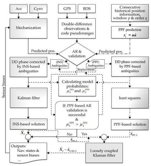However, the methods in [25,26,27] were only proposed to enhance the performance of the GNSS. For GNSS and INS integration, the INS predictions may be affected by gross errors existing in the IMU measurements. Thus, using PPF as an auxiliary model to aid the inertial dynamic model may improve the performance of GNSS/INS integration due to their complementary characteristics. Hence, when abnormal INS predictions are detected, one can use the position predicted by the constructed polynomial fitting model as an alternative. In this paper, we propose a PPF-aided GPS/BDS RTK and INS integration method to estimate the navigation solution in order to achieve continuous and reliable solutions for both ambiguities and positioning performance. We also propose the use of the model probabilities for both the INS and PPF models together with the ambiguity fixing state to detect an epoch with abnormal predictions. The PPF will be triggered once an epoch with abnormal predictions is detected. Furthermore, the full ambiguity resolution (FAR) and PAR strategies are respectively embedded into the proposed method while fixing the float ambiguities.

The typical characteristics of the proposed method when comparing with some existing methods in the domain of GNSS and INS integration are threefold: (i) with the aid of the predicted position from PPF, the proposed method has the ability to resist the abnormal predictions from INS. These abnormal predictions cannot be handled by the commonly used GNSS/INS integrated methods, e.g., [4,11], where no constraints on dynamic model error were introduced. (ii) The adaptive estimation and RAIM methods for GPS/INS integration as presented in [18,19], respectively, could alleviate the impact of abnormal INS predictions. However, these two kinds of methods cannot make full use of the a priori predicted information by down-weighting the variance-covariance matrix of states and deleting the corresponding abnormal state components. The proposed method uses PPF to compensate for the epochs with abnormal INS predictions, which will retain all the useful information from the INS predictions. (iii) Theoretically, the multiple model approaches [20,21,22,23] could achieve consistent results compared with the proposed method since one can incorporate all possible dynamic models, which will characterize the motion behavior of an object into the alternative dynamic models. However, the multiple model methods require nearly linear computation time as a function of the number of models. We should note that only code observations were considered in the existing methods mentioned in this paragraph. The effectiveness of these methods when considering the phase observations still needs further study.

The remainder of this paper is organized as follows: in Section 2, methods for a single-frequency GPS/BDS/INS tightly coupled Kalman filter, the construction of a positional polynomial motion constraint, and the proposed PPF-aided GPS/BDS RTK and INS integration are presented. The experimental results are presented and discussed in Section 3 and Section 4, respectively. Finally, in Section 5, the conclusions are summarized.

2. Methods

2.1. Conventional Single-Frequency GPS/BDS/INS Tightly Coupled Implementation

2.1.1. Inertial Dynamic Model

For the GPS/INS integration problem, the inertial dynamic model of the INS error model could be described as the following psi-angle error equations [4]:

$$\delta \dot{\mathit{r}}=-{\mathit{\omega }}_{\mathrm{en}}\times \delta \mathit{r}+\delta \mathit{v}$$

(1)

$$\delta \dot{\mathit{v}}=-(2{\mathit{\omega }}_{\mathrm{ie}}+{\mathit{\omega }}_{\mathrm{en}})\times \delta \mathit{v}-\delta \mathit{\psi }\times \mathit{f}+\delta \mathit{g}+\mathit{\nabla }$$

(2)

$$\delta \dot{\mathit{\psi }}=-({\mathit{\omega }}_{\mathrm{ie}}+{\mathit{\omega }}_{\mathrm{en}})\times \delta \mathit{\psi }+\mathit{\epsilon }$$

(3)

where $\delta \mathit{r}$, $\delta \mathit{v}$, and $\delta \mathit{\psi }$ are the position, velocity, and orientation error vectors, respectively. The term $\mathit{f}$ denotes the specific force; $\delta \mathit{g}$ is the gravity uncertainty error vector; ${\mathit{\omega }}_{\mathrm{ie}}$ is the rotation rate of Earth with respect to the inertial frame; ${\mathit{\omega }}_{\mathrm{en}}$ is the rotation rate of the navigation frame with respect to Earth; and $\mathit{\nabla }$ and $\mathit{\epsilon }$ are the accelerometer error and gyro error vectors, respectively. All these terms are parameterized in the north-east-down navigation (NED) frame.

The entire error states, which consist of 27 states, can be written as:

$$\{\begin{array}{ll}\mathit{x}& ={\left[{\mathit{x}}_{Nav}^{\mathrm{T}},{\mathit{x}}_{Acc}^{\mathrm{T}},{\mathit{x}}_{Gyro}^{\mathrm{T}},{\mathit{x}}_{Grav}^{\mathrm{T}},{\mathit{x}}_{Ant}^{\mathrm{T}}\right]}^{\mathrm{T}}\\ {\mathit{x}}_{Nav}& ={\left[\delta r_N,\delta r_E,\delta r_D,\delta v_N,\delta v_E,\delta v_D,\delta {\psi }_N,\delta {\psi }_E,\delta {\psi }_D\right]}^{\mathrm{T}}\\ {\mathit{x}}_{Acc}& ={\left[{\mathit{\nabla }}_{bx},{\mathit{\nabla }}_{by},{\mathit{\nabla }}_{bz},{\mathit{\nabla }}_{fx},{\mathit{\nabla }}_{fy},{\mathit{\nabla }}_{fz}\right]}^{\mathrm{T}}\\ {\mathit{x}}_{Gyro}& ={\left[{\epsilon }_{bx},{\epsilon }_{by},{\epsilon }_{bz},{\epsilon }_{fx},{\epsilon }_{fy},{\epsilon }_{fz}\right]}^{\mathrm{T}}\\ {\mathit{x}}_{Grav}& ={\left[\delta g_N,\delta g_E,\delta g_D\right]}^{\mathrm{T}}\\ {\mathit{x}}_{Ant}& ={\left[\delta L_{bx},\delta L_{by},\delta L_{bz}\right]}^{\mathrm{T}}\end{array}$$

(4)

Here, for the convenience of symbolic representation, the vector $\mathit{x}$ is used to indicate the entire error state vector. The vectors ${\mathit{x}}_{Nav}$, ${\mathit{x}}_{Acc}$, ${\mathit{x}}_{Gyro}$, ${\mathit{x}}_{Grav}$, and ${\mathit{x}}_{Ant}$ represent the specific error states corresponding to navigation, accelerometer, gyroscope, gravity, and lever arm, respectively. The subscripts N, E, and D represent the navigation frame, and the subscripts bx, by, and bz represent the body frame pointing in the forward, right, and down directions; ${\mathit{\nabla }}_b$ and ${\mathit{\nabla }}_f$ represent the accelerometer bias and scale factor; ${\epsilon }_b$ and ${\epsilon }_f$ are the gyro bias and scale factor; and $\delta L_b$ represents lever arm errors. In our processing strategy, the inertial sensor bias errors and gravity errors are modeled as a first-order Gauss–Markov (GM) processes, and the lever arm errors are modeled as random constants.

2.1.2. Observation Model

The observation model of the relative positioning describes the relationship between the double-differenced (DD) observations and the unknown parameters. In a general form, the DD code and carrier phase observation model can be written as:

$$\Delta \nabla {\mathit{\rho }}^{*}=\Delta \nabla {\mathit{\rho }}_0^{*}+\Delta \nabla {\mathit{T}}^{*}+\Delta \nabla {\mathit{I}}^{*}+\Delta \nabla {\mathit{M}}^{*}+\Delta \nabla {\mathit{\epsilon }}_{\rho }^{*}$$

(5)

$$\lambda \Delta \nabla {\mathit{\varphi }}^{*}=\Delta \nabla {\mathit{\rho }}_0^{*}+\Delta \nabla {\mathit{T}}^{*}-\Delta \nabla {\mathit{I}}^{*}+\lambda \Delta \nabla {\mathit{N}}^{*}+\Delta \nabla {\mathit{m}}^{*}+\Delta \nabla {\mathit{\epsilon }}_{\varphi }^{*}$$

(6)

where $\Delta \nabla$ denotes the symbol of the DD operator. The superscript “ * ” is the satellite system index, which, in this paper, can be replaced by the capitals “G” and “C” for GPS and BDS, respectively. The terms $\mathit{\rho }$ and $\mathit{\varphi }$ denote the code pseudorange and carrier phase observations, ${\mathit{\rho }}_0$ is the geometric distance between the receiver and satellite, and $\mathit{T}$ and $\mathit{I}$ stand for the tropospheric and ionospheric delay parameters. The terms $\lambda$ and $\mathit{N}$ represent the carrier phase wavelength and integer ambiguity, $\mathit{M}$ and $\mathit{m}$ are the code pseudorange and carrier phase multipath errors, and ${\mathit{\epsilon }}_{\rho }$ and ${\mathit{\epsilon }}_{\varphi }$ are the code and carrier phase noises.

For the RTK positioning of short baseline, the between-satellite and between-receiver DD model is widely used to eliminate the receiver- and satellite-dependent errors. Therefore, residual DD tropospheric delays after corrections with the standard tropospheric model and the ionospheric delays in Equations (5) and (6) can be ignored. Nevertheless, for long distance kinematic positioning, the residual atmospheric uncertainties cannot be neglected, which should be estimated as unknown parameters.

With the dual-constellation configuration, the strength of the integrated observation model is improved. In our GPS/BDS model, system-specific double-differentiation is adopted. Moreover, compared to those with high elevation satellites, observations at lower elevation angles suffer from more larger atmospheric and multipath errors. To account for that problem, the elevation-dependent weighting scheme ${\sigma }^2={\sigma }_0^2+{\sigma }_0^2/{\sin }^2(e)$ [4] is applied for the un-differenced observations with ${\sigma }_0$, the standard deviation at zenith, and $e$, the elevation angle.

2.1.3. Single-Epoch GPS/BDS RTK Ambiguity Resolution with Inertial Aiding and Tightly Coupled Kalman Filter Solution

The whole process of the tightly coupled Kalman filter (TCKF) solution can be divided into two main steps. The first step uses the least squares method to estimate the float ambiguities and then tries to fix the float ambiguities to their integers. The second step executes the Kalman filter to obtain the final solution, i.e., the navigation parameters, INS sensor biases, gravity uncertainty, and lever arm.

For the first step, we first present the linearized DD GPS/BDS observation equation and the virtual observations corresponding to the INS-predicted position, which are as follows:

$$\underset{{\mathit{l}}_k}{\underbrace{{\left[\begin{array}{c}\Delta \nabla \mathit{\varphi }-\Delta \nabla {\mathit{\rho }}_0\\ \Delta \nabla \mathit{\rho }-\Delta \nabla {\mathit{\rho }}_0\end{array}\right]}_k}}=\underset{{\mathit{H}}_k}{\underbrace{{\left[\begin{array}{cc}{\mathit{H}}_{Nav}& \lambda {\mathit{I}}_{n\times n}\\ {\mathit{H}}_{Nav}& {\mathit{0}}_{3\times n}\end{array}\right]}_k}}{\left[\begin{array}{c}{\mathit{x}}_{Nav}\\ {\mathit{x}}_{Amb}\end{array}\right]}_k+{\left[\begin{array}{c}\Delta \nabla {\mathit{\epsilon }}_{\varphi }\\ \Delta \nabla {\mathit{\epsilon }}_{\rho }\end{array}\right]}_k$$

(7)

$${\mathit{0}}_{3\times 1}=\left[\begin{array}{cc}{\mathit{I}}_{3\times 3}& {\mathit{0}}_{3\times n}\end{array}\right]{\left[\begin{array}{c}{\mathit{x}}_{Nav}\\ {\mathit{x}}_{Amb}\end{array}\right]}_k+\Delta \nabla {\mathit{\epsilon }}_{\mathrm{INS}}$$

(8)

where ${\mathit{l}}_k$ and ${\mathit{H}}_k$ are the observation vector and the coefficient matrix, which are determined by Equation (7). Here, the terms $\Delta \nabla \mathit{\varphi }$ and $\Delta \nabla \mathit{\rho }$ are the carrier phase and code observations corrected with the predicted atmospheric delays; $\Delta \nabla {\mathit{\rho }}_0$ is the DD geometric ranges calculated according to the INS-predicted antenna position and satellite positions; ${\mathit{H}}_{Nav}$ is the receiver-satellite geometry matrix; ${\mathit{x}}_{Amb}$ indicates the DD carrier phase ambiguity error vector; $\Delta \nabla {\mathit{\epsilon }}_{\mathrm{INS}}$ denotes the noise vector of the virtual observations; and the subscripts n and k are the number of DD ambiguities and epoch index, respectively.

The combination of the DD observation equation with the virtual observations yields the following combined observation equation for float ambiguity resolution:

$${\left[\begin{array}{c}\Delta \nabla \widehat{\mathit{\varphi }}-\Delta \nabla {\mathit{\rho }}_0\\ \Delta \nabla \widehat{\mathit{\rho }}-\Delta \nabla {\mathit{\rho }}_0\\ {\mathit{0}}_{3\times 1}\end{array}\right]}_k={\left[\begin{array}{cc}{\mathit{H}}_{Nav}& \lambda {\mathit{I}}_{n\times n}\\ {\mathit{H}}_{Nav}& {\mathit{0}}_{3\times n}\\ {\mathit{I}}_{3\times 3}& {\mathit{0}}_{3\times n}\end{array}\right]}_k{\left[\begin{array}{c}{\mathit{x}}_{Nav}\\ {\mathit{x}}_{Amb}\end{array}\right]}_k+{\left[\begin{array}{c}\Delta \nabla {\mathit{\epsilon }}_{\varphi }\\ \Delta \nabla {\mathit{\epsilon }}_{\rho }\\ \Delta \nabla {\mathit{\epsilon }}_{INS}\end{array}\right]}_k$$

(9)

Using the least-squares algorithm to estimate the parameter vector of Equation (9), the float ambiguities and the corresponding variance-covariance matrix can be obtained. Then, the Least-squares AMBiguity Decorrelation Adjustment (LAMBDA) method is used to obtain the integer-valued ambiguities [28]. When they have passed the ambiguity validation test, the ambiguities can be regarded as correct integers. Then, the ambiguity-fixed carrier phase observations are adopted to adjust the 27 states of Equation (4) using the Kalman filter.

In the second step, the coefficient matrix for the Kalman filter can be written as:

$${\mathit{A}}_k=\left[\begin{array}{ccccc}{\mathit{H}}_{Nav}{\mathit{C}}_n^e& {\mathit{0}}_{m\times 3}& {\mathit{H}}_{Nav}{\mathit{C}}_n^e\left[\left({\mathit{C}}_b^n{\mathit{l}}^b\right)\times \right]& {\mathit{0}}_{m\times 15}& {\mathit{H}}_{Nav}{\mathit{C}}_b^n\end{array}\right]$$

(10)

where ${\mathit{C}}_n^e$ is the rotation matrix from the navigation frame to the earth frame, ${\mathit{C}}_b^n$ is the rotation matrix from the body frame to the navigation frame, ${\mathit{l}}^b$ is the lever arm expressed in the body frame, and the subscript m denotes the number of observations.

For the observation vector ${\mathit{y}}_k$, the DD ambiguity-fixed carrier phase and code observations are used. If the ambiguities cannot be fixed, only the code observations are used to update the state vector. Then, the error state vector ${\widehat{\mathit{x}}}_k$ is estimated by the following Kalman filter formulas:

$${\widehat{\mathit{x}}}_k={\mathit{x}}_k^{-}+{\mathit{K}}_k({\mathit{y}}_k-{\mathit{A}}_k{\mathit{x}}_k^{-})$$

(11)

$${\mathit{Q}}_{{\widehat{\mathit{x}}}_k}=({\mathit{I}}_{27\times 27}-{\mathit{K}}_k{\mathit{A}}_k){\mathit{Q}}_{{\overline{\mathit{x}}}_k}$$

(12)

$${\mathit{K}}_k={\mathit{Q}}_{{\overline{\mathit{x}}}_k}{\mathit{A}}_k^{\mathrm{T}}{({\mathit{A}}_k{\mathit{Q}}_{{\overline{\mathit{x}}}_k}{\mathit{A}}_k^{\mathrm{T}}+{\mathit{Q}}_k)}^{-1}$$

(13)

where ${\mathit{K}}_k$ is the so-called gain matrix, ${\mathit{Q}}_k$ is the DD variance-covariance matrix of the observations, and ${\mathit{x}}_k^{-}$ is the predicted state vector. Since we use the error vector to indicate the state, ${\mathit{x}}_k^{-}$ is indeed a 27 × 1 vector with all its elements equal to zero. The term ${\mathit{Q}}_{{\overline{\mathit{x}}}_k}$ denotes the a priori variance-covariance matrix associated with ${\mathit{x}}_k^{-}$. The minus symbol ($-$) as an exponent of a variable represents a “predicted” quantity; the symbol ($^$) above a variable represents an “estimated” quantity.

Then, the 27 × 1 state vector ${\widehat{\mathit{X}}}_k$ can be obtained by subtracting the estimated error states ${\widehat{\mathit{x}}}_k$ from the INS-predicted states ${\mathit{X}}_k^{-}$, that is:

$${\widehat{\mathit{X}}}_k={\mathit{X}}_k^{-}-{\widehat{\mathit{x}}}_k$$

(14)

Finally, the estimated sensor biases are fed back to compensate the raw INS measurements, and the gravity uncertainty is also fed back into the INS mechanization. Then, the navigation solution is updated based on the estimated navigation states of the previous epoch.

2.2. Construction of Positional Polynomial Motion Constraint

An INS can be used to predict the position, velocity, and attitude of the object on which an inertial measurement unit (IMU) is mounted by using the outputs of an accelerometer and gyroscope measurements. However, when the IMU outputs are contaminated by gross errors, the INS-predicted position will deviate from a reasonable one. This will undoubtedly bias the upcoming ambiguity resolution using Equation (7). Therefore, if another reliable predicted position can be provided, this may guarantee the acquisition of a continuous fixed solution so as to improve the reliability and effectiveness of the integrated system.

At epoch k, the position of the rover antenna is approximated as a polynomial with a q-order fitting coefficient [25,26]. Taking all the p positions within the time window, the PPF model reads as:

$$\begin{array}{c}{\mathit{r}}_{k-p}={\mathit{a}}_0\hfill \\ {\mathit{r}}_{k-p+1}={\mathit{a}}_0+{\mathit{a}}_1\delta t+{\mathit{a}}_2\delta t^2+\cdots +{\mathit{a}}_q\delta t^q\hfill \\ ⋮\hfill \\ {\mathit{r}}_{k-1}={\mathit{a}}_0+{\mathit{a}}_1[(p-1)\delta t]+{\mathit{a}}_2{[(p-1)\delta t]}^2+\cdots +{\mathit{a}}_q{[(p-1)\delta t]}^q,\hfill \end{array}$$

(15)

where $\delta t$ denotes the epoch difference between successive two epochs; ${\mathit{a}}_i(i=0\cdots q)$ denotes a 3 × 1 coefficient vector. Here, p is a predefined time window.

The matrix form of Equation (15) is:

$${\mathit{r}}_{(k-p:k-1)}=\mathit{M}\mathit{a}+\varsigma$$

(16)

where $\mathit{M}=\left[\begin{array}{cccc}1& 0& \cdots & 0\\ 1& \delta t& \cdots & \delta t^q\\ ⋮& ⋮& & ⋮\\ 1& [(p-1)\delta t]& \cdots & {[(p-1)\delta t]}^q\end{array}\right]\otimes {\mathit{I}}_{3\times 3}$; ${\mathit{r}}_{(k-p:k-1)}={\left[\begin{array}{cccc}{\mathit{r}}_{k-p}^{\mathrm{T}}& {\mathit{r}}_{k-p+1}^{\mathrm{T}}& \cdots & {\mathit{r}}_{k-1}^{\mathrm{T}}\end{array}\right]}^{\mathrm{T}}$ and $\mathit{a}={\left[\begin{array}{cccc}{\mathit{a}}_0^T& {\mathit{a}}_1^T& \cdots & {\mathit{a}}_q^T\end{array}\right]}^T$; $\varsigma$ is the corresponding residual error vector.

Accordingly, the coefficients $\mathit{a}$ in Equation (16) can be estimated with the least squares method, i.e.:

$$\widehat{\mathit{a}}={({\mathit{M}}^{\mathrm{T}}{\mathit{Q}}_{{\widehat{\mathit{r}}}_{(k-p:k-1)}}^{-1}\mathit{M})}^{-1}{\mathit{M}}^{\mathrm{T}}{\mathit{Q}}_{{\widehat{\mathit{r}}}_{(k-p:k-1)}}^{-1}{\mathit{r}}_{(k-p:k-1)}$$

(17)

where ${\mathit{Q}}_{{\widehat{\mathit{r}}}_{(k-p:k-1)}}$ is constructed by the position variance-covariance matrix from epoch $k-p$ to $k-1$.

Hence, the position predicted by PPF and its associated variance-covariance matrix at epoch k can then be obtained by the following equations:

$${\mathit{r}}_k^{-}=\mathit{u}\widehat{\mathit{a}}$$

(18)

$${\mathit{Q}}_{{\mathit{r}}_k^{-}}=\mathit{S}{({\mathit{M}}^{\mathrm{T}}{\mathit{Q}}_{{\widehat{\mathit{r}}}_{(k-p:k-1)}}^{-1}\mathit{M})}^{-1}{S}^{\mathrm{T}}$$

(19)

Note from Equation (19) that, when the time window and model order of PPF are set in advance, the precision of the predicted position is mainly related to the variance-covariance matrix ${\mathit{Q}}_{{\widehat{\mathit{r}}}_{(k-p:k-1)}}$. If the positions in the time window are all estimated based on ambiguity-fixed carrier phase observations, centimeter-precision position estimates will be achieved. Then, a stable and even centimeter precision of ${\mathit{r}}_k^{-}$ will maintained.

2.3. Proposed PPF-Aided GPS/BDS RTK and INS Method

With the construction of the PPF model, the position predicted by PPF can be employed to estimate the float ambiguities, which are then fixed to their integers. Therefore, the fixed solution could be obtained with the ambiguity-fixed carrier phase observations. Obviously, the above process is similar to the conventional GNSS-only estimation but uses the PPF-predicted position instead. In the following, for simplicity, we call this the PPF-based solution (i.e., with the 3 × 1 position vector and its variance-covariance matrix), while the tightly coupled GPS/BDS RTK and INS integration as described in Section 2.1.3 is named as the INS-based solution (i.e., with the 27 × 1 state vector and its variance-covariance matrix).

Because of the existence of outliers in IMU measurements, using these measurements to predict the current states will degrade the accuracy of float ambiguity solution; this may subsequently affect the ambiguity fixing and therefore degrade the Kalman filter solution. At this point, the PPF-based solution is used to try to provide extra position information on the current epoch. The following should be noted while combining the PPF-based solution with the INS-based solution: (i) in what conditions the constructed PPF method will be triggered to aid the ambiguity fixing failed by an INS-aided system; (ii) when there are outliers in IMU measurements, the float ambiguities estimated based on INS-predicted positions may not be fixed or may be wrongly fixed to their integers, so no ambiguity-fixed carrier phase can be used for the second step of INS-based solutions; (iii) even with the fixed ambiguities provided by the PPF model, outliers in IMU measurements will bias the INS-based solution in the sense that the INS-predicted states ${\mathit{X}}_k^{-}$ will, to some extent, deviate.

Hence, in response to the former three problems, three strategies are proposed: (i) the model probabilities corresponding to the PPF model and inertial dynamic model are calculated, which are, in this paper, used as one of the indicators to trigger or not trigger the PPF method; (ii) the fixed ambiguities based on the PPF-predicted position can be directly used to replace the float/wrongly fixed ambiguities estimated based on the INS-predicted position; (iii) an additional Kalman filter taking the PPF-based solution as virtual observations is needed, with the aim of updating the INS-based solution. As a result, in the following subsubsections, the proposed PPF-aided GPS/BDS RTK and INS integration is presented in three parts, namely, the calculation of the model probability, the substitution of float/wrongly fixed ambiguities, and updating the INS-based solution.

2.3.1. Model Probability Calculation

Using Bayes’ rule [29], the a posteriori probability of model j when the observation is up to k is given by:

$$\begin{array}{cc}\hfill P\left\{M_j\right|{\mathit{L}}^k\}& =P\left\{M_j\right|{\mathit{l}}_k,{\mathit{L}}^{k-1}\}\hfill \\ & =\frac{p\left\{{\mathit{l}}_k\right|M_j,{\mathit{L}}^{k-1}\left\}P\right\{M_j\left|{\mathit{L}}^{k-1}\right\}}{p\left\{{\mathit{l}}_k\right|{\mathit{L}}^{k-1}\}}\hfill \\ & =\frac{p\left\{l_k\right|M_j,{\mathit{L}}^{k-1}\left\}P\right\{M_j\left|{\mathit{L}}^{k-1}\right\}}{{\displaystyle \sum _{i=1}^{2}p\left\{l_k\right|M_i,{\mathit{L}}^{k-1}\left\}P\right\{M_i\left|{\mathit{L}}^{k-1}\right\}}}(j=1,2),\hfill \end{array}$$

(20)

where the symbol $P\{\cdot \}$ denotes the probability; the symbol $p\{\cdot \}$ denotes the probability density function; the symbol $M_j$ indicates a specific model, which in this paper can be the PPF model ($M_1$) and inertial dynamic model ($M_2$); and the epoch indexes $k$ and $k-1$ in the upper right corner of $\mathit{L}$ indicate the observation set up to $k$ and $k-1$, respectively. The term ${\mathit{l}}_k$ is the observation vector at epoch $k$. As seen from Equation (20), when there are several conditional random variables, Bayes’ rule can be used to switch only some of them.

In Equation (20), the first term on the right-hand side of the last identity is the likelihood function ${\Lambda }_k^j$ for $M_j$ at epoch $k$, which can be calculated by:

$$\begin{array}{cc}\hfill {\Lambda }_k^j& =p\left\{{\mathit{l}}_k\right|M_j,{\mathit{L}}^{k-1}\}\hfill \\ & =\frac{1}{{(2\pi )}^{m/2}{\left|{\mathit{S}}_k^j\right|}^{1/2}}\exp \left(\frac{-{\mathit{l}}_k^{\mathrm{T}}{\left({\mathit{S}}_k^j\right)}^{-1}{\mathit{l}}_k}{2}\right),\hfill \end{array}$$

(21)

where $\mathit{S}$ denotes the variance-covariance matrix of the innovation vector ${\mathit{l}}_k$ of Equation (7). As seen from Equation (7), we use the error state rather than the full state as the parameter vector; the observation vector ${\mathit{l}}_k$ is essentially equivalent to the innovation vector in this case.

The term $P\{M_j|{\mathit{L}}^{k-1}\}$ is the a priori probability ${\mu }_{k-1}^j$ of model $M_j$. When $k=1$, ${\mu }_0^j=P\{M_j|{\mathit{L}}^0\}$ is the a priori information of that model. Consequently, Equation (20) could also be written as:

$${\mu }_k^{\mathrm{PPF}}=\frac{{\Lambda }_k^{\mathrm{PPF}}{\mu }_{k-1}^{\mathrm{PPF}}}{{\Lambda }_k^{\mathrm{PPF}}{\mu }_{k-1}^{\mathrm{PPF}}+{\Lambda }_k^{\mathrm{INS}}{\mu }_{k-1}^{\mathrm{INS}}}\mathrm{and}{\mu }_k^{\mathrm{INS}}=\frac{{\Lambda }_k^{\mathrm{INS}}{\mu }_{k-1}^{\mathrm{INS}}}{{\Lambda }_k^{\mathrm{PPF}}{\mu }_{k-1}^{\mathrm{PPF}}+{\Lambda }_k^{\mathrm{INS}}{\mu }_{k-1}^{\mathrm{INS}}}$$

(22)

where the original superscripts j = 1, 2 in ${\mu }_k^j$ or ${\mu }_{k-1}^j$ are symbolized by PPF and INS, which are used to represent the model probabilities of the PPF and INS models, respectively.

The calculation of the model probabilities of the PPF and INS models is detailed. After estimating the float ambiguities of the respective model, they try to fix them to their integers using the LAMBDA. Then, the two sets of fixed or unfixed (when not passing the ambiguity validation test) ambiguities are used to correct the carrier phase observations, forming the respective innovation vectors. With the innovation vector and its corresponding innovation variance matrix ${\mathit{H}}_k{\mathit{Q}}_{{\overline{\mathit{x}}}_k}{\mathit{H}}_k^{\mathrm{T}}+{\mathit{Q}}_k$, the respective model probability can be calculated by Equation (22).

The reason why Equation (22) can be regarded as an indicator for judging the validity of an ambiguity set is that the innovation in the likelihood function considers the fixed/unfixed/wrongly fixed ambiguity vector; thus, either the unfixed or wrongly fixed ambiguity will enlarge the element in the innovation vector, reduce the value of the corresponding likelihood function, and furthermore decrease the model probability. It needs to be emphasized that the validity of an ambiguity set, in this paper, denotes whether the ambiguity set determined based on the PPF model is more credible than the ambiguity set determined based on INS, and vice versa. The term “validity” has a different meaning in the ambiguity validation test of LAMBDA [28], which is used to evaluate the most credible integer ambiguity set chosen in a candidate group searched based on a float ambiguity set and its variance-covariance matrix. Furthermore, as can be seen from Equation (22), the model probability is determined by two factors, i.e., the likelihood function and the a priori probability of each model. In other words, the model probability at the current epoch contains not only the current ambiguity fixing information but also the ambiguity fixing information of the previous epoch.

We note that if the predictions by both of the two models can correctly or cannot fix their associated ambiguity sets, the values of the likelihood functions will be in the same order for the two models. Then, the model probability of the respective model is mainly dependent on the a priori model probability. In this paper, the initial model probabilities are set to 0.9 and 0.1 for the inertial dynamic model and PPF model, respectively. If one of the ambiguity sets can be correctly fixed by the corresponding model prediction, the model probability of this model will be significantly larger than the other one. This is why one can use the proposed model probability method to detect an abnormal prediction of the corresponding model.

2.3.2. Substitution of INS-Based Float/Wrongly Fixed Ambiguities

The substitution of the INS-based float/wrongly fixed ambiguities by the fixed ambiguities determined based on PPF prediction is described. We should emphasize that the discussions in the following two subsubsections are all based on the idea that the ambiguity set can be correctly fixed by the PPF-predicted position. Hence, when there are outliers in IMU measurements, the ambiguities will, to a great extent, not be fixed or be wrongly fixed to their actual integers based on the INS-predicted position, resulting in deteriorated navigation performance of the INS-based solution. However, since the PPF-predicted position does not depend on the external measurements, it requires only that the positions within the time window are all available [27]. If the ambiguity set can be correctly fixed based on PPF, one can simply use these fixed ambiguities to replace the unfixed/wrongly fixed ambiguities estimated based on INS. Then, the ambiguity-fixed carrier phase observations can still be provided to the INS-based solution. In this way, the continuous high-precision observations can still be maintained. From this point of view, the fixed ambiguities provided by the PPF-predicted position can be regarded as an alternative when INS-based ambiguity fixing fails.

2.3.3. Updating the INS-Based Solution

Updating the INS-based solution with the fixed PPF-based solution is detailed. As has been stated above, this step will be triggered only when the INS-based ambiguity fixing has failed or been wrong.

Although the high-precision carrier phase observations are aided by PPF, the estimated state parameters in Equation (14) may also be biased considering the deviated INS predictions ${\mathit{X}}_k^{-}$. Therefore, an additional loosely coupled Kalman filter (LCKF) taking the PPF-based solution as a virtual observation vector is conducted to update the INS-based solution. This filter loop is similar to the conventional LCKF where the GNSS-derived position/velocity are used to aid the INS [30]. However, in our loosely coupled configuration, the observation vector of the additional LCKF is the difference between the PPF-based solution and the position components of the INS-based solution. The observation equation of the additional LCKF is expressed as:

$$\underset{z_k}{\underbrace{\left[{\widehat{\mathit{r}}}_{\mathrm{PPF},k}-{\widehat{\mathit{r}}}_{\mathrm{INS},k}\right]}}=\underset{B_k}{\underbrace{\left[\begin{array}{ccc}-{\mathit{I}}_{3\times 3}& {\mathit{0}}_{3\times 21}& -{\mathit{C}}_b^n\end{array}\right]}}{\mathit{x}}_{\mathrm{LCKF},k}+{\mathit{\eta }}_k$$

(23)

where ${\widehat{\mathit{r}}}_{\mathrm{PPF},k}$ and ${\widehat{\mathit{r}}}_{\mathrm{INS},k}$ represent the PPF-based solution and the position components of INS-based solution, respectively. The terms ${\mathit{z}}_k$ and ${\mathit{B}}_k$ denote the observation vector and coefficient matrix, which are determined by the above equation. The term ${\mathit{\eta }}_k$ is the corresponding error vector. The negative sign in ${\mathit{B}}_k$ is due to the error states being defined by the approximated states minus the actual ones. The symbol ${\mathit{x}}_{\mathrm{LGKF},k}$ is the state error vector of the LCKF, which is used to distinguish the TCKF state error vector ${\mathit{x}}_k$ of Equation (11).

The a priori state information for the additional LCKF and the observation variance-covariance matrix are chosen from the a posteriori variance-covariance matrix of the INS-based solution and PPF-based solution, respectively. Finally, the PPF-aided INS-based solution is calculated through ${\widehat{\mathit{X}}}_k-{\widehat{\mathit{x}}}_{\mathrm{LCKF},k}$. An overview of the architecture of the PPF-aided GPS/BDS RTK and INS integration is shown in Figure 1.

As shown in Figure 1, the INS mechanization is processed and the PPF model is constructed based on the consecutive historical position information. The raw GPS/BDS observations are double differenced by the individual GPS and BDS system. Two ambiguity sets are resolved with the inertial aiding and the PPF aiding, respectively. A validation test is then followed to verify the ambiguity sets. If undergoing a normal INS prediction and the ambiguities pass the validation test, the ambiguity-fixed phase observations together with the code observations are processed by the TCKF to obtain the INS-based fixed solution. Meanwhile, a GNSS-only solution using the ambiguity-fixed high-precision phase and code observations is estimated by a least squares method, i.e., a PPF-based solution. In this time, no assistance from the PPF-related information (i.e., the fixed ambiguities and the PPF-based solution) is required. When there are outliers in the IMU measurements, the INS predictions may be biased and the biased predictions will result in a failed AR process (i.e., the AR validation test fails, or the AR validation test passes but the ambiguity set is wrongly fixed). Therefore, two criteria are used to judge whether to trigger the steps related to the PPF-aided INS-based solution. The first criterion guarantees that the PPF-based AR is valid. The second criterion states whether the model probability ${\mu }_k^{\mathrm{PPF}}$ calculated based on PPF is larger than the INS counterpart ${\mu }_k^{\mathrm{INS}}$. The criterion of the model probability ${\mu }_k^{\mathrm{PPF}}>{\mu }_k^{\mathrm{INS}}$ used here guarantees that the PPF-based AR is statistically significant compared to the INS-based AR. Hence, updating the INS-based solution with the LCKF will improve the INS-based solution. We should note that there is also a situation in which no gross errors exist in the IMU measurements and the ambiguity fixing states of the INS and PPF model are both failed. In this situation, the PPF-aided INS-based solution will not be triggered. This can be easily derived from the two criteria. The failure of the AR processes may be owing to the quality of the observations and/or the constellation of satellites. At this point, only the code observations are used. The proposed method is expected to provide continuous and highly reliable navigation performance.

3. Results

3.1. Field Test Description

A vehicular test was carried out to evaluate the performance of the developed FFP-aided GPS/BDS RTK and INS tightly coupled method in an urban environment (see Figure 2). Seventy minutes of rover station data with 100 Hz INS data and 1 Hz dual-frequency GPS/BDS data were collected by a NovAtel SPAN-CPT system and a high-grade geodetic GNSS dual-frequency receiver on 19 September 2014. Another same receiver mounted on the roof of a tall building was set up as the reference station. The baseline length of the whole experiment was less than 5 km. The test covered the typical area characterized by foliage, a sub-dense urban canyon, a lake, and an open-sky condition. Hence, the satellite positioning performance was limited because of signal blocking and multipath problems. In this test, the single-frequency GPS/BDS (GPS L1 and BDS B1 phase and code observations) and INS data were processed to validate the proposed method using a single-epoch mode, while the dual-frequency ambiguity-fixed GPS/BDS RTK and INS solution was processed for reference. For evaluating the ambiguity, one can compare the position components of the proposed method with the counterparts of the reference trajectory through a predefined threshold to judge whether the corresponding ambiguities are correct or incorrect fixing. The threshold used in this paper was 0.05 m for three position components.

From Figure 2b, it can be seen that the number of visible satellites of BDS was marginally larger than that of the GPS counterparts during the whole test. From the perspective of position dilution of precision (PDOP) values, however, the PDOPs of BDS are larger than those of the GPS ones, which is due to the current deficiency of the BDS geometry configuration. By combining GPS with BDS, the number of visible satellites is doubled compared with in the GNSS-only system. The PDOPs are significantly improved for the combined GPS and BDS constellation. Figure 2c,d show the velocities in the navigation frame and the vehicle attitudes. It can be seen that the vehicle was moving in a moderate dynamic.

During the test, the standard deviation ${\sigma }_0$ at zenith was empirically set to 3 mm and 0.3 m for the phase and code observations, respectively, and the cutoff elevation was set to 15°. The specifications of the inertial sensor are listed in

Table 1. Specifications of inertial measurement unit (IMU) sensor.

Parameter	Gyroscope	Accelerometer
Bias offset	±20°/h	±50 mg
Bias repeatability	±3°/h	±75 mg
In run stability	1°/h ($1\sigma$)	±0.25 mg ($1\sigma$)
Scale factor stability	1500 ppm	4000 ppm
Angular random walk	0.0667°/$\sqrt{\mathrm{h}}$	55 mg/$\sqrt{\mathrm{Hz}}$

.

3.2. Positional Polynomial Fitting Performance by Simulated Vehicle Trajectories

In order to aid the ambiguity fixing so as to obtain continuous and highly reliable navigation solutions, the necessity of subdecimeter-precision-predicted positions for reliable ambiguity resolution should be confirmed by positional polynomial fitting. In this subsection, both the fitting errors and prediction errors of PPF are presented. For the fitting errors, it is calculated by the mean value of the differences between the fitted position coordinates $\mathit{M}\widehat{a}$ of Equation (16) and the corresponding truth position coordinates within the time window. The prediction errors indicate the difference between the predicted position ${\mathit{r}}_k^{-}$ of Equation (18) and the truth position of epoch k.

How to select the time window p and model order q was studied in [25,26]. It was pointed out that the motion of a vehicle often obeys a low-order polynomial over a short period [27]. Therefore, in this subsection, we chose two sets of polynomial fitting model characterized by p = 4, q = 2 and p = 5, q = 3 to build the kinematic model of PPF, respectively. A straight line vehicle trajectory with variable accelerated motion similar to [27] and a combined straight and curved vehicle trajectory with accelerated and decelerated motion were simulated. All the position coordinates were expressed in the earth frame and then transformed to the navigation frame to show the vehicle trajectories in Figure 3.

As seen from Figure 3, the vehicle is simulated to move with a moderate velocity in these two cases, to try to match the actual motion in an urban environment. The description of the straight line vehicle trajectory with variable accelerated motion is separated into the following nine scenarios:

S1 (1–100 s): stationary;

S2 (101–110 s): accelerated motion with 0.8 m/s² in z-axis components;

S3 (110–210 s): uniform motion with velocity 8 m/s in z-axis components;

S4 (211–220 s): variable accelerated motion with 0.1 m/s³ in z-axis components;

S5 (221–320 s): uniform motion with velocity 13.5 m/s in z-axis components;

S6 (321–330 s): variable accelerated motion with −0.1 m/s³ in z-axis components;

S7 (331–430 s): uniform motion with velocity 13.5 m/s in z-axis components;

S8 (431–440 s): decelerated motion with velocity −0.8 m/s² in z-axis components;

S9 (441–540 s): stationary.

The description of the combined straight and curved vehicle trajectory with accelerated and decelerated motion is separated into the following nine scenarios:

S1 (1–50 s): stationary;

S2 (51–60 s): accelerated motion with 1 m/s² in z-axis components;

S3 (61–110 s): uniform motion with the velocity at the end of S2;

S4 (111–155 s): left turning motion with slightly changed velocities;

S5 (156–205 s): uniform motion with the velocity at the end of S4;

S6 (206–255 s): circle motion with slightly changed velocities;

S7 (256–405 s): uniform motion with velocity at the end of S6;

S8 (406–410s): decelerated motion with velocity −2 m/s² in z-axis components;

S9 (411–460s): stationary.

The fitting and prediction errors of the two vehicle trajectory using PPF with different model orders and time windows are shown in Figure 4 and Figure 5. The position coordinates within the time window are simulated as a normal distribution with a zero mean and a standard deviation of 0.01 m. The sampling interval of the position was set to 1 s.

3.3. Full Ambiguity Resolution and Positioning Performance

In terms of the different satellite system combinations, the INS-based solutions, in this paper, can be classified into the following three schemes: GPS/INS, BDS/INS, and GPS/BDS/INS. Furthermore, if the PPF method is considered, the PPF-aided INS-based solutions can also be classified as GPS/INS-PPF, BDS/INS-PPF, and GPS/BDS/INS-PPF schemes. In this subsection, the RTK/INS solutions of different system combinations with or without PPF aiding, together with the GNSS-only solutions with or without PPF aiding, are estimated using a single-frequency single-epoch FAR strategy. The GNSS-only solutions with PPF aiding could be regarded as the application of the method of [25] in integrated navigation with phase observations. Other methods that could be used to handle the abnormal predictions from the dynamic system—such as the adaptive estimation method [18], RAIM method [19], and multiple model method [23]—are not considered here for numerical analyses due to their shortcomings as summarized in Section 1.

Table 2. Single-frequency single-epoch ambiguity fixing states by different schemes using full ambiguity resolution (FAR).

Scheme	Number of Epochs with Fixed Ambiguities (Fixing Rate (%))	Number of Epochs with Incorrectly Fixed Ambiguities (Incorrect Fixing Rate (%]))
GPS	755 (18.38)	41 (5.43)
BDS	769 (18.72)	42 (5.46)
GPS/BDS	3343 (81.38)	0 (0)
GPS-PPF	984 (23.08)	32 (3.38)
BDS-PPF	818 (19.91)	32 (3.91)
GPS/BDS-PPF	3182 (77.46)	0 (0)
GPS/INS	3532 (85.98)	89 (2.52)
BDS/INS	3599 (87.61)	14 (0.39)
GPS/BDS/INS	3529 (85.91)	0 (0)
GPS/INS-PPF	3537 (86.10)	81 (2.29)
BDS/INS-PPF	3634 (88.46)	11 (0.30)
GPS/BDS/INS-PPF	3580 (87.15)	0 (0)

lists the number of epochs with fully and incorrectly fixed ambiguities and their fixing and incorrect fixing rates.

In Table 2, the fixing rate ($P_{\mathrm{FR}}$) and incorrect fixing rate ($P_{\mathrm{IFR}}$) are defined by:

$$P_{\mathrm{FR}}=\frac{\text{number of epochs with fixed ambiguities}}{\text{total number of epochs}}\times 100\%$$

(24)

$$P_{\mathrm{IFR}}=\frac{\text{number of epochs with incorrectly fixed ambiguities}}{\text{total number of epochs with fixed ambiguities}}\times 100\%$$

(25)

It should be noted that the number of epochs with fixed ambiguities mentioned here indicates the number of epochs for which the full set of ambiguities is fixed to their integers. This is used to distinguish the number of epochs with partially fixed ambiguities mentioned in the next subsection, which indicates the number of epochs for which only a subset of ambiguities is fixed to integers.

To further investigate the effectiveness of the schemes with the PPF-aided method, an error with a size of 0.05 g was added to the output of the accelerometer z-axis at GPS time 460,270 s. The position errors and ambiguity fixing states around this epoch are shown in Figure 6. Figure 7 shows the model probabilities calculated by the three PPF-based schemes.

Furthermore, another experiment was performed where errors with a size of 0.05 g were added to each output of the accelerometer axes at GPS time 460,270 s. The position errors, ambiguity fixing states, and model probabilities are presented in Figure 8 and Figure 9.

3.4. Partial Ambiguity Resolution and Positioning Performance

To further improve the ambiguity fixing rate so as to achieve continuous high-precision positioning results, the partial ambiguity resolution (PAR) strategy is added to the ambiguity fixing processes of INS-based AR and PPF-based AR. The PAR used in this paper is conducted in an iterative way, which uses an already-fixed subset of ambiguities as precise ranges to resolve the remaining unfixed ambiguities until all the ambiguities are fixed or there are no more ambiguities that can be fixed.

The vital step for PAR is the selection of an ambiguity subset that can be reliably fixed. In this paper, we chose the commonly used strategy to determine the subset of ambiguities by successively increased elevations. The PAR is only activated if the full ambiguity resolution fails. If FAR fails, the cutoff elevation is then increased by 5°. Therefore, the subset of ambiguities is chosen based on the new cutoff elevation threshold. The LAMBDA method is used to try to fix the subset ambiguities to their integers. If the fixed ambiguity subset does not pass the ratio test and the success rate is lower than the predefined value, this procedure is repeated until a selected ambiguity subset that can be successfully fixed or is empty is obtained. If the fixed ambiguity subset passes the ratio test and the success rate fulfills the predefined value, we think that the subset ambiguities are correctly fixed. Then, the ambiguity-fixed carrier phase observations can be used as precise ranges and aid the fixing of the remaining ambiguities. If none of the ambiguities can be fixed, only the code observations are used and the float solution of the state vector is achieved. The ratio test value and the success rate for PAR are set to 3 and 0.99, respectively.

Table 3. Single-frequency single-epoch ambiguity fixing states with different schemes using partial ambiguity resolution (PAR).

Scheme	Number of Epochs with Fixed Ambiguities (Fixing Rate (%))	Number of Epochs with Partially Fixed Ambiguities (Partial Fixing Rate (%))	Number of Epochs with Incorrectly Fixed Ambiguities (Incorrect Fixing Rate (%))
GPS/INS	3779 (91.99)	301 (7.33)	14 (0.34)
		4080 (99.32)
BDS/INS	3848 (93.67)	84 (2.04)	15 (0.36)
		3932 (95.71)
GPS/BDS/INS	3701 (90.09)	406 (9.88)	0 (0)
		4107 (99.97)
GPS/INS-PPF	3792 (92.31)	288 (7.10)	14 (0.34)
		4080 (99.32)
BDS/INS-PPF	3851 (93.74)	80 (1.95)	15 (0.36)
		3931 (95.69)
GPS/BDS/INS-PPF	3717 (90.48)	390 (9.49)	0 (0)
		4107 (99.97)

lists the single-frequency single-epoch ambiguity fixing states of each scheme using PAR. To demonstrate a clear effect of PPF in aiding GNSS/INS solutions by using PAR, in this subsection, only the integrated solutions are considered. In Table 3, an additional column containing the number of epochs with partially fixed ambiguities and the partial fixing rate is presented, compared with Table 2. The partial fixing rate ($P_{\mathrm{PFR}}$) is computed as:

$$P_{\mathrm{PFR}}=\frac{\text{number of epochs with partially fixed ambiguities}}{\text{total number of epochs}}\times 100\%$$

(26)

In order to manifest the advantage of the proposed PPF-aided method, errors with a size of 0.05 g were added to each output of the accelerometer axes at GPS time 460,270 s in the same way as in the second simulation in Section 3.2. The position errors and ambiguity fixing states around GPS time 460,270 s estimated by the schemes using PAR are shown in Figure 10. The corresponding model probabilities calculated by the schemes with the PPF-aided method using PAR are shown in Figure 11.

To give an overall comparison of the number of ambiguities fixed by PAR and FAR, the ratio of the number of ambiguities ($\Delta P_{\mathrm{FR}}$) fixed by PAR with respect to those fixed by FAR is defined as:

$$\Delta P_{\mathrm{FR}}=\frac{\text{number of ambiguities fixed by PAR-number of ambiguities fixed by FAR}}{\text{number of total ambiguities}}\times 100\%$$

(27)

The $\Delta P_{\mathrm{FR}}$ results corresponding to the integrated solutions are shown in Figure 12.

Finally, in Figure 13, Figure 14 and Figure 15, the performance of each PPF-based scheme using PAR is evaluated by analyzing the positioning errors and the number of fixed DD ambiguities.

4. Discussion

4.1. Discussion on the Performance of the Positional Polynomial Fitting Constraint

Generally, the fitting errors shown in the top two subplots of Figure 4 and Figure 5 are at the centimeter level, which verifies that the PPF model can be well established by the respective model order and its associated time window. However, the prediction accuracy plays a key role in aiding the ambiguity resolution.

As can be seen from the bottom two subplots of Figure 4, the prediction errors are at the subdecimeter level, except for some epochs with large dynamic changes. Even though the prediction errors of the second-order PPF model are marginally smaller than those of the third-order PPF model when there is no dynamic change, the prediction errors of the second-order PPF model are larger than those of the third-order PPF model when undergoing dynamic change, especially for the epochs during S4 and S6, where variable accelerated motions are implemented. This can be seen from the bottom-left subplot of Figure 4; the prediction errors during S4 and S6 (labeled by black frames) fluctuate, while this phenomenon cannot be explicitly seen from the bottom-right subplot of Figure 4. This is because a third-order PPF model can better characterize the variable accelerated behavior than a lower order PPF model.

Similar results can also be seen from the bottom two subplots of Figure 5, where the combined straight and curved vehicle trajectory is considered. We should note that the position coordinates are badly predicted by the second-order PPF model when carrying out a circle motion with the speed at nearly 10 m/s. Nevertheless, the third-order PPF model can still specify this complicated movement. Overall, considering the situation of our field test, a third-order PPF model with the time window set to five is employed.

4.2. Discussion on the Full Ambiguity Resolution and Positioning Performance

As can be seen from Table 2, the fixing rates for single-frequency single-epoch GPS and BDS are low, only 18.38% for GPS and 18.72% for BDS. These can also be seen from the number of epochs with fixed ambiguities for GPS and BDS. Moreover, the incorrect fixing rates of GPS and BDS reach 5.43% and 5.46%, respectively. All these results show that it is difficult for a single-frequency GNSS-only method to achieve reliable dynamic positioning results, considering the limited ambiguity resolutions of them. However, with the combined GPS and BDS system, the fixing rate is greatly improved, reaching 81.38%. This can be attributed to the enhanced satellite geometry and the redundancy of observations, which improve the precision of the float ambiguity estimates. The benefit of the GPS/BDS system is even more obvious in terms of the incorrect fixing rate, reaching 0% for the combined system.

If GPS or BDS is aided by INS, the fixing rate can be improved to more than 80%, exceeding the fixing rate of the GPS and BDS combined system in our experiment. The incorrect fixing rates of GPS/INS and BDS/INS are greatly decreased compared with the GNSS-only case. It is thus evident that the INS-predicted position information benefits the AR performance. This is because the additional INS-predicted position information enhances the variance-covariance matrix of the estimated float ambiguities, which defines the ambiguity search space and the quality of the float ambiguity estimates. However, the incorrect fixing rate of GPS/INS is higher than that of BDS/INS. We find from the GPS/INS solution that the epochs with incorrectly fixed ambiguities are concentrated in a successive period of epochs. This may be due to the quality of the observations during those epochs, and some quality control methods should be introduced to delete those deficient observations in future work. Although the fixing rate of GPS/BDS/INS is slightly lower than the fixing rates of GPS/INS and BDS/INS, the incorrect fixing rate of GPS/BDS/INS equals 0%, which mean that the positioning results are more reliable than the counterparts of GPS/INS and BDS/INS.

If PPF is constructed and is regarded as a dynamic model for GNSS, then the a priori information of the position could be provided so as to assist the ambiguity solution. In Table 2, slightly more epochs could be fixed by GPS and BDS-only schemes with PPF aid. Furthermore, the incorrect fixing rates of the two schemes are also improved compared with those of their respective counterparts without PPF aid. However, the combined GPS and BDS solution with PPF aid becomes worse than the GPS/BDS solution in terms of the ambiguity fixing rate. Based on these results, one can conclude that only taking the PPF as a dynamic model cannot stably improve the ambiguity fixing rate. This is because the PPF is vulnerable to the position accuracy within the time window and the motion of the object.

Hence, if the object’s motion is mainly described by INS and the PPF is regarded as a subordinate model, which will only be triggered when INS model cannot work, the results are improved. We find that the fixing rates of PPF-aided GPS/INS, BDS/INS and GPS/BDS/INS are slightly higher than those of their counterparts without PPF aid. Furthermore, the incorrect fixing rates of PPF-aided GPS/INS and BDS/INS are lower than those of their counterparts without PPF aid. The incorrect fixing rate of PPF-aided GPS/BDS/INS still remains zero. The improvements of the schemes with PPF aid reflect that the INS-predicted position, in some epochs, does not contribute to successful ambiguity fixing, while, in these epochs, the PPF-aided method is triggered, providing correctly fixed ambiguities and updating the INS-based solutions. The effectiveness of the schemes with PPF aid may be more significant when a lower-cost IMU is equipped.

As seen from Figure 6, the position errors for the six schemes are all at the centimeter level before GPS time 460,270 s; in other words, with a reliable INS-predicted position, all six schemes could achieve reliable ambiguity-fixed solutions. However, when there are outliers in the IMU measurements, the navigation performances of the three INS-based solutions visibly deteriorated; at the same time, the ambiguity fixing states became unfixed. Furthermore, for the GPS/INS and BDS/INS schemes, it will take a long time to re-fix the unfixed ambiguities than with the GPS/BDS/INS scheme, as shown in the left three subplots of Figure 6.

When it is detected that there are outliers in the IMU measurements, the PPF-predicted position can still provide reliable position information so as to aid and update the unfixed ambiguities as well as the biased INS-based solutions. The right three subplots of Figure 6 show that continuous and reliable positioning results can be achieved by the three schemes with PPF aid. However, there are a few epochs whose ambiguity sets cannot be fully fixed. This may be due to the specific processing scheme and the quality of the observations of those epochs. However, the ambiguity sets can be immediately fixed right after the unfixed epochs. This is because the ambiguities, in this paper, are resolved in an epoch-by-epoch mode, and when there are no abnormal dynamic predictions, the ambiguity fixing state at previous epochs will not affect the AR performance at the current epoch. Furthermore, the positioning results for the epochs after a g error is introduced will be roughly equivalent to the results where no abnormal INS predictions occur at GPS time 460,270 s.

The model probabilities of the PPF and inertial dynamic models calculated by the three PPF-aided RTK/INS integrated schemes are shown in Figure 7. When the outputs of the IMU contain gross errors at GPS time 460,270 s, the model probability of the INS suddenly decreases to 0.008, while the model probability of PPF increases to 0.992. After one to two epochs, however, the model probability corresponding to INS returns to 0.999. This verifies that with the aid of PPF, the impact of outliers in the IMU measurements on subsequent epochs is greatly reduced. Consequently, the PPF-aided system quickly restores to an INS-aided integration system from the perspective of model probability. The proposed model probability method has the ability to sensitively sense the abnormal predictions caused by IMU measurements with gross errors.

When errors with a size of 0.05 g were added to each output of the accelerometer axes at GPS time 460,270 s, similar positioning performance could be seen as shown by Figure 8 compared with the subplots of Figure 6. The relatively larger outliers in the IMU measurements do not impact the overall positioning performance of the PPF-aided RTK/INS integrated schemes but have a slight impact on the AR performance. This can be seen from the right subplots of Figure 8, where more than one unfixed epoch is found in the GPS/INS-PPF and BDS/INS-PPF schemes, compared with the corresponding subplots of Figure 6. In Figure 8, the positioning results for the epochs after re-convergence are also similar to their counterparts in Figure 6. We note that once the results are convergent, the positioning results for converged epochs will be at the centimeter level if no other factors affect successful AR. From Figure 9, it can be seen that the variation of the curve still verifies the effectiveness of the calculated model probabilities. Theoretically, the larger the outliers in the IMU measurements, the more easily the model probability reflects the actual situation.

4.3. Discussion on the Partial Ambiguity Resolution and Positioning Performance

By comparing the second columns of Table 2 and Table 3, it can be seen that the number of epochs with fully fixed ambiguities with each scheme using PAR is larger than those using FAR. The fixing rates of all the schemes are higher than 90% when the PAR technique is adopted. Moreover, with the PAR, there are epochs where the subset of ambiguities is fixed. The second row of each scheme lists the results by numerically adding the fully fixed results to the partially fixed results. We can find that more than 95% of the epochs can achieve fixed solutions by using PAR, especially for the GPS/INS, GPS/BDS/INS, GPS/INS-PPF, and GPS/BDS/INS-PPF schemes; the full and partial fixing rates of them exceed 99%. In terms of the incorrect fixing rate, the GPS/INS and GPS/INS-PPF schemes using PAR have a great improvement compared with their counterparts using FAR. However, the number of epochs with incorrectly fixed ambiguities obtained by BDS/INS-PPF using PAR is slightly more than that obtained by BDS/INS-PPF using FAR. However, considering that relatively many epochs of fixed solutions can be obtained by the BDS/INS-PPF scheme using PAR, the deficiency in the incorrectly fixed rate is moderate. The most reliable and continuous high-precision positioning results can be achieved by the GPS/BDS/INS and GPS/BDS/INS-PPF schemes using PAR. It is noteworthy that the performance of these two schemes, in this test, is equivalent. This could be attributed to three factors, namely, the strengthened satellite geometry of the combined GPS and BDS system, the utilization of the PAR strategy, and, especially, the fact that there were no significant outliers in the IMU measurements during the whole test. Therefore, the constructed PPF model could hardly be triggered.

When errors with a size of 0.05 g were added to each output of the accelerometer axes at GPS time 460,270 s, the three INS-based solutions were biased due to the outliers in IMU measurements, even with the PAR strategy, as shown by the left three subplots of Figure 10. The PAR can help to achieve continuous and reliable positioning results but is not essential for the adaptivity of an integrated system. Although there are some epochs between the last fixed epoch and the first re-fixed epoch where the ambiguity subsets can be fixed, it is not sufficient to converge the divergent positioning results. With the aid of the PPF model, the continuity and reliability of the positioning results are maintained. The centimeter-level positioning errors are shown in the right three subplots of Figure 10. We should note that the ambiguity fixing states have an obvious improvement compared with the right three subplots of Figure 8, where the FAR strategy is adopted. There are fewer epochs with the fixing states equal to zero when combining PAR with PPF-aided RTK/INS integrated schemes. Similar to the schemes using FAR, once the results are convergent after GPS time 460,270 s, the ambiguity-fixed positioning results will hold if no other factors affect successful AR.

As shown in Figure 11, the model probabilities calculated by the PPF-aided RTK/INS integrated schemes also verify the ability of the proposed model probability method to detect the outliers in the IMU measurements. It is interesting that there are two changes in the model probability curve in the first and third subplots of Figure 11, indicating that the PPF method is triggered twice during this time period. The first change takes place when there are outliers in the IMU measurements as has been explained in Section 4.2, while the second change is due to the use of PAR. The reasons for the second change in the model probability curves can be explained by the following aspects. Taking the GPS/BDS/INS-PPF scheme using FAR and the same scheme using PAR as examples, we can find that there is one epoch with its ambiguity set unfixed in the last subplot of Figure 8, while the ambiguity set of that epoch can be partially fixed as shown in the last subplot of Figure 10. This is because the likelihood function calculated based on the ambiguity-unfixed phase observations is numerically smaller than the counterpart calculated based on the partially fixed phase observations. Furthermore, as can be seen from the last subplot of Figure 11, the second changes for the two curves reflect that there are no ambiguities or wrong ambiguities that can be fixed by GPS/BDS/INS (PAR), while the PPF-aided GPS/BDS/INS (PAR) scheme can correctly fix a subset of ambiguities. Therefore, in that epoch, the model probability based on PPF is significantly larger than the one based on INS. This change in the model probability is found to be consistent with the actual experimental situation when checking the test date, which again verifies the sensitivity of the model probability method in detecting situations with abnormal predictions.

In Figure 12, the $\Delta P_{FR}$ results of the six schemes are greater than or equal to zero in the majority of epochs. This means that the PAR strategy does have the ability to fix more ambiguities than FAR, particularly for the GPS/BDS/INS and PPF-aided GPS/BDS/INS schemes. For the dual-constellation and INS configurations, the number of epochs with $\Delta P_{\mathrm{FR}}$ = 100% is significantly larger than the that for the single-constellation and INS configurations, which shows that with an additional satellite system, the PAR strategy is rather beneficial for fixing the whole set of ambiguities. There are two to four epochs with $\Delta P_{\mathrm{FR}}<0$ when using the single-constellation and INS configurations, which indicates that in these epochs, the FAR can fix all the ambiguities while the PAR can only fix a subset of the ambiguities. However, when checking the positioning results from the epochs with $\Delta P_{\mathrm{FR}}<0$, the positioning errors using FAR reach the decimeter level, which reveals that wrongly fixed ambiguities exist in those epochs. The positioning errors using the PAR in those epochs are at the centimeter level with the exception of one epoch with $\Delta P_{\mathrm{FR}}$ = −14.29% at GPS time 460,679 s of the BDS/INS and PPF-aided BDS/INS schemes, whose positioning errors reach the decimeter level. All in all, the schemes using PAR tend to fix more reliable ambiguities than the FAR strategy, which is of great benefit when continuous and reliable high precision positioning solutions are needed. On the other hand, continuous and reliable high precision positioning solutions are also a prerequisite for the reliable prediction of the PPF model. In this aspect, the PAR strategy is more attractive when a PPF model is considered.

The positioning results of the three PPF-aided RTK/INS integrated schemes are shown in Figure 13, Figure 14 and Figure 15. As can be seen from Figure 13 and Figure 14, the positioning errors are generally at the centimeter level except for a few epochs where the errors are larger than 0.1 m. Epochs with larger positioning errors are usually found when fewer ambiguities can be fixed. The most attractive positioning results are achieved with the PPF-aided GPS/BDS/INS scheme using PAR as shown in Figure 15. The positioning errors are all within 0.06 m during the whole test period, and at least six DD ambiguities can be fixed at each epoch. We note that the better performance of the PPF-aided GPS/BDS/INS scheme by using PAR is attributed to three aspects: (i) the PAR strategy used in this paper can help to fix as many ambiguities as it could; (ii) an additional satellite system can strengthen the satellite geometry and improves the redundancy of the observations; and, furthermore, (iii) with the aid of the PPF model, the adaptivity of the integrated system is also guaranteed. Therefore, good AR performance and positioning results could be obtained from the PPF-aided dual-constellation and INS configuration by using PAR.

5. Conclusions

Reliable and continuous ambiguity resolution is a prerequisite for high-precision positioning using carrier phase observations. However, a challenge is efficient ambiguity and positioning resolution in a single-frequency GNSS/INS integrated system with abnormal INS predictions, especially for the use of a low-cost IMU. In this paper, we have proposed a PPF-aided GPS/BDS RTK and INS integration aiming to compensate for the epochs with abnormal INS predictions. The key to using PPF is to use its predicted current position information to fulfill a successful AR process so as to accomplish an independent GNSS-only solution with ambiguity-fixed phase observations (i.e., the PPF-based solution). The main purpose of PPF is to use its fixed ambiguities and the PPF-based solution to replace the unfixed ambiguities and update the biased float solution of GPS/BDS RTK and INS integration. Moreover, a partial ambiguity resolution strategy is adopted to replace the FAR in order to further improve the ambiguity fixing rate and the positioning solutions. The performance of PPF-based GPS/BDS RTK and INS integration has been evaluated in terms of ambiguity fixing states and positioning solutions through a field vehicular test. The following conclusions can be drawn:

(i)

With the aid of PPF, the fixing rates of the GPS/INS, BDS/INS, and GPS/BDS/INS schemes using FAR are all greater than 86%, higher than their counterparts without PPF aid. Furthermore, the incorrect fixing rates of PPF-aided GPS/INS and BDS/INS are lower than the ones without PPF aid. However, the incorrect fixing rate of PPF-aided GPS/BDS/INS remains 0%. All these results indicate that the proposed PPF method indeed benefits the improvements in AR performance.

(ii)

Further improvement of AR and positioning performance could be obtained by resolving a subset of ambiguities instead of the full set. A success rate greater than 90% can be obtained for all single- or dual-constellation and INS integrations with or without PPF aid. In terms of the incorrect fixing rate, it remains at 0% if dual-constellation systems are considered.

(iii)

If abnormal INS-predicted positions occur, the PPF-aided method can provide ambiguity-fixed phase observations and can help to update the float solution of the GNSS/INS integrated system. As a result, a continuous ambiguity-fixed resolution as well as high-precision and reliable positioning results can be maintained.

(iv)

In order to maintain the reliability of PPF prediction, the continuous and precise positions within the time window are needed. Furthermore, a more continuous and precise positioning solution can be provided with the help of PAR than with the FAR strategy. Therefore, the most attractive option is to combine the PAR with the PPF-aided dual-constellation and INS integration.

To further improve the applicability of the PPF method for a GNSS/INS integrated system, the construction of PPF with different model orders for different dynamic motion should be taken into account. Further research could be pursued by recommending some machine learning algorithms to detect the vehicle motion state, and then the corresponding model order of PPF could be selected on this basis. Moreover, the prediction accuracy of PPF is highly related to the sampling interval, high-rate GNSS data, therefore, will further improve the effect of the proposed method.

References

1. Odolinski, R.; Teunissen, P.J.G. Single-frequency, dual-GNSS versus dual-frequency, single-GNSS: A low-cost and high-grade receivers GPS-BDS RTK analysis. J. Geod. 2016, 90, 1255–1278. [Google Scholar] [CrossRef]
2. He, H.; Li, J.; Yang, Y.; Xu, J.; Guo, H.; Wang, A. Performance assessment of single- and dual-frequency BeiDou/GPS single-epoch kinematic positioning. GPS Solut. 2013, 18, 393–403. [Google Scholar] [CrossRef]
3. Paziewski, J.; Sieradzki, R. Integrated GPS + BDS instantaneous medium baseline RTK positioning: Signal analysis, methodology and performance assessment. Adv. Space Res. 2017, 60, 2561–2573. [Google Scholar] [CrossRef]
4. Han, H.; Wang, J.; Wang, J.; Moraleda, A.H. Reliable partial ambiguity resolution for single-frequency GPS/BDS and INS integration. GPS Solut. 2016, 21, 251–264. [Google Scholar] [CrossRef]
5. Chang, G.; Xu, T.; Chen, C.; Ji, B.; Li, S. Switching position and range-domain carrier-smoothing-code filtering for GNSS positioning in harsh environments with intermittent satellite deficiencies. J. Frankl. Inst. Eng. Appl. Math. 2019, 356, 4928–4947. [Google Scholar] [CrossRef]
6. Han, S.; Wang, J. Integrated GPS/INS navigation system with dual-rate Kalman Filter. GPS Solut. 2011, 16, 389–404. [Google Scholar] [CrossRef]
7. Kim, J.; Kim, Y.; Song, J.; Kim, D.; Park, M.; Kee, C. Performance Improvement of Time-Differenced Carrier Phase Measurement-Based Integrated GPS/INS Considering Noise Correlation. Sensors 2019, 19, 3084. [Google Scholar] [CrossRef] [PubMed] [Green Version]
8. Han, H.; Wang, J. Robust GPS/BDS/INS tightly coupled integration with atmospheric constraints for long-range kinematic positioning. GPS Solut. 2017, 21, 1285–1299. [Google Scholar] [CrossRef]
9. Chang, G. Robust Kalman filtering based on Mahalanobis distance as outlier judging criterion. J. Geod. 2014, 88, 391–401. [Google Scholar] [CrossRef]
10. Li, Z.; Chang, G.; Gao, J.; Wang, J.; Hernandez, A. GPS/UWB/MEMS-IMU tightly coupled navigation with improved robust Kalman filter. Adv. Space Res. 2016, 58, 2424–2434. [Google Scholar] [CrossRef]
11. Li, T.; Zhang, H.; Gao, Z.; Chen, Q.; Niu, X. High-Accuracy Positioning in Urban Environments Using Single-Frequency Multi-GNSS RTK/MEMS-IMU Integration. Remote Sens. 2018, 10, 205. [Google Scholar] [CrossRef] [Green Version]
12. Li, B.; Shen, Y.; Feng, Y.; Gao, W.; Yang, L. GNSS ambiguity resolution with controllable failure rate for long baseline network RTK. J. Geod. 2013, 88, 99–112. [Google Scholar] [CrossRef]
13. Teunissen, P.J.G. Integer estimation in the presence of biases. J. Geod. 2001, 75, 399–407. [Google Scholar] [CrossRef] [Green Version]
14. Henkel, P.; Günther, C. Partial integer decorrelation: Optimum trade-off between variance reduction and bias amplification. J. Geod. 2009, 84, 51–63. [Google Scholar] [CrossRef]
15. Parkins, A. Increasing GNSS RTK availability with a new single-epoch batch partial ambiguity resolution algorithm. GPS Solut. 2010, 15, 391–402. [Google Scholar] [CrossRef]
16. Hewitson, S.; Wang, J. GPS/GLONASS/Galileo receiver autonomous integrity monitoring RAIM performance analysis. GPS Solut. 2006, 103, 155–170. [Google Scholar] [CrossRef]
17. Chang, G. Kalman filter with both adaptivity and robustness. J. Process Control 2014, 24, 81–87. [Google Scholar] [CrossRef]
18. Yang, C.; Shi, W.; Chen, W. Robust M-M unscented Kalman filtering for GPS/IMU navigation. J. Geod. 2019, 93, 1093–1104. [Google Scholar] [CrossRef]
19. Hewitson, S.; Wang, J. Extended Receiver Autonomous Integrity Monitoring (eRAIM) for GNSS/INS Integration. J. Surv. Eng. 2010, 136, 13–22. [Google Scholar] [CrossRef] [Green Version]
20. Blom, H.; Bar-Shalom, Y. The interacting multiple model algorithm for systems with Markovian switching coefficients. IEEE Trans. Autom. Control. 1988, 33, 780–783. [Google Scholar] [CrossRef]
21. Tseng, C.-H.; Chang, C.-W.; Jwo, D.-J. Fuzzy Adaptive Interacting Multiple Model Nonlinear Filter for Integrated Navigation Sensor Fusion. Sensors 2011, 11, 2090–2111. [Google Scholar] [CrossRef] [PubMed] [Green Version]
22. Cho, T.; Lee, C.; Choi, S. Multi-Sensor Fusion with Interacting Multiple Model Filter for Improved Aircraft Position Accuracy. Sensors 2013, 13, 4122–4137. [Google Scholar] [CrossRef] [PubMed]
23. Han, H.; Wang, J.; Du, M. GPS/BDS/INS tightly coupled integration accuracy improvement using an improved adaptive interacting multiple model with classified measurement update. Chin. J. Aeronaut. 2018, 31, 556–566. [Google Scholar] [CrossRef]
24. Moore, M.; Wang, J. An Extended Dynamic Model for Kinematic Positioning. J. Navig. 2003, 56, 79–88. [Google Scholar] [CrossRef] [Green Version]
25. Zhou, Z.; Shen, Y.; Li, B. A windowing-recursive approach for GPS real-time kinematic positioning. GPS Solut. 2010, 14, 365–373. [Google Scholar] [CrossRef] [Green Version]
26. Zhou, Z.; Li, B. GNSS windowing navigation with adaptively constructed dynamic model. GPS Solut. 2014, 19, 37–48. [Google Scholar] [CrossRef]
27. Li, B.; Liu, T.; Nie, L.; Qin, Y. Single-frequency GNSS cycle slip estimation with positional polynomial constraint. J. Geod. 2019, 93, 1781–1803. [Google Scholar] [CrossRef]
28. Teunissen, P.J.G. Least-squares estimation of the integer GPS ambiguities. Invited lecture for “Theory and Methodology”. In Proceedings of the General Meeting of the International Association of Geodesy, Beijing, China, 8–13 August 1993. [Google Scholar]
29. Bar-Shalom, Y.; Li, X.-R.; Kirubarajan, T. Estimation with Applications to Tracking and Navigation; Wiley: Hoboken, NJ, USA, 2001; p. 48. [Google Scholar]
30. Ding, W. Optimal integration of GPS with inertial sensors: Modelling and implementation. Ph.D. Thesis, University of New South Wales, Sydney, Australia, 2008. [Google Scholar]
Figure 1. Architecture of the positional polynomial fitting (PPF)-aided GPS/BeiDou navigation satellite system (BDS) real-time kinematic (RTK) and inertial navigation system (INS) integration. The solid line links the steps of the INS-based solution, the dash-dotted line links the steps of the PPF-based solution, and the dashed line links the steps of the PPF-aided INS-based solution.
Remotesensing 12 02374 g001
Figure 2. Test description of the vehicle experiment: (a) top-left: test trajectory (red line); (b) top-right: number of visible satellites and position dilution of precision (PDOP) values; (c) bottom-left: velocity components and total velocity of the vehicle; and (d) bottom-right: vehicle attitudes.
Remotesensing 12 02374 g002
Figure 3. Simulated vehicle trajectories: (a) left: straight line trajectory and its velocities; (b) right: combined straight and curved trajectory and its velocities.
Remotesensing 12 02374 g003
Figure 4. The fitting and prediction errors of the straight line vehicle trajectory using PPF where max = maximum, min = minimum, and std = standard deviation. The left two subplots show the results corresponding to p = 4, q = 2, and the right two subplots show the results corresponding to p = 5, q = 3.
Remotesensing 12 02374 g004
Figure 5. The fitting and prediction errors of the combined straight and curved vehicle trajectory using PPF where max = maximum, min = minimum, and std = standard deviation. The left two subplots show the results corresponding to p = 4, q = 2, and the right two subplots show the results corresponding to p = 5, q = 3.
Remotesensing 12 02374 g005
Figure 6. Position errors and ambiguity fixing states with different schemes when adding an error with a size of 0.05 g to the output of the accelerometer z-axis at GPS time 460,270 s. A fixing state equal to one indicates that the full set of ambiguities at that epoch is fixed, and zero indicates unfixed. From the top-left to bottom-right, the subplots correspond to the schemes of GPS/INS, BDS/INS, GPS/BDS/INS, GPS/INS-PPF, BDS/INS-PPF, and GPS/BDS/INS-PPF, respectively.
Remotesensing 12 02374 g006
Figure 7. Model probabilities for different PPF-based schemes when adding an error with a size of 0.05 g to the output of the accelerometer z-axis at GPS time 460,270 s. From top to bottom, the subplots correspond to the schemes of GPS/INS-PPF, BDS/INS-PPF, and GPS/BDS/INS-PPF, respectively.
Remotesensing 12 02374 g007
Figure 8. Position errors and ambiguity fixing states with different schemes when adding errors with a size of 0.05 g to each output of the accelerometer axes at GPS time 460,270 s. A fixing state equal to one indicates that the full set of ambiguities at that epoch is fixed, and zero indicates unfixed. From top-left to bottom-right, the subplots correspond to the schemes of GPS/INS, BDS/INS, GPS/BDS/INS, GPS/INS-PPF, BDS/INS-PPF, and GPS/BDS/INS-PPF, respectively.
Remotesensing 12 02374 g008
Figure 9. Model probabilities for different PPF-based schemes when adding errors with a size of 0.05 g to each output of the accelerometer axes at GPS time 460,270 s. From top to bottom, the subplots correspond to the schemes of GPS/INS-PPF, BDS/INS-PPF and GPS/BDS/INS-PPF, respectively.
Remotesensing 12 02374 g009
Figure 10. Position errors and ambiguity fixing states with different schemes when adding errors with a size of 0.05 g to each output of the accelerometer axes at GPS time 460,270 s. A fixing state equal to one indicates that the full set of ambiguities at that epoch is fixed, two indicates that a subset of ambiguities is fixed (partially fixed), and zero indicates unfixed. From top-left to bottom-right, the subplots correspond to the schemes of GPS/INS (PAR), BDS/INS (PAR), GPS/BDS/INS (PAR), GPS/INS-PPF (PAR), BDS/INS-PPF (PAR), and GPS/BDS/INS-PPF (PAR), respectively.
Remotesensing 12 02374 g010
Figure 11. Model probabilities for different PPF-based schemes when adding errors with a size of 0.05 g to each output of the accelerometer axes at GPS time 460,270 s. From top to bottom, the subplots correspond to the schemes of GPS/INS-PPF (PAR), BDS/INS-PPF (PAR), and GPS/BDS/INS-PPF (PAR), respectively.
Remotesensing 12 02374 g011
Figure 12. Ratio of the number of ambiguities fixed by PAR with respect to those fixed by FAR with each scheme. From top-left to bottom-right, the subplots correspond to the schemes of GPS/INS, BDS/INS, GPS/BDS/INS, GPS/INS-PPF, BDS/INS-PPF, and GPS/BDS/INS-PPF, respectively.
Remotesensing 12 02374 g012
Figure 13. Position errors with the PPF-aided GPS/INS scheme and the number of fixed ambiguities using the PAR strategy.
Remotesensing 12 02374 g013
Figure 14. Position errors with the PPF-aided BDS/INS scheme and the number of fixed ambiguities using the PAR strategy.
Remotesensing 12 02374 g014
Figure 15. Position errors with the PPF-aided GPS/BDS/INS scheme and the number of fixed ambiguities using the PAR strategy.
Remotesensing 12 02374 g015