LiDAR/RISS/GNSS Dynamic Integration for Land Vehicle Robust Positioning in Challenging GNSS Environments

Abstract

The autonomous vehicles (AV) industry has a growing demand for reliable, continuous, and accurate positioning information to ensure safe traffic and for other various applications. Global navigation satellite system (GNSS) receivers have been widely used for this purpose. However, GNSS positioning accuracy deteriorates drastically in challenging environments such as urban environments and downtown cores. Therefore, inertial sensors are widely deployed inside the land vehicle for various purposes, including the integration with GNSS receivers to provide positioning information that can bridge potential GNSS failures. However, in dense urban areas and downtown cores where GNSS receivers may incur prolonged outages, the integrated positioning solution may become prone to severe drift resulting in substantial position errors. Therefore, it is becoming necessary to include other sensors and systems that can be available in future land vehicles to be integrated with both the GNSS receivers and inertial sensors to enhance the positioning performance in such challenging environments. This work aims to design and examine the performance of a multi-sensor system that fuses the GNSS receiver data with not only the three-dimensional reduced inertial sensor system (3D-RISS), but also with the three-dimensional point cloud of onboard light detection and ranging (LiDAR) system. In this paper, a comprehensive LiDAR processing and odometry method is developed to provide a continuous and reliable positioning solution. In addition, a multi-sensor Extended Kalman filtering (EKF)-based fusion is developed to integrate the LiDAR positioning information with both GNSS and 3D-RISS and utilize the LiDAR updates to limit the drift in the positioning solution, even in challenging or ultimately denied GNSS environment. The performance of the proposed positioning solution is examined using several road test trajectories in both Kingston and Toronto downtown areas involving different vehicle dynamics and driving scenarios. The proposed solution provided a performance improvement over the standalone inertial solution by 64%. Over a GNSS outage of 10 min and 2 km distance traveled, our solution achieved position errors less than 2% of the distance travelled.

1. Introduction

Reliable positioning and navigation are vital for self-driving car applications. Using position fixing (PF) techniques such as the Global Navigation Satellite System (GNSS), the vehicle can navigate easily in unknown environments. The GNSS provides an absolute long-term positioning solution when in line of sight with four or more satellites. However, reliable GNSS signals are not guaranteed in all environments due to satellite signal blockage, poor satellite geometry, and multipath in dense urban areas [1]. Therefore, the Inertial Navigation System (INS), which is a dead reckoning (DR) technique is usually integrated with the GNSS receiver to provide a positioning solution in case of GNSS failure. The INS is an autonomous system that requires no external information to calculate the location information, unlike the GNSS [2]. The INS consists of inertial sensors such as accelerometers and gyroscopes, which given an initial position, velocity, and attitude, provides a positioning solution [3,4]. However, the positioning solution from the INS has good short-term accuracy, and this is because it suffers from error in sensor measurements accumulating, which requires external information for resetting those errors [5]. The GNSS and the INS have complementary features that led to the trend of integrating both sensors using different filtering techniques to have a more reliable and accurate solution that mitigates each sensor’s drawbacks [6]. The INS/GNSS integrated navigation system is the most popular form of integration in which the GNSS provides measurement updates to the INS via Kalman Filtering (KF). As the GNSS measurements prevent inertial sensors from drifting by resetting their errors, the INS smooth the GNSS solution and provides a solution in the case of GNSS outage. A low-cost micro-electro-mechanical system (MEMS)—based inertial sensors is used to cut the cost of such a navigation system. During the past decade, the performance of low-cost MEMS-based inertial sensors has improved significantly that it has found many uses mainly in the automobile industry [7].

Moreover, a three-dimensional reduced inertial sensor system (3D-RISS) was developed to be integrated with the GNSS to provide a more reliable navigation solution for the land vehicle. The 3D-RISS minimizes the usage of the accelerometers and gyroscopes, therefore, reducing the accumulated drift errors [8]. The 3D-RISS mechanization method is mainly developed for land vehicle navigation as it also utilizes the wheel odometer of the land vehicle, which measures the forward speed of the vehicle to calculate the pitch and roll angles. However, the integrated solution fails to provide a reliable navigation solution in extended outages due to the absence of a GNSS signal to reset the residual biases that accumulate over time.

AVs are anticipated to navigate not only on controlled highways but also in suburban and dense urban areas. The realization of such a goal is based on the development of robust and reliable, fully autonomous systems that can make decisions based on the perception of its sensors [9]. Therefore, autonomous cars house perception sensors that help in positioning the vehicle in these situations. Generally, the most common sensors used for integrating with the INS are cameras, Light Detection and Ranging (LiDAR), and Radio Detection and Ranging (RADAR). Compared to the camera, the LiDAR has higher resolution and can provide detailed structural information of the surrounding area. Also, laser scanners are not affected by ambient light like cameras and have a higher resolution than RADARs. As LiDAR sensors are becoming cheaper and smaller in size, they are becoming more suitable for autonomous vehicle applications. Therefore, the work in this paper utilizes mechanical rotating 3D-LiDAR that provides a 360° panoramic view of the surrounding environment.

As the GNSS becomes unreliable in downtown cores, studies emerged that favored DR solutions such as simultaneous localization and mapping (SLAM) and odometry methods. Those techniques enabled the calculation of the position and orientation of the vehicle based on the data obtained from the onboard sensors. The LiDAR Odometry (LO) is based on the laser reflected from the surrounding objects to estimate the position and orientation given a starting point. A method involving using LO was introduced in [10] to estimate the movement between frames and matches the estimated solution to a road map using particle filtering. Another author in [11] suggested that when the LiDAR scanning rate is higher than the extrinsic motion, the standard Iterative Closest Point (ICP) is used to compute a moving object velocity to address the motion distortion introduced in a single-axis 3D-LiDAR. However, the traditional ICP is computationally expensive, according to the authors in [12]. Using a LiDAR, IMU, and a wheel odometer, the authors in [13], suggested an integration scheme for pose estimation. They used a point-to-plane ICP approach for the registration of the LiDAR point clouds and EKF for multi-sensor fusion and also a point cloud data map. However, their experiments were done in a controlled and previously mapped environment with nearly static scenes. The authors in this work used a point-to-plane approach, which is much faster in terms of computational complexity. However, using a full IMU mechanization along with the proposed ICP increases the overall computational complexity of the system. Another approach is the pose estimation using LO extracted using the ICP and pseudo cellular ranges fused using EKF to estimate the heading of the vehicle accurately in [14]. A GNSS/INS/LiDAR-SLAM integrated navigation system was proposed in [15], where the GNSS/INS result and the relative pose from a 3D probability map were matched with the graph optimizing. However, in [15], the LiDAR’s point cloud was not preprocessed, and thus many errors would increase in such a method.

In this paper, a multi-sensor fusion approach is introduced to bridge GNSS outages and provide reliable and continuous positioning and navigation information. The proposed system is based on integrating LiDAR, INS, and GNSS, supported by a method that smartly selects the best combination from these three systems to provide the most reliable positioning information. The specific contributions of this paper are the following:

• Design and implementation of denoising method for the raw LiDAR point cloud to remove any outliers, thus reducing the computational complexity and enhancing the performance.
• Utilization of the Iterative Closest Point (ICP) algorithm to register the LiDAR point clouds and minimize the root-mean-squared error between two consecutive point clouds.
• Realization of an Extended Kalman Filter (EKF) to fuse the positioning information from GNSS, INS, and LiDAR and improve the overall positioning solution.
• Design and implementation of a selection criterion that can automatically select the set of sensors/systems to be included in the fusion filter to mitigate the drift in the positioning solution.
• The performance of the proposed system is assessed based on road test experiments to quantitively assess its merits and limitations when compared to a high-end reference solution.

The paper is structured as follows. In Section 2, the system architecture LiDAR/RISS/GNSS integrated navigation system is explained along with the mathematical model of the reduced inertial system. In Section 3, the experimental setup is presented. Next, in Section 4, the results are discussed. Finally, Section 5 is the conclusion, along with future work prospects.

2. System Architecture and Mathematical Model

In prolonged and frequent GNSS outages, the INS/GNSS integration suffers from biases and drifts that are modulated with time. The drifts in the INS mechanization are caused due to implicit mathematical integrations associated with the algorithm. In a classic INS mechanization, all the six Degree of Freedom (DoF) IMUs are used, integrating the rotation rates of the 3-axis orthogonal gyroscopes to compute the attitude angles. Therefore, the error in the transformation from the body frame to the local frame will linearly increase in time for every given gyroscope error. Also, since the velocities are calculated by integrating the 3-axis accelerometer readings and then rotating by the attitude angles, the linear gyroscope error becomes quadratic. Eventually, to get the 3D-position, the velocity is integrated again, and the quadratic error becomes cubic order [6]. The land vehicle’s motion has three characteristics that are defined in [16], which prove that three orthogonal gyroscopes, along with a forward accelerometer, are sufficient for land vehicle navigation. However, increasing the number of gyroscopes, as mentioned before, proven to increase the inherent errors from the integration process. Therefore, to further simplify the system, a single gyroscope along with two accelerometers and the vehicle wheel odometer is used to decrease the inherent errors in the system.

2.1. Three-Dimensional Reduced Inertial Sensor System (3D-RISS)

The 3D-RISS utilizes only the vertical gyroscope ($w_z$), the forward accelerometer ($f_x$), and the transversal accelerometer ($f_y$) from the IMU unit along with the wheel odometer of the vehicle. The odometer is used to measure the vehicle’s forward velocity ($v_{od}$) to be differentiated into the acceleration of the vehicle between each epoch to get the vehicle’s forward acceleration ($a_{od}$). Figure 1 gives a detailed description of the mechanization process [17].

The 3D-RISS utilizes the denoised sensor measurements from the ($f_x$, $f_y$, $w_z$) and the measured forward velocity from the odometer as the mechanization inputs. Accordingly, the navigation state vector of the 3D-RISS is given by the following Equation (1):

$$x={\left[\begin{array}{ccccccccc}\phi & \lambda & h& v_e& v_n& v_u& r& p& Azi\end{array}\right]}^T$$

(1)

where ($\phi$, $\lambda$, $h$) corresponds to the 3D-position components, namely the latitude, longitude, and the altitude, respectively. The ($v_e$, $v_n$, $v_u$) represents the velocity components in the local level frame (LLF), the East, North, and Upward velocities, respectively. While ($r$, $p$, $Azi$) are the attitude angles, the roll, pitch, and azimuth. The pitch and roll angles are calculated at each epoch k as follows in Equations (2) and (3).

$$p_k=si{n}^{-1}\left(\frac{f_{y_k}-a_{o{d}_k}}{g}\right)$$

(2)

$$r_k=-si{n}^{-1}\left(\frac{f_{x_k}+v_{o{d}_k}\left(w_{z_k}-b_z\right)}{g\cos \left(p_k\right)}\right)$$

(3)

The bias in the gyroscope readings ($b_z$) is taken into consideration. Also, the azimuth angle is calculated as follows in (4), at each epoch k.

$$Az{i}_k=Az{i}_{k-1}+\left(-\left(w_{z_k}-b_z\right)+w_e\sin \left({\phi }_{k-1}\right)+\frac{v_{e_{k-1}}\tan \left({\phi }_{k-1}\right)}{R_N+h_{k-1}}\right)\Delta t$$

(4)

where ($R_N$) is the normal radius of the earth’s ellipsoid, and ($w_e$) is the earth’s rotation component. Then, using the attitude angles the forward speed measured by the odometer is projected on to the East ($v_{e_k}$), North ($v_{n_k}$), and Upward ($v_{u_k}$) velocity components in the local level frame as illustrated in Equation (5):

$$\left[\begin{array}{c}{v}_{e_k}\\ v_{n_k}\\ v_{u_k}\end{array}\right]=\left[\begin{array}{c}{v}_{o{d}_k}\cos \left(Az{i}_k\right)\cos \left(p_k\right)\\ v_{o{d}_k}\cos \left(Az{i}_k\right)\cos \left(p_k\right)\\ v_{o{d}_k}\sin \left(p_k\right)\end{array}\right]$$

(5)

After that, the 3D-position states, latitude ($\phi$), longitude ($\lambda$), and altitude ($h$) in each epoch are derived from integrating the velocities in the LLF and rotating them using the normal ($R_N$) and meridian ($R_M$) radii, as shown in Equation (6):

$$\left[\begin{array}{c}{\phi }_k\\ {\lambda }_k\\ h_k\end{array}\right]=\left[\begin{array}{c}{\phi }_{k-1}+\frac{0.5\left(v_{n_k}+v_{n_{k-1}}\right)}{R_N+h_k}\mathsf{\Delta }t\\ {\lambda }_{k-1}+\frac{0.5\left(v_{e_k}+v_{e_{k-1}}\right)}{\left(R_M+h_k\right)\cos \left({\phi }_{k-1}\right)}\mathsf{\Delta }t\\ h_{k-1}+0.5\left(v_{u_k}+v_{u_{k-1}}\right)\mathsf{\Delta }t\end{array}\right]$$

(6)

Therefore, by reducing the number of the inertial sensors used, the 3D-RISS reduced the complexity of the system. Also, using the odometer and the accelerometers to calculate the pitch and roll angles rather than the gyroscopes eliminates the need for numerical integration. Therefore, no drift or error growth.

2.2. LiDAR Odometry

Scan matching algorithms have been widely popular in recent years as they provide an understanding of the movement of the points between two consecutive scans. The ICP is widely used as it is one of the dominant solutions for aligning three-dimensional models based on the Euclidean distance [18], providing an initial estimate of the relative pose of the vehicle. The accuracy of the registration using ICP is dependent on the number of points and the nature of the scene. Therefore, preprocessing steps are required as navigating in a dynamic environment needs context awareness of objects surrounding the vehicle, which happens in most perception pipelines [19]. Therefore, point cloud segmentation is required before using the ICP to register the point clouds. Figure 2 shows a flowchart of the point cloud preparation.

2.2.1. Ego Points Removal

The 3D-LiDAR used generates an organized point cloud in the form an M-by-N-by-3 array containing the (x, y, z) coordinates of the points in the LiDAR body frame in meters. It also has a 360° horizontal field of view (FOV) and a 30° vertical FOV. It is mounted on the vehicle’s roof, which causes the ego vehicle points to appear in each scan that can affect the ICP algorithm’s accuracy. Therefore, to determine the ego vehicle points in the point cloud, the mounting location of the LiDAR is estimated in the LiDAR body frame considering the vehicle’s dimensions The measurements of the vehicle are defined, as shown in Equation (7), and assuming that the LiDAR is mounted horizontally to the ground plane.

$$Dimensions=\left[X_{min}{X}_{max}{Y}_{min}{Y}_{max}{Z}_{min}{Z}_{max}\right]$$

(7)

where ($X_{min} X_{max}$) corresponds to the width of the vehicle, ($Y_{min} Y_{max}$) corresponds to the length of the vehicle, and ($Z_{min} Z_{max}$) corresponds to the height of the vehicle. With the aid of the vehicle’s entered dimensions, a cube is constructed around the mounting location of the LiDAR. As a result, any points lying inside the constructed cube are considered the ego vehicle points and therefore are eliminated from the scene. Figure 3 shows the ego vehicle points in a point cloud labeled in red.

2.2.2. Segmentation of the Ground Points from the Point Cloud

After removing the ego vehicle points from the point cloud scene, the ground points are removed next from the scene. Also, assuming that the LiDAR is mounted horizontally to the ground plane and that it appears in at least the lowest row of the point cloud. Therefore, an elevation angle ($\alpha$) is set as a threshold and the point of the lowest orientation angle (${\theta }_i$) is labeled as a ground point. Then, the elevation angle is computed between a ground point and its four connected neighbor points. The neighborhood point is labeled as a ground point if the difference is below the specified ($\alpha$). Figure 4 shows the ground points labeled in yellow while the ego vehicle points are labeled in red.

2.2.3. LiDAR Point Cloud Clustering

Point cloud clustering methods have been widely used to group points with similar spectral features into the same homogenous pattern [20]. The 3D-LiDAR used in this work is the Velodyne PUCK LITETM [21], which has 16 channels of individual laser pulse projectors. This LiDAR has a 2° vertical angular resolution, while the horizontal angular resolution ranges from 0.1° to 0.4° depending on the scanning speed. This considerable difference between the vertical and horizontal angular resolutions has an impact on the clustering process. The clusters are created based on the Euclidean distance between the neighboring points A and B. Threshold is set for the maximum distance between two neighboring points. A potential problem would occur when the two laser measurements are within the distance threshold but belong to another object. Therefore, another constraint on the angle between the neighboring points and the LiDAR is employed. A line is created passing through the sensor at O, and point A forms the first side of the angle. The second side of the angle is formed by passing a line through points A and B, as illustrated in Figure 5.

An angle ($\beta$) is formed and defined as the angle between the laser beam from the sensor and the line connecting A and B. If the angle ($\beta$) is greater than the specified angle threshold, then the points are grouped in the same cluster. Figure 6 shows the clustered point cloud with each cluster given a unique color. It was observed that some of the clusters contained one or two points per cluster. Therefore, clusters that contain such little points are discarded from the point cloud scene.

2.2.4. Point Cloud Denoising

The point cloud may contain points that are beyond the scanning range of the LiDAR, or the laser encountered an absorbing material that attenuated the laser pulse. When this phenomenon happens, the LiDAR registers these points in the point cloud as either infinite (Inf) or Not a Number (NaN). However, some points are noisy and irrelevant to the scene, which can cause noisy outputs when using the ICP algorithm. Therefore, the point cloud is denoised to remove the outliers and noise from the scene. The denoising is accomplished based on computing the standard deviation (SD) of the mean of the average distance of the neighbor points, as shown in the following Equation (8):

$$SD=\sqrt{\frac{\sum {\left(D_i-\overline{D}\right)}^2}{N-1}}$$

(8)

where, $D_i$ is the distance measured at a point i, $\overline{D}$ is the mean of the distances of the neighboring point, and $N$ is the number of neighboring points. The term $\left(D_i-\overline{D}\right)$ is the deviation of the distance of point i from the mean. Increasing the number of neighboring points N would increase the number of computations while decreasing it would make the filter more sensitive to noise. As illustrated in Figure 7a shows the raw point cloud while the red circles highlight the most distinctive points that are removed from the scene. Figure 7b illustrates the denoised point cloud.

2.2.5. Point Cloud Downsampling

The 3D-LiDAR generates around 300,000 points per second [21]. Therefore, any scan matching algorithm will require high computation power to process the point cloud [22]. So, the downsampling step is essential to reduce the computational complexity of the scan matching algorithm. Downsampling is achieved by applying a box grid filter on the point cloud. The Grid size is defined based on the manner of not losing any distinctive features in the point cloud scene but reducing the number of points. The downsampling step is considered the most critical parameter of the scan matching algorithm as it controls the speed of the registration. Figure 8a shows the normal point cloud, and Figure 8b shows the downsampled point cloud.

2.2.6. Iterative Closest Point (ICP)

The ICP is the method used in this work to register the point clouds and obtain the translation and rotation between the point clouds. The ICP relies on finding the least square rigid transformation that minimizes the distance between two point cloud sets. Several implementations of the ICP suffer drawbacks as its tendency to diverge if the initial alignment is not proper. This divergence in the ICP is overcome by setting an initial point of (0, 0, 0) in the (x, y, z) coordinates of the LiDAR body frame. A six DoF spatial rigid transformation in three-dimensional Euclidean space is estimated that preserves the Euclidean distance between the point clouds. After the preprocessing done on the point cloud, the ICP algorithm registers the points in the fixed point cloud with the closest point in the moving point cloud to achieve the minimum Root Mean Squared (RMS) error. A point-to-plane approach, which is a variant of the ICP, is applied in this work. This method leverages the advantages of the normal surface information by minimizing the Root-Mean-Squared (RMS) error between a point and its tangent plane to improve robustness and accuracy. The ICP algorithm output consists of a transformation matrix, as shown in Equation (9) and the RMS error in the transformation.

$$Tform=\left[\begin{array}{cccc}cos\left({\theta }_y\right)\ast cos\left({\theta }_z\right)& -sin\left({\theta }_z\right)& sin\left({\theta }_y\right)& 0\\ sin\left({\theta }_z\right)& cos\left({\theta }_x\right)\ast cos\left({\theta }_z\right)& -sin\left({\theta }_x\right)& 0\\ -sin\left({\theta }_y\right)& sin\left({\theta }_x\right)& cos\left({\theta }_x\right)\ast cos\left({\theta }_y\right)& 0\\ \Delta x& \Delta y& \Delta z& 1\end{array}\right]$$

(9)

The $Tform$ is a 4 × 4 matrix that is a combination of the translations and rotations that represent the ways that objects move in the world. The translations are defined as the 4th and last row of the $Tform$ which comprises of ($\Delta x$, $\Delta y$, $\Delta z$). While the angles (${\theta }_x$, ${\theta }_y$, ${\theta }_z$) are the Euler angles that define each rotation in the (x, y, z) directions, respectively.

It is expected that when the vehicle is stationary, pedestrians and cars will be moving in the scene. This phenomenon could lead to incorrect registration of the point clouds, and as a result, significant deviations are imposed on the translations and rotations. However, when the vehicle is stationary, it was observed that the RMS error between the point clouds is minimal in contrast to when the vehicle is mobile. Therefore, when the ICP algorithm starts to work, a few epochs are used at first to calculate an average for the RMS error of the ICP. The RMS error average is used as a threshold to determine if the registration process does not provide reliable measurements. Therefore, an approach to use the vehicle’s odometer with the RMS error to stop the registration of the ICP is introduced due to the correlation of the vehicle’s speed and RMS error of the ICP. A threshold is set at 1 m/s for the vehicle’s velocity. This way, we can ensure that when the car is nearly at rest, this would mean that the RMS error should be less than the average RMS error calculated at first. Therefore, if a spike in the RMS error at low speeds occur, it would not affect the stopping of the ICP registration. Figure 9 shows over 180 s the relation between the RMS error and vehicle’s speed, highlighting the calculated average RMS error of the ICP, which is 0.6 m in this scenario.

The LO output is composed of the displacement and the heading from the initial point (0, 0, 0) to the destination. These movements are the accumulation of the translations in (x, y, z) directions in the LiDAR body frame. These movements are transformed from the body frame to the LLF. The transformation to the LLF requires an initial point with curvilinear coordinates in the LLF (${\phi }_o$, ${\lambda }_o$, $h_o$) to be known along with its heading ($Azi$). After that, the position in the rectangular coordinates (E, N, U) is calculated as follows:

$$\left[\begin{array}{c}\Delta P_{E_k}\\ \Delta P_{N_k}\\ \Delta P_{U{p}_k}\end{array}\right]=\left[\begin{array}{ccc}cos\left(Az{i}_k\right)& -sin\left(Az{i}_k\right)& 0\\ sin\left(Az{i}_k\right)& cos\left(Az{i}_k\right)& 0\\ 0& 0& 1\end{array}\right]\left[\begin{array}{c}\Delta x_k\\ \Delta y_k\\ \Delta z_k\end{array}\right]$$

(10)

where ($\Delta P_{E_k}$, $\Delta P_{N_k}$, $\Delta P_{U{p}_k}$) denotes the change in position in the East, North, and Upward directions at each epoch k in the LLF. The ($\Delta P_{U{p}_k}$) is then accumulated each epoch on the initial altitude to calculate ($h_{LiDA{R}_k}$) as depicted in Equation (11). Then, the ($\Delta P_{N_k}$) and ($\Delta P_{E_k}$) in each epoch are used to obtain the (${\phi }_{LiDA{R}_k}$) and (${\lambda }_{LiDA{R}_k}$) of the geodetic coordinates in Equations (12) and (13), respectively.

$$h_{LiDA{R}_k}=\Delta P_{U{p}_k}+h_{LiDA{R}_{k-1}}$$

(11)

$${\phi }_{LiDA{R}_k}=\frac{\Delta P_{N_k}}{R_M+h_{LiDA{R}_k}}+{\phi }_{LiDA{R}_{k-1}}$$

(12)

$${\lambda }_{LiDA{R}_k}=\frac{\Delta P_{E_k}}{\left(R_N+h_{LiDA{R}_k}\right)\ast cos\left({\phi }_{LiDA{R}_k}\right)})+{\lambda }_{LiDA{R}_{k-1}}$$

(13)

2.3. LiDAR/RISS/GNSS Integration

The LiDAR/RISS/GNSS, an integrated navigation system, is proposed to reset the biases of the inertial sensors in the 3D-RISS solution, as shown in Figure 10. The system utilizes the EKF in a loosely-coupled fashion for the integration. The 3D-RISS is used for prediction, while the switching algorithm toggle the GNSS and LiDAR to provide the measurement updates in the EKF. Nonetheless, if both sensors fail to provide a reliable solution, the 3D-RISS works as a standalone system to provide a navigation solution.

Switching Criterion

In order to maximize the benefits of integrating GNSS, LiDAR, and inertial sensors, we are developing a method to choose the system (GNSS or LiDAR) that is most reliable for integration with RISS. The position measurement update will switch between GNSS and LiDAR. The switching criterion of this Multi-Sensor System (MSS) relies on several factors from the readings of the GNSS receiver, the ICP algorithm, and values from the IMU measurements. This way, a dynamic and robust integrated navigation system in urban environments is introduced. The GNSS receiver provides at each epoch the number of satellites it is observing along with the value of the Geometric Dilution of Precision (GDOP). The GDOP value provides an understanding of the satellite geometry observed by the receiver [1]. Also, the SD of the 3D-position provided by the GNSS indicates the reliability of the GNSS performance. Since an LC integration is utilized, the number of satellites observed plays a massive role in the accuracy of the RISS/GNSS integration. Therefore, the GNSS would fail to provide a reliable solution if the number of satellites observed falls below four. Moreover, if the GDOP value is too high, this would also result in unreliable GNSS measurements. The GDOP is calculated using the parameters of the user’s position and time bias errors, which are the latitude, longitude, altitude, and time to those of the pseudo-range errors from the GNSS:

$$GDOP=\sqrt{q_{xx}+q_{yy}+q_{zz}+q_{tt}}$$

(14)

where the ($q_{xx,}{q}_{yy},q_{zz},q_{tt}$) represent the variance of the estimated user position in each axis and in the user time offset. It is also observed that when the SD of the 3D-position starts to increase in value, the GNSS positioning solution starts to drift from the reference solution. Therefore, depending on the GDOP value, and the SD of the 3D-position, the switching architecture acts accordingly. Therefore, if the GDOP increase in value above two, then the SD of the 3D-position provided by the GNSS receiver is checked. If the SD appears to be increasing over time and above the 1-meter specified threshold, then the switching architecture changes to the LiDAR to provide the measurement updates within the EKF. The SD of the GNSS can be calculated using the following formulas:

$${\sigma }_E^2={\sigma }^2{\tilde{H}}_{11};{\sigma }_N^2={\sigma }^2{\tilde{H}}_{22};{\sigma }_U^2={\sigma }^2{\tilde{H}}_{33};{\sigma }_b^2={\sigma }^2{\tilde{H}}_{44}$$

(15)

$$\tilde{H}=\left[\begin{array}{cccc}EDO{P}^2& & & \\ & NDO{P}^2& & \\ & & VDO{P}^2& \\ & & & TDO{P}^2\end{array}\right]$$

(16)

where, ${\sigma }_E,{\sigma }_N,{\sigma }_U$ are the SD of the East, north, and up components of the position error, respectively. Also, the diagonal elements of $\tilde{H}$ correspond to the East, north, vertical, and time DOP, respectively [6]. However, the SD in this paper is provided directly from the GNSS receiver [23].

Furthermore, the switching algorithm switches to the LiDAR to provide the measurement updates based on the RMS error value of the ICP algorithm. Therefore, if the RMS error increases in value above the calculated average, it switches to the 3D-RISS standalone. The 3D-RISS uses the last reliable measurement as an initial point. The 3D-RISS solution starts to drift when a sudden dynamic is captured in the IMU unit. Therefore, a threshold is set on the ($w_z$) between (0.1) and (−0.1) to maintain the 3D-RISS only solution. The ($w_z$) are specified based on observation and analysis. Therefore, the readings above (0.1) and lower than (−0.1) reflects a vehicle dynamic, which can be either a lane change or a turn. The algorithm will switch back to either the GNSS or the LiDAR to provide the measurement updates if ($w_z$) is not within the threshold. Figure 11 provides a detailed flowchart of the switching algorithm.

In the MSS proposed, the 3D-RISS is used for the prediction while the measurement updates are provided by the multi-modal switching algorithm’s output. For the RISS/GNSS case, the system and measurement models are explained in detail in [6]. In the LiDAR/RISS case, the system model is similar to that of the RISS/GNSS, while the measurement model is different as other states are observed. Hence, the design matrix ($H_{k, LiDAR}$) will change as the states observed in the LiDAR are the 3D-position and the azimuth. The measurement model for the LiDAR/RISS will be formulated, as shown in Equation (15)

$$\delta z_{k,LiDAR/RISS}=\left[\begin{array}{c}{\phi }_{RISS}-{\phi }_{LiDAR}\\ {\lambda }_{RISS}-{\lambda }_{LiDAR}\\ h_{RISS}-h_{LiDAR}\\ Az{i}_{RISS}-Az{i}_{LiDAR}\end{array}\right]$$

(17)

Also, the design matrix ($H_{k, LiDAR}$) at discrete-time (k) is presented in Equation (16):

$$H_{k,LiDAR}=\left[\begin{array}{ccccccccc}1& 0& 0& 0& 0& 0& 0& 0& 0\\ 0& 1& 0& 0& 0& 0& 0& 0& 0\\ 0& 0& 1& 0& 0& 0& 0& 0& 0\\ 0& 0& 0& 0& 0& 0& 1& 0& 0\end{array}\right].$$

(18)

Similar to the GNSS in the measurement update, the vector of measurement noise (${\eta }_{k, LiDAR}$) has a zero-mean Gaussian distribution with covariance matrix ($R_{k, LiDAR}$) that is measured at each epoch. The ($R_{k, LiDAR}$) diagonal terms represent the variance of the measured states, as shown in Equation (17):

$$R_{k,LiDAR}=\left[\begin{array}{cccc}{\sigma }_{{\varphi }_{LiDAR}}^2& 0& 0& 0\\ 0& {\sigma }_{{\lambda }_{LiDAR}}^2& 0& 0\\ 0& 0& {\sigma }_{h_{LiDAR}}^2& 0\\ 0& 0& 0& {\sigma }_{A_{LiDAR}}^2\end{array}\right]$$

(19)

3. Experimental System Setup

Two real road trajectories were conducted to analyze and evaluate the performance of the proposed MSS. In both trajectories, a Toyota Sienna minivan showed in Figure 12a was used in data collection, and on the roof of the vehicle, the LiDAR is mounted as shown in Figure 12b. A custom-made mount is made to get the maximum vertical FOV and to prevent any vibrations.

A testbed is rigidly mounted in the car’s trunk, accomodating the reference solution from NovAtel along with two low-cost MEMS-based IMU, as shown in Figure 13. Only the VTI unit (Model number: SCC1300-D04 [24]) is used in providing the IMU measurements and the IMU unit used in our solution. Moreover, a GNSS antenna supplied by Ublox (Model number: ANN-MS-0-005 [25]) is used to collect the GNSS signal used in the solution. The Ublox antenna is an active GNSS antenna that is considerably low cost and used in most commercial cars with navigational capabilities. More detailed specifications about the IMUs used for the reference and integration are listed in

Table 1. Comparison of MEMS grade and Tactical IMU.

Specifications	NovAtel SPAN-CPT	VTI-MEMS IMU
Update Rate	100 Hz	20 Hz
Gyroscopes
Bias	<±0.0055 deg/s	<±1.5 deg/s
Scale Factor	<0.15%	<2%
Angle Random Walk	0.0667 deg/$\sqrt{hr}$	0.86 deg/$\sqrt{hr}$
Accelerometers
Scale Factor	<0.4%	<1%
Range	±10 g	±6 g

. The reference consists of an OEM4 SPAN-SE GNSS receiver (Model number: OM-2000124 [26]) with a pinwheel receiver antenna integrated with a tactical grade SPAN-CPT IMU (Model number: OM-2000122 [27]) in an ultra-tightly coupled fashion.

4. Results and Discussion

4.1. Road Trajectories

The proposed MSS’s performance is evaluated by the 2D maximum error and the 2D RMS error. The system performance is also assessed using an additional metric of the deviation along the distance traveled, which is calculated by dividing the RMS error by the total distance traveled for the whole outage scenario. Since the main concern is the navigation for land vehicles, the metrics are limited to 2D. The data is analyzed on an Intel Core i7-8750H CPU, at 2.20 GHz, with a 32GB RAM running Windows 10 with an NVIDIA GeForce RTX 2070 Max-Q design GPU. The map overlays were created on Google earth using an online tool called GPS visualizer [28].

The results presented in this paper are divided into two trajectories. The first trajectory focus on evaluating the performance of the LiDAR/RISS tested in a suburban area while introducing an artificial GNSS outage. The second trajectory focuses on switching between the LiDAR, GNSS, and the 3D-RISS standalone to achieve a robust and continuous navigation solution in different scenarios.

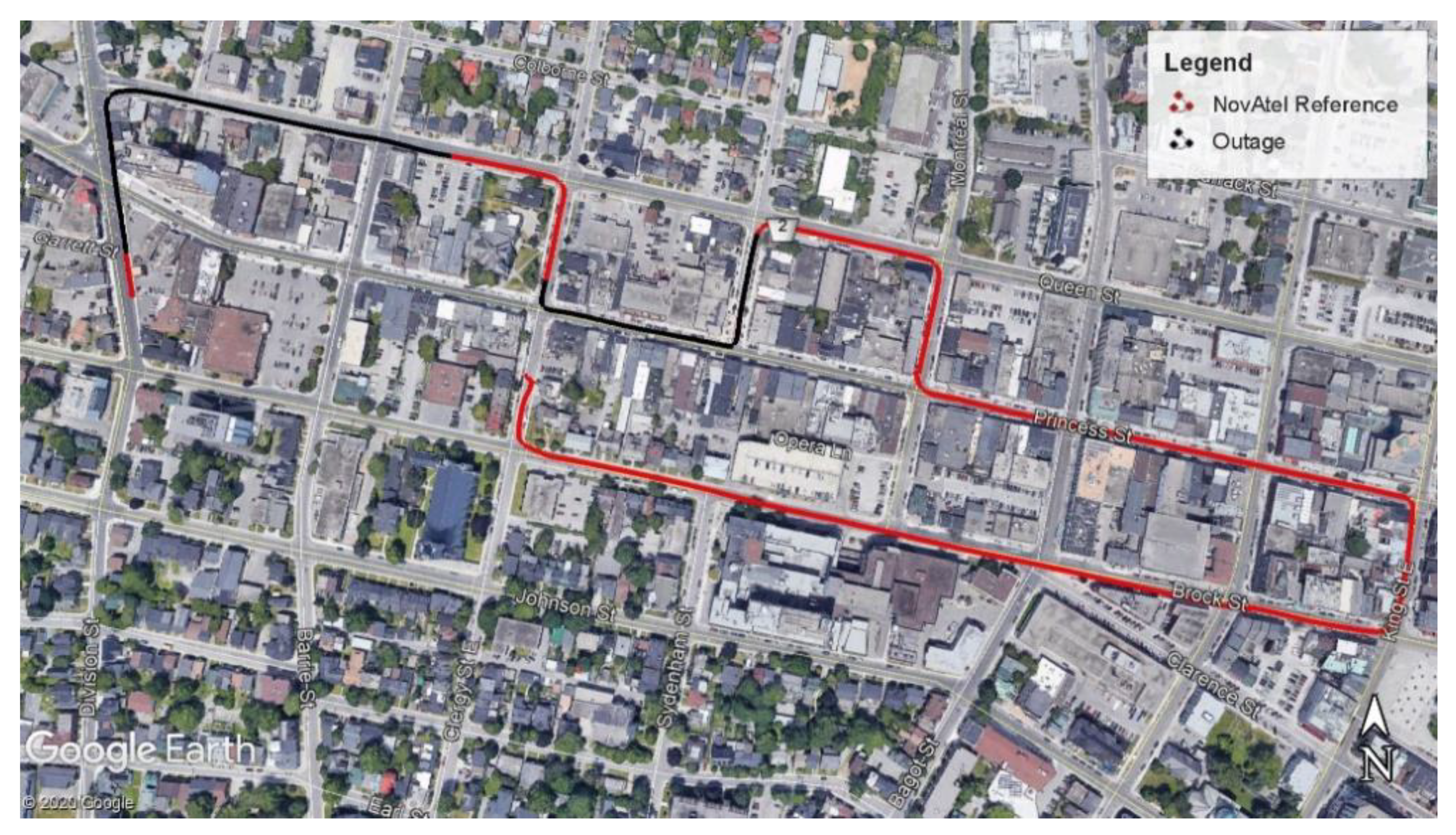
4.1.1. First Road Trajectory

The first trajectory was performed in the city of Kingston, Ontario, Canada, which is considered as a suburban environment as low-mid rise buildings characterize it. The trajectory was conducted in the afternoon around 4 pm on 23 May 2018. It lasted for 17 min and was 2.25 km in length. Due to the infrastructure of the city, and there is hardly any place with extended GNSS coverage. Therefore, two artificial outages were introduced in a post-processing mode to evaluate the performance over different scenarios. Figure 14 shows the full trajectory highlighting the simulated outages chosen to assess the proposed LiDAR/RISS navigation solution.

The first simulated outage shown in Figure 15, lasted for 80 s, and covered a distance of 380 m, passing through a four-way intersection and one sharp turn. Figure 15 presents the results from the LiDAR/RISS solution, the 3D-RISS standalone, and the NovAtel reference solution.

The 3D-RISS standalone resulted in an RMS error of 7.8 m, while the LiDAR/RISS resulted in an RMS error of 4.6 m, which is a 41% improvement. Moreover, the 3D-RISS resulted in a 2D maximum error of 11.87 m, while the LiDAR/RISS showed a slight improvement to 11 m, which is a 7.3% improvement. The deviation over the 380 m traveled was 2.05% for the 3D-RISS, while the LiDAR/RISS was only 1.21%. Figure 16 shows the 2D position error over the first simulated outage.

The second simulated outage, as shown in Figure 17, also lasted for 80 s, and traveled a distance of 225 m with two sharp turns and a four-way intersection.

The 3D-RISS standalone resulted in an RMS error of 13.4 m, while the LiDAR/RISS showed an improvement to 1.7 m, which is an 87% improvement. Moreover, the 2D maximum error in the 3D-RISS was 28.03 m, while the LiDAR/RISS showed considerable improvement to 3.37 m, which is an 88% improvement in the 2D maximum error. The deviation over the 225 m outage, the 3D-RISS deviated 12.45%, while the LiDAR/RISS only deviated 1.5%. The LiDAR/RISS was able to produce an overall better performance compared to the 3D-RISS. Figure 18 shows the 2D position error in meters over the second simulated outage.

As observed in Figure 18, the 3D-RISS deviates from the reference solution due to dynamics introduced in the ($w_z$). However, it is observed that between the seconds 61 to 74, the 3D-RISS standalone solution has a lower 2D position error than the LiDAR/RISS. This observation has led to the motivation of using the 3D-RISS standalone in the switching algorithm, which was explained in Section 3. As the 3D-RISS is given an appropriate initial point, it can perform for a short period without drifting, and this will further be illustrated the second trajectory.

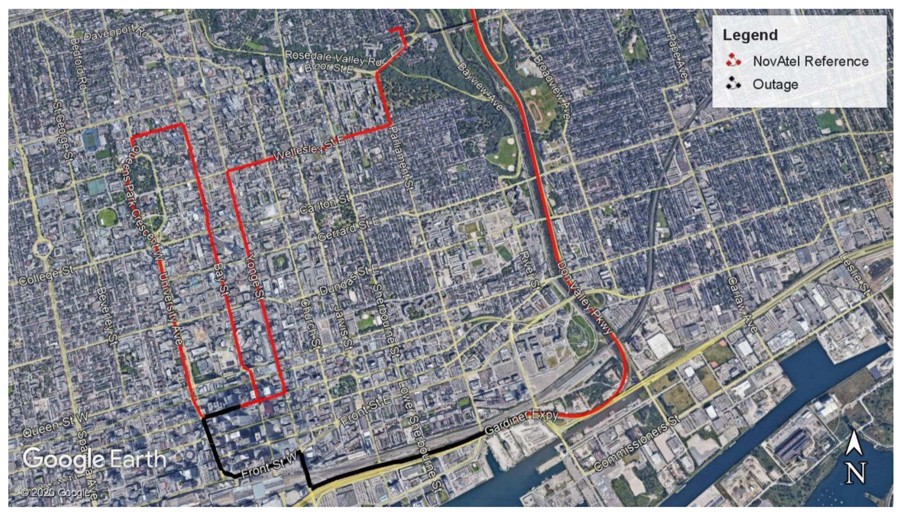
4.1.2. Second Road Trajectory

The second road trajectory was done in a dense urban area environment. It was conducted in the city of Toronto, Ontario, Canada, which is considered a challenging urban area in which the GNSS signal frequently suffers from total blockage and multipath. Therefore, this is considered the main challenge for the proposed MSS and how it can operate in various environments with different scenarios. The trajectory was conducted around noon on 13 June 2018. It lasted for 1 h and 14 min and was 24.4 km in length. Figure 19 shows the trajectory highlighting the scenario selected. The scenario selected started with a good signal of GNSS, then the GNSS signal degrades.

The scenario, as shown in Figure 19, lasted for 9 min and 45 s and covered a distance of 1.98 km. The scenario starts at the highway, where a direct line of sight with the GNSS satellites was established, and the GNSS provided a reliable result. Then, leaving the highway through an exit and facing a stop sign where we took a right turn into a tunnel. While entering the tunnel, the GNSS signal was lost. Then, coming out of the tunnel, the vehicle encountered an intersection and a red traffic light. The car then took a sharp left at the intersection, where the downtown area began to form with high-rise buildings on each side. After that, the vehicle faced a straight road with two traffic lights. Then, at the second traffic light, a slight right turn was made into a straight road until a traffic light where the vehicle took a right turn at the traffic light. Figure 20 shows the complete selected scenario and the navigation solution between the 3D-RISS, the GNSS, the proposed solution LiDAR/RISS/GNSS, and the reference solution.

The 3D-RISS standalone resulted in an RMS error of 46.37 m, while the proposed MSS showed a massive improvement to 16.28 m, which is a 64% improvement in the RMS error value. Moreover, the 3D-RISS standalone resulted in a 2D maximum error of 121.8 m, while the MSS showed considerable improvement to 40 m, which is a 67% improvement in the 2D maximum error value. Also, the deviation along the distance traveled for the standalone 3D-RISS was 6% compared to the MSS of only 2%. Figure 21 shows the 2D position error in meters, highlighting the switching between the systems.

LiDAR/RISS/GNSS does not imply a positioning solution from the three sensors at the same time. However, it is an overall positioning solution toggling between the sensors according to the switching criteria. The algorithm worked on switching between the LiDAR, the GNSS and the 3D-RISS standalone as follows:

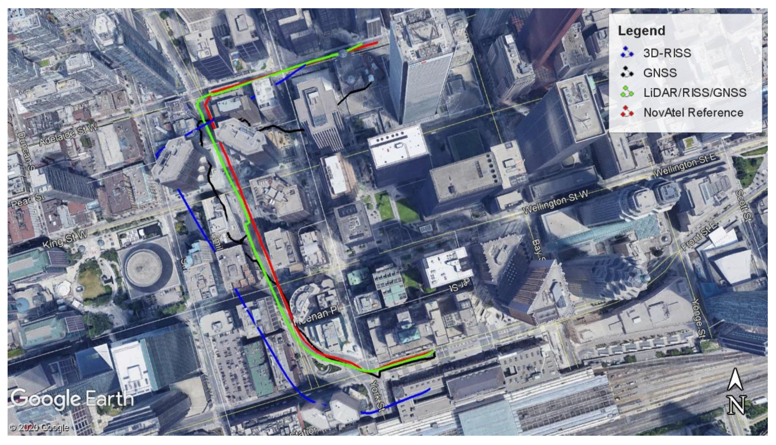
• For the first 147 s, the algorithm was using the GNSS to provide updates in the EKF as it was an open sky environment with good satellite geometry, as shown in Figure 22 from the GDOP values.
• After that, for the next 111 s, the algorithm switched to the LiDAR to provide the measurement updates as the ICP’s RMSE has a low value. As the GDOP values in Figure 22 have spiked as it lost all the GNSS satellites while entering the tunnel. Also, observed in Figure 23 that the SD of the 3D-position begins to increase in value.
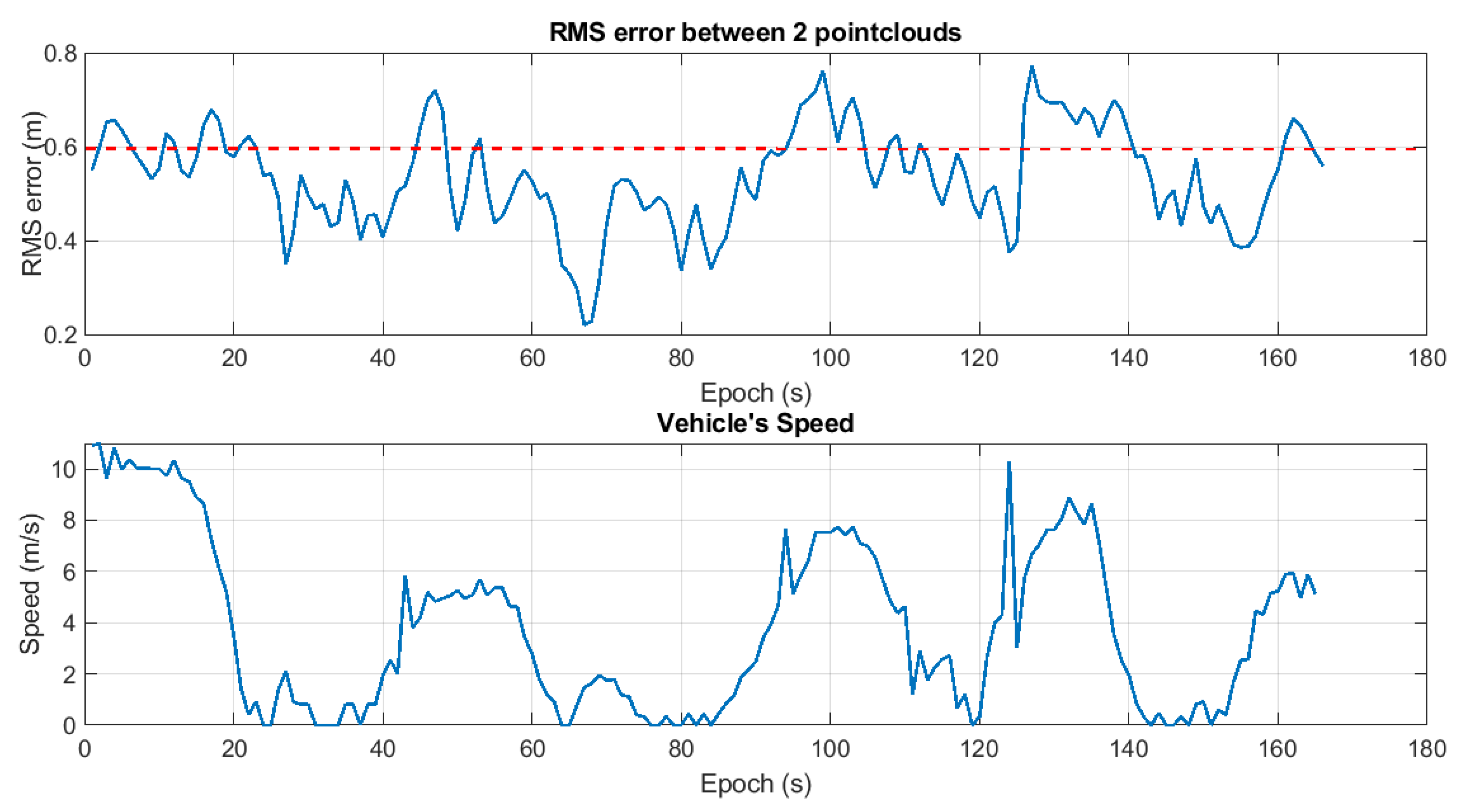
• Then, for the next 80 s, the algorithm switched to the 3D-RISS standalone to provide a navigation solution as the RMS error in the ICP was increasing, as shown in Figure 24.
• Finally, when relying only on the 3D-RISS solution, when a sharp turn is detected by the ($w_z$), as shown in Figure 25, it is switched back to the LiDAR. Therefore, for the last 247 s, the switching criteria will check the GDOP and SD of the GNSS and will find them unsuitable for toggling to the GNSS. Therefore, it will use the LiDAR to provide the measurement updates for the system. As observed in Figure 22 and Figure 23, the GDOP and the SD of the 3D-position provided by the GNSS are still high, which is the reason why we did not rely on the GNSS to provide the measurement updates.

To further explain the scenario, Figure 26 shows the beginning of the chosen scenario. The scenario begins on the highway, where a clear line of sight with the satellites is present, and the GNSS signal provides a reliable solution. The GNSS reliability can be verified from the measurements in Figure 22 and Figure 23. However, as the vehicle exits the highway, the GNSS measurements become unreliable. Also, as observed in Figure 26, the standalone 3D-RISS begins to drift as the vehicle starts exiting the highway.

Figure 27 shows the LiDAR taking the place of the GNSS in providing the measurement updates in the EKF. As shown in Figure 24, the RMSE of the ICP is decreasing as we exit the highway and moving on lower speeds. Therefore, the LiDAR/RISS takes over from the RISS/GNSS at the exit of the highway, then to a right turn where the car enters the tunnel. Inside the tunnel, the vehicle is faced with a stalled car, and from this point, the 3D-RISS starts to drift. However, the LiDAR with the stopping criterion proposed to stop the registration when the vehicle’s speed is lower than the specified threshold of 1 m/s. The LiDAR still provides excellent accuracy and does not drift until the vehicle reaches the traffic light and then takes a left turn. After the left turn, due to the glass panels on the buildings, the LiDAR/RISS solution begins to drift.

The LiDAR/RISS solution began to drift when nearing buildings with large glass panels in the front. When the RMS error of the ICP is above the set threshold, this indicates the LiDAR is beginning to drift. Therefore, the algorithm checks the ($w_z$) of the IMU if it is within the specified range, as shown in Figure 25. So, the algorithm switches to the 3D-RISS standalone to provide the navigation solution. The last valid update of the LiDAR/RISS is used as an initial point for the 3D-RISS. As illustrated in Figure 28, the 3D-RISS takes over for 80 s while the LiDAR registration is working in the background. The switching algorithm keeps monitoring the ($w_z$) of the IMU until it detects that the value is below or above the specified range, as shown in Figure 25. Then, the algorithm switches to back the LiDAR when it finds that the GDOP and the SD of 3D-position from GNSS have high values that correspond to unreliable GNSS measurements.

Figure 27 shows the final part of the scenario, where the LiDAR/RISS provides a solution for 250 s. Monitoring the GDOP values and SD of the 3D-position provided by the GNSS in Figure 22 and Figure 23, the GNSS still does not provide a reliable solution. Moreover, the 3D-RISS standalone at this point due to the sensor error accumulation drifts far away from the solution. The LiDAR/RISS, however, provides a robust, reliable solution in urban areas. As shown in Figure 29, the vehicle passed three traffic lights making a right turn at the last one. After the right turn, as shown in Figure 21, the 2D-position error increases at the end. This increase was due to the large glass panels on the buildings. Therefore, this is the part where the algorithm will detect the increase in the RMS error of the ICP and act accordingly. To either switch to the standalone 3D-RISS or the GNSS.

The previous results and analysis indicate that the proposed MSS mitigates the 3D-RISS drift during the GNSS outage period. Moreover, the MSS provides an overall reliable navigation solution due to its capability of switching between different systems.

5. Conclusions

In conclusion, the work done in this paper introduced an integration scheme of the LiDAR/RISS/GNSS to provide a navigation solution for land vehicles in challenging GNSS environments. Moreover, a switching criterion is proposed to select among the sensors to provide an overall robust navigation solution in different scenarios. The performance of the proposed MSS is assessed based on two different trajectories in two different environments.

The first trajectory conducted in a suburban environment, which is why we introduced an artificial GNSS outage to assess the performance of the LiDAR/RISS integration. It was observed that in an 80-second outage, the LiDAR/RISS showed an improvement over the 3D-RISS standalone. Over two simulated outages without the aid of GNSS, the LiDAR/RISS showed an improvement of 41% and 87% percent, respectively. Also, the LiDAR/RISS provided only a 1% deviation over the distance traveled on both outages while the 3D-RISS standalone showed a 2.05% and a 12.45% deviation, respectively.

The second trajectory, conducted in a downtown area with high rise buildings and crowded areas. As the GNSS signals are faced with multipath and shadowing, the switching algorithm was created to toggle between the LiDAR and GNSS in aiding the INS. The switching algorithm used the GDOP value, the number of satellites, and the SD of the 3D-position provided by the GNSS. Also, the RMS error of the ICP along with the value of the ($w_z$) from the IMU. Over a 10-min outage, the system switched between the RISS/GNSS system to the LiDAR/RISS to the 3D-RISS standalone to accommodate different scenarios and provide a robust and reliable navigation solution for land vehicles. The LiDAR/RISS/GNSS showed a significant improvement over the 3D-RISS standalone by 64%. Furthermore, the total distance traveled was 2 km, and the deviation of the MSS was 2% compared to the 3D-RISS, which was a 6% deviation over the traveled distance.

References

1. Wang, K.; Teunissen, P.J.G.; El-Mowafy, A. The ADOP and PDOP: Two Complementary Diagnostics for GNSS Positioning. J. Surv. Eng. 2020, 146, 04020008. [Google Scholar] [CrossRef] [Green Version]
2. Georgy, J.; Noureldin, A.; Goodall, C. Vehicle Navigator Using a Mixture Particle Filter for Inertial Sensors/Odometer/Map Data/GPS Integration. IEEE Trans. Consum. Electron. 2012, 58, 544–552. [Google Scholar] [CrossRef]
3. Peshekhonov, V.G. Gyroscopic navigation systems: Current status and prospects. Gyroscopy Navig. 2011, 2, 111. [Google Scholar] [CrossRef]
4. Binder, Y.I. Dead Reckoning Using an Attitude and Heading Reference System Based on a Free Gyro with Equatorial Orientation. Gyroscopy Navig. 2017, 8, 104–114. [Google Scholar] [CrossRef]
5. Li, T.; Zhang, H.; Gao, Z.; Niu, X.; El-Sheimy, N. Tight Fusion of a Monocular Camera, MEMS-IMU, and Single-Frequency Multi-GNSS RTK for Precise Navigation in GNSS-Challenged Environments. Remote Sens. 2019, 11, 610. [Google Scholar] [CrossRef] [Green Version]
6. Noureldin, A.; Karamat, T.; Georgy, J. Fundamentals of Inertial Navigation, Satellite-Based Positioning and Their Integration; Springer: Berlin, Germany, 2013; pp. 297–313. [Google Scholar]
7. El-Wakeel, A.S.; Osman, A.; Zorba, N.; Hassanein, H.S.; Noureldin, A. Robust Positioning for Road Information Services in Challenging Environments. IEEE Sens. J. 2020, 20, 3182–3195. [Google Scholar] [CrossRef]
8. Iqbal, U.; Okou, A.F.; Noureldin, A. An Integrated Reduced Inertial Sensor System—RISS/GPS for Land Vehicle. In Proceedings of the 2008 IEEE/ION Position, Location and Navigation Symposium, Monterey, CA, USA, 5–8 May 2008; pp. 1014–1021. [Google Scholar] [CrossRef]
9. Balid, W.; Tafish, H.; Refai, H.H. Intelligent Vehicle Counting and Classification Sensor for Real-Time Traffic Surveillance. IEEE Trans. Intell. Transp. Syst. 2018, 19, 1784–1794. [Google Scholar] [CrossRef]
10. Veronese, L.d.; Badue, C.; Cheein, F.A.; Guivant, J.; de Souza, A.F. A Single Sensor System for Mapping in GNSS-denied environments. Cogn. Syst. Res. 2019, 56, 246–261. [Google Scholar] [CrossRef]
11. Rusinkiewicz, S.; Levoy, M. Efficient Variants of the ICP Algorithm. In Proceedings of the Third International Conference on 3-D Digital Imaging and Modeling, Quebec, QC, Canada, 28 May–1 June 2001; pp. 145–152. [Google Scholar] [CrossRef] [Green Version]
12. Mohamed, S.A.S.; Haghbayan, M.; Westerlund, T.; Heikkonen, J.; Tenhunen, H.; Plosila, J. A Survey on Odometry for Autonomous Navigation Systems. IEEE Access 2019, 7, 97466–97486. [Google Scholar] [CrossRef]
13. Zhang, S.; Guo, Y.; Zhu, Q.; Liu, Z. Lidar-IMU and Wheel Odometer Based Autonomous Vehicle Localization System. In Proceedings of the 2019 Chinese Control and Decision Conference (CCDC), Nanchang, China, 3–5 June 2019; pp. 4950–4955. [Google Scholar] [CrossRef]
14. Khalife, J.; Ragothaman, S.; Kassas, Z.M. Pose Estimation with Lidar Odometry and Cellular Pseudoranges. In Proceedings of the 2017 IEEE Intelligent Vehicles Symposium (IV), Los Angeles, CA, USA, 11–14 June 2017; pp. 1722–1727. [Google Scholar]
15. Chang, L.; Niu, X.; Liu, T.; Tang, J.; Qian, C. GNSS/INS/LiDAR-SLAM Integrated Navigation System Based on Graph Optimization. Remote Sens. 2019, 11, 1009. [Google Scholar] [CrossRef] [Green Version]
16. ABrandt; Gardner, J.F. Constrained Navigation Algorithms for Strapdown Inertial Navigation Systems with Reduced Set of Sensors. In Proceedings of the 1998 American Control Conference, ACC (IEEE Cat. No. 98CH36207), Philadelphia, PA, USA, 26 June 1998; Volume 3, pp. 1848–1852. [Google Scholar]
17. Iqbal, U.; Georgy, J.; Abdelfatah, W.F.; Korenberg, M.; Noureldin, A. Enhancing Kalman Filtering–based Tightly Coupled Navigation Solution Through Remedial Estimates for Pseudorange Measurements Using Parallel Sascade Identification. Instrum. Sci. Technol. 2012, 40, 530–566. [Google Scholar] [CrossRef]
18. Aboutaleb, A.; Ragab, H.; Nourledin, A. Examining the Benefits of LiDAR Odometry Integrated with GNSS and INS in Urban Areas. In Proceedings of the 32nd International Technical Meeting of the Satellite Division of The Institute of Navigation (ION GNSS+ 2019), Miami, FL, USA, 16–20 September 2019. [Google Scholar]
19. Bogoslavskyi, I.; Stachniss, C. Efficient Online Segmentation for Sparse 3D Laser Scans. Photogramm. Fernerkund. Geoinf. 2016, 85, 41–52. [Google Scholar] [CrossRef]
20. Guo, Y.; Wang, H.; Hu, Q.; Liu, H.; Liu, L.; Bennamoun, M. Deep Learning for 3D Point Clouds: A Survey. arXiv 2019, arXiv:1912.12033. [Google Scholar]
21. Velodyne LiDAR PUCK LITETM Datasheet. Available online: https://velodynelidar.com/products/puck-lite/ (accessed on 20 January 2020).
22. Zermas, D.; Izzat, I.; Papanikolopoulos, N. Fast Segmentation of 3D Point Clouds: A Paradigm on LiDAR Data for Autonomous Vehicle Applications. In Proceedings of the 2017 IEEE International Conference on Robotics and Automation (ICRA), Singapore, 29 May–3 June 2017; pp. 5067–5073. [Google Scholar] [CrossRef]
23. NovAtel. OEM4 Family User Manual-Volume 1. Available online: https://forsbergpnt.com/wp-content/uploads/2016/04/OEM4-user-manual-Rev-19.pdf (accessed on 1 June 2020).
24. Abosekeen, A.; Noureldin, A.; Karamt, T.; Korenberg, M. Comparative Analysis of Magnetic-Based RISS using Different MEMS-Based Sensors. In Proceedings of the 30th International Technical Meeting of the Satellite Division of The Institute of Navigation (ION GNSS+ 2017), Portland, OR, USA, 25–29 September 2017. [Google Scholar]
25. Ublox. ANN-MS Active GPS Antenna Manual. Available online: https://www.u-blox.com/en/docs/UBX-15025046 (accessed on 8 May 2020).
26. NovAtel. NovAtel SPAN-SETM Manual. Available online: https://www.novatel.com/assets/Documents/Manuals/om-20000124.pdf (accessed on 8 May 2020).
27. NovAtel. NovAtel SPAN IMU-CPT Manual. Available online: https://www.novatel.com/assets/Documents/Papers/IMU-CPT.pdf (accessed on 8 May 2020).
28. Schneider, A. GPS Visualizer. Available online: www.gpsvisualizer.com (accessed on 8 May 2020).
Figure 1. 3D-RISS Mechanization Block Diagram.
Remotesensing 12 02323 g001
Figure 2. Point Cloud Preparation Flowchart.
Remotesensing 12 02323 g002
Figure 3. Ego Vehicle Points Labeled in Red in the Point Cloud.
Remotesensing 12 02323 g003
Figure 4. Ground Points Labeled in Yellow in the Point Cloud.
Remotesensing 12 02323 g004
Figure 5. Arbitrary Points A and B with respect to the Sensor at O.
Remotesensing 12 02323 g005
Figure 6. Point Cloud Clustered Based on Euclidean Distance.
Remotesensing 12 02323 g006
Figure 7. (a) Raw Point Cloud with red circles highlighting the most distinctive points that are removed; (b) Denoised Point Cloud.
Remotesensing 12 02323 g007
Figure 8. (a) Normal Point Cloud; (b) Downsampled Point Cloud.
Remotesensing 12 02323 g008
Figure 9. Root Mean Squared (RMS) error versus Speed Plot Highlighting the Average RMS error Calculated.
Remotesensing 12 02323 g009
Figure 10. LiDAR/RISS/GNSS System Architecture.
Remotesensing 12 02323 g010
Figure 11. Switching Algorithm Flowchart.
Remotesensing 12 02323 g011
Figure 12. (a) Minivan Used for the Trajectories; (b) Sensors Mounted on the Rooftop.
Remotesensing 12 02323 g012
Figure 13. Sensor Setup on the Testbed.
Remotesensing 12 02323 g013
Figure 14. First Trajectory Highlighting the Simulated Outages.
Remotesensing 12 02323 g014
Figure 15. Navigation Solution for 3D-RISS, LiDAR/RISS, and NovAtel Reference during Simulated GNSS Outage 1, First Trajectory.
Remotesensing 12 02323 g015
Figure 16. 2D Position Error for Simulated Outage 1, First Trajectory.
Remotesensing 12 02323 g016
Figure 17. Navigation Solution for 3D-RISS, LiDAR/RISS, and NovAtel Reference during Simulated GNSS Outage 2, First Trajectory.
Remotesensing 12 02323 g017
Figure 18. 2D Position Error for Outage 2, First Trajectory.
Remotesensing 12 02323 g018
Figure 19. Second Trajectory Highlighting the Scenario.
Remotesensing 12 02323 g019
Figure 20. Navigation Solution for 3D-RISS, GNSS, LiDAR/RISS/GNSS, and NovAtel Reference During the Selected Scenario.
Remotesensing 12 02323 g020
Figure 21. 2D Position Error for Second Trajectory Scenario.
Remotesensing 12 02323 g021
Figure 22. GDOP Values Before, During, and After the Scenario Highlighting the Switching Between the Systems.
Remotesensing 12 02323 g022
Figure 23. The SD of the 3D-position Provided by the GNSS Before, During, and After the Scenario Highlighting the Switching Between the Systems.
Remotesensing 12 02323 g023
Figure 24. The RMSE of the ICP Calculated in the Selected Scenario.
Remotesensing 12 02323 g024
Figure 25. The (wz)measured by the IMU in the Selected Scenario.
Remotesensing 12 02323 g025
Figure 26. Navigation solution for 3D-RISS, GNSS, LiDAR/RISS/GNSS, and NovAtel reference at the Beginning of the Scenario.
Remotesensing 12 02323 g026
Figure 27. Navigation solution for 3D-RISS, GNSS, LiDAR/RISS/GNSS, and NovAtel Reference During the Scenario (First Switch).
Remotesensing 12 02323 g027
Figure 28. Navigation solution for 3D-RISS, GNSS, LiDAR/RISS/GNSS, and NovAtel Reference During the Scenario (Second Switch).
Remotesensing 12 02323 g028
Figure 29. Navigation solution for 3D-RISS, GNSS, LiDAR/RISS/GNSS, and NovAtel reference during the Scenario (Third Switch).
Remotesensing 12 02323 g029