Article

A Sensitivity Study of POD Using Dual-Frequency GPS for CubeSats Data Limitation and Resources

1
School of Earth and Planetary Sciences, Curtin University, GPO Box U1987, WA 6845 Perth, Australia
2
Department of Mechanical and Aerospace Engineering, West Virginia University, 1306 Evansdale Drive, PO Box 6070, Morgantown, WV 26506-6070, USA
*
Author to whom correspondence should be addressed.
Remote Sens. 2020, 12(13), 2107; https://doi.org/10.3390/rs12132107
Submission received: 10 June 2020 / Revised: 26 June 2020 / Accepted: 27 June 2020 / Published: 1 July 2020
(This article belongs to the Special Issue Positioning and Navigation in Remote Sensing)

Abstract

:
Making use of dual-frequency (DF) global navigation satellite system (GNSS) observations and good dynamic models, the precise orbit determination (POD) for the satellites on low earth orbits has been intensively investigated in the last decades and has achieved an accuracy of centimeters. With the rapidly increasing number of the CubeSat missions in recent years, the POD of CubeSats were also attempted with combined dynamic models and GNSS DF observations. While comprehensive dynamic models are allowed to be used in the postprocessing mode, strong constraints on the data completeness, continuity, and restricted resources due to the power and size limits of CubeSats still hamper the high-accuracy POD. An analysis of these constraints and their impact on the achievable orbital accuracy thus needs to be considered in the planning phase. In this study, with the focus put on the use of DF GNSS data in postprocessing CubeSat POD, a detailed sensitivity analysis of the orbital accuracy was performed w.r.t. the data continuity, completeness, observation sampling interval, latency requirements, availability of the attitude information, and arc length. It is found that the overlapping of several constraints often causes a relatively large degradation in the orbital accuracy, especially when one of the constraints is related to a low duty-cycle of, e.g., below 40% of time. Assuming that the GNSS data is properly tracked except for the assumed constraints, and using the International GNSS Service (IGS) final products or products from the IGS real-time service, the 3D orbital accuracy for arcs of 6 h to 24 h should generally be within or around 1 dm, provided that the limitation on data is not too severe, i.e., with a duty-cycle not lower than 40% and an observation sampling interval not larger than 60 s.

Graphical Abstract

1. Introduction

Combining strong dynamic models and observations of global navigation satellite system (GNSS) collected onboard, the processing strategies used for the low Earth orbit (LEO) reduced-dynamic precise orbit determination (POD) have been intensively investigated in the last decades [1,2,3,4,5]. Compared to the dynamic orbits based on the dynamic models only and the kinematic orbits based on the GNSS observations only, the reduced-dynamic orbit determination has the advantage that it is more robust against model deficiencies for the former case, and possible data constraints, e.g., data in-continuity for the latter case. Following the need for the POD by a range of applications, such as the studies in the Earth gravity field [6,7], the atmospheric sounding [8], the altimetry [9], and the Interferometric Synthetic Aperture Radar (InSAR) [10], the LEO orbital accuracy based on undifferenced GNSS observations can reach a few centimeters [11,12], and even better at mm-level in case of baseline processing for formation-flying [12,13,14]. For undifferenced POD, the highest accuracy is often realized in postprocessing mode applying good dynamic models, precise GNSS satellite orbits, and clocks, and under the condition that the GPS dual-frequency phase and code data are tracked and collected with a good continuity and completeness. The antenna attitude information is often well monitored by extra sensors like star cameras and inertial measurement unit (IMU), and eventually will be used to correctly apply the antenna sensor offsets, the antenna phase centre offsets (PCOs), and variations (PCVs) [15].
The number of CubeSat missions has dramatically increased in this decade. By April 2020, there are over 1000 CubeSats successfully launched into their low earth orbits [16]. In addition to educational purposes, CubeSats are nowadays also used for the demonstration of new technologies and scientific researches [17,18]. Compared to large or medium LEO satellites, the CubeSats are mostly cost-effective and occupy a much smaller size and weight, i.e., typically from below 1 kg (0.25U) to more than 20 kg (12U). This often leads to smaller battery volume and smaller size of the solar panels. In addition to the two-line elements (TLEs), other sensors like sun sensors and magnetometers have been used for orbit determination of CubeSats with relatively low accuracy, i.e., at km-level [19]. In the case of higher positioning accuracy requirements, the GNSS-based processing has been demonstrated as a useful method for the CubeSat POD, for which successful postprocessed position fix was achieved with a meter-level accuracy [20]. While the onboard positioning normally utilizes simplified dynamic models due to the limitation of the computational load [21,22], the data postprocessing allows the usage of comprehensive dynamic models and the estimation of enough additional dynamic parameters to compensate remaining model deficiencies. However, even for the postprocessing mode, strongly constrained satellite size and power need to be shared among all sensors onboard. The capacity for data tracking, storage, and transfer is thus restricted, which limits the accuracy of orbit determination. The GNSS satellites may not be able to be fully tracked continuously due to these limitations, which could yield a duty-cycle smaller than 100% [20,21,23], and lead to fewer data available for the processing and more ambiguities to be set up. The size of the data collected between each data dump could also be limited [20]. The collected GNSS observations are most likely to be temporarily stored onboard and transferred back to the ground processing centre (GPC) every orbital cycle or a few cycles during a limited ground contact time, while information of tasks other than positioning is required to be stored and transferred at the same time. This may implicitly limit the GNSS data amount during the downlink. Due to these constraints and the potential limit on computational load in case of the real-time onboard processing, a relatively low sampling rate might be preferable for CubeSat POD, or low in general but only high in specific areas [24]. Furthermore, one may need to prepare for a low number of tracked satellites in case of assigning channels for the purpose of initial signal acquisitions [20] and in case of improper data tracking due to possible antenna control problems, which will be discussed later in this section.
In addition to the data continuity and availability, other information required for the POD may also be limited for CubeSat missions. Due to the limitation of the CubeSats in terms of their size, power, and capacity to install extra sensors, the antenna attitude information may not be well measured, estimated, documented, and transferred back to the GPC with sufficient details. For example, due to power management needs, the IMU under its own high-accuracy experiment [25] onboard the CubeSat Simulation To Flight-1 (STF-1), investigated by NASA’s Katherine Johnson Independent Verification and Validation (IV&V) Facility and West Virginia University [21,26], was unable to be activated during the GNSS data collection. Depending on the latency requirements of the CubeSat orbits, the high-accuracy GNSS satellite orbits and clocks might not be available for the processing, e.g., the international GNSS service (IGS) final products [27,28], which has a latency of 12–18 days. As explained in [11], this could lead to dramatic accuracy differences already in case of good data continuity and availability, mainly due to the decreased sampling rates of the satellite clocks. Moreover, instead of processing orbits with long arcs of 24 h or 12 h (which accounts for about 16 and 8 orbital cycles for an orbital period of 1.5 h), rapid processing may also be used to compute the orbit with shorter arcs of several hours. While some conditions mentioned above may not significantly influence the orbital accuracy when individually being considered, large degradation of different levels could happen when several conditions happen together. Therefore, at the planning phase of a CubeSat mission, it is important to assess the orbital accuracy under different scenarios, so that one can properly compromise between the limits on diverse resources and the expected orbital accuracy.
The GNSS-based orbit determination of small satellites is often performed with single-frequency signals [23,24,29,30], which leads to an accuracy of decimeters to meters depending on the data availability and the dynamic models used. In recent years, to enable a higher POD accuracy, the usage of dual-frequency code and phase GPS data has been attempted and planned in CubeSat missions, even for a multi-constellation scenario [31]. Having dual-frequency phase and code observations at hand, the first-order ionospheric delays, which amounts to about 99% of the total ionospheric delays [32], can be eliminated by forming the ionosphere-free (IF) combination instead of the group and phase ionospheric correction (GRAPHIC) combination, which is often formed in the single-frequency case involving both the code and phase signals. While having the second frequency should theoretically enables better POD accuracy, a higher challenge for data tracking, storage, and transfer is also associated with the use of the dual-frequency GNSS in CubeSat missions. In addition to the planned constraints on diverse resources, the actual data collection of the dual-frequency CubeSat missions may not fulfil the expectation due to the lower robustness compared to the large LEO satellites. As an example, Figure 1 shows the real data condition of the 3U CubeSat STF-1 experimented by NASA’s Katherine Johnson IV&V Facility and West Virginia University, which was expected to collect dual-frequency GPS data with a duty-cycle of 100% during a specific 12 h period. The actual data condition, however, did not meet the expectation, possibly due to the lack of the antenna attitude control. Due to the limitations in the antenna system, reports of short data pieces and frequent cycle slips, which hampers the high-accuracy POD, can also be found for the triple-CubeSat CanX-2 [20]. As such, not only for the planning purpose but also to get prepared for the possible sub-optimal real data collection, investigations of the CubeSat POD accuracy with diverse constraints on data and resources are important. A proper compromise is very possibly needed between the limiting resources, the suboptimal data conditions, and the requirements on orbital accuracy.
For the dual-frequency CubeSat POD, which is the focus of this study, it was pointed out by previous studies that the discontinuity of the observation data with a low duty-cycle may significantly degrade the orbital accuracy in both the real-time and the postprocessing modes [21,33]. In this study, we restrict focus on postprocessing reduced-dynamic dual-frequency CubeSat POD, which relieves the strong constraints of the computational load onboard the CubeSat and allows for the usage of good dynamic models. In the experiments of CanX-2 [20] and STF-1 [21], geodetic grade receivers NovAtel OEM4-G2 and OEM615 tracking dual-frequency GPS signals were mounted onboard the CubeSats. With the expectation that in future CubeSat missions, dual-frequency measurements can be properly tracked in each duty-cycle by geodetic receivers with a mean average satellite number of at least 5 to 6, this study performs a sensitivity analysis of different limitations on the data availability, continuity, resources, latencies, and arc lengths with respect to the orbital accuracy. The overlapping effect of different constraints is investigated, and a compromise between these factors and the orbital accuracy is discussed. In addition to CubeSats, the analysis should also benefit the POD of other small satellites that need to bare similar constraints on data, power, and resources.

2. Processing Strategy

In this study, the final LEO orbits (where CubeSats are classified as LEO) are postprocessed following the reduced-dynamic LEO processing scheme of the Bernese GNSS Software V5.2 [34]. After correcting the antenna PCOs, PCVs, and the offsets between the antenna reference point (ARP) and the satellite center-of-mass (CoM), the determined final orbit in this study is referred to the satellite CoM. For the sensitivity analysis purpose, the final reduced-dynamic orbits are produced assuming different observation sampling rates, duty cycling, varying mean number of satellites by changing the elevation mask as will be explained in the next section, arc lengths, using different types of the IGS products, with and without the antenna attitude information. The processing procedure can generally be summarized in the following steps, which is also given in Figure 2 as a flow diagram:
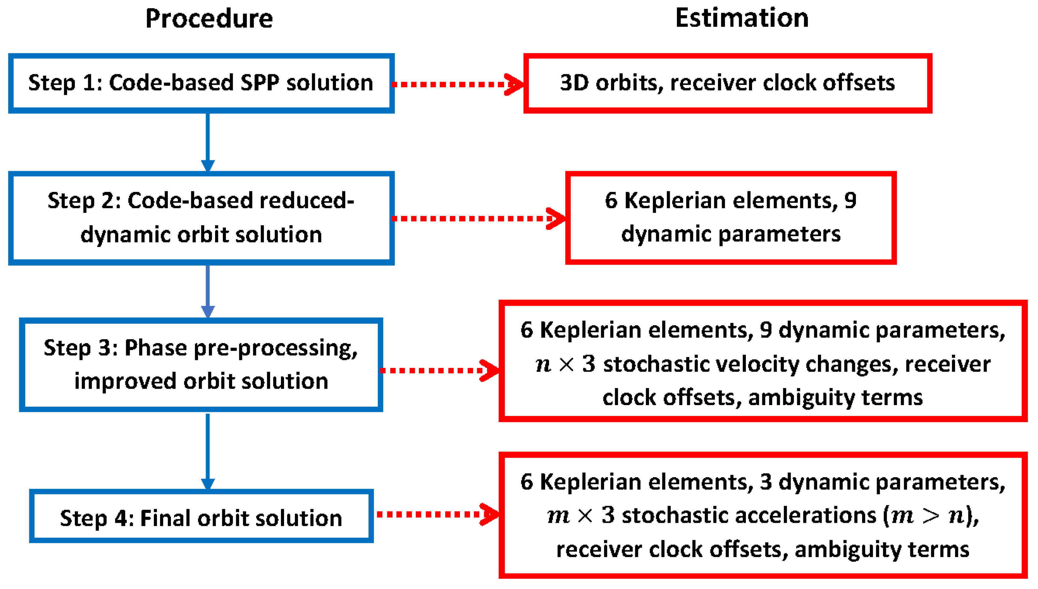
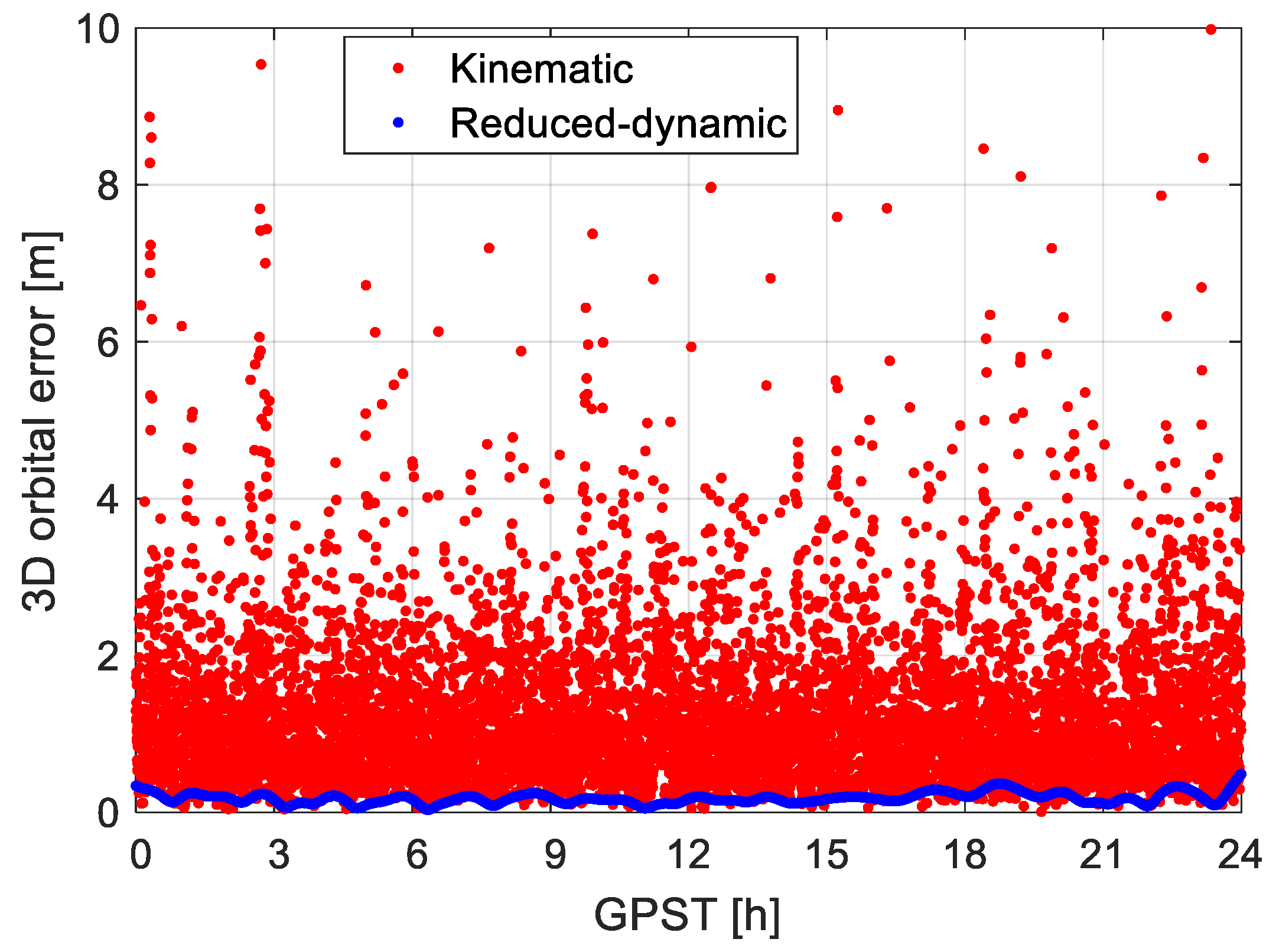
  • Compute kinematic orbits using single point positioning (SPP) employing the IF combination of the code observations. These kinematic orbits, denoted as vector r ^ K , are discrete and have an accuracy of meters.
  • Computation of the code-based reduced-dynamic orbits. The reduced-dynamic orbits are computed with accelerations based on a series of gravitational and nongravitational terms, such as the Earth gravitational terms, the Earth tidal terms, the gravitational attraction from the sun, moon, and other planets, as well as the general relativistic term. Note that mis-modeled effects like the solar radiation pressure and the air drag will be largely absorbed by the estimated dynamic parameters and the stochastic velocity changes or accelerations set up later in the processing [35]. Details of the processing and the dynamic models are given in Table 1. Making use of the kinematic code orbits from the first step, the six Keplerian elements at the initial condition (the semi-major axis of the orbit, the orbital eccentricity, the inclination of the orbital plane, the right ascension of the ascending node, the argument of perigee, and the argument of latitude at the initial condition), and a remaining part of the dynamic models are estimated with a batch least-squares adjustment, which includes at this step nine flight-oriented dynamic parameters. These estimable dynamic parameters contain three constant terms ( a R 0 , a S 0 , and a W 0 ) and six periodic terms ( a R C , a S C , a W C , a R S , a S S , and a W S ) in the radial (R), along-track (S) and cross-track (W) directions. The total acceleration a can then be distributed into the term a 0 , which is assumed known by applying the models given in Table 1, and an additional dynamic term a d y n that is to be adjusted:
    a = a 0 + a d y n ,
    With
    a d y n = a R e R + a S e S + a W e W ,
    a R = a R 0 + a R C cos ( U ) + a R S sin ( U ) ,
    a S = a S 0 + a S C cos ( U ) + a S S sin ( U ) ,
    a W = a W 0 + a W C cos ( U ) + a W S sin ( U ) ,
    where e R , e S , and e W represent the unit vectors in the radial, along-track, and cross-track directions, respectively. U denotes the satellite argument of latitude. The code-based kinematic orbits r ^ K obtained from the first step are used as observations to adjust the 15 parameters mentioned above in a least-squares sense. The linearized observation equation at the epoch t i can be formulated as:
    E ( r ^ K r ^ 0 ) = [ A r k ,   A r d ] [ x k ,   x d ] T ,
    where r ^ 0 is the a priori orbit vector obtained based on numerical integration on hand the a 0 , and the a ^ d y n and the Keplerian elements estimated from the last iteration. The vectors x k and x d contain the increments of the six Keplerian elements and the nine dynamic parameters, respectively, and the design matrices A r k and A r d contain the partial derivatives of the position vectors with respect to x k and x d . The partial derivatives are computed with numerical integration of the variational equations [36,37]. E is the expectation operator. The reduced-dynamic orbit can be interpolated for time epochs with higher sampling rates and produced for periods with data gaps. In this study, all orbits are resampled into time epochs with 10 s sampling interval for assessment, regardless of which duty-cycles and observation sampling rates are applied in the processing.
3.
Phase preprocessing and orbit improvements. This step preprocesses the raw phase observations to detect cycle slips and mark bad observations. The preprocessing goes through several iterations to improve the LEO orbit quality. The orbit improvement is realized through estimation of stochastic velocity changes [38] in addition to the 15 parameters mentioned in the second step, and is performed in a least-squares adjustment making use of the IF combination of the phase observations. One set of the stochastic velocity changes is considered in each predefined time interval, e.g., every 15 min. The linearized phase observation equation at the epoch t i can be expressed as:
E ( Δ φ I F ) = [ A l k , A l d , A l v ] [ x k , x d , x v ] T + c × Δ t r + λ I F N I F ,
With
λ I F = c f 1 + f 2 ,
N I F = f 1 2 λ 1 N 1 f 2 2 λ 2 N 2 c ( f 1 f 2 ) ,
where ∆φIF represents the observed-minus-computed (O-C) term of the IF phase observations. c and Δtr denote the speed of light and the receiver clock error, respectively. λj, fj, and Nj represent the wavelength, the frequency, and the ambiguity on frequency j (j = 1, 2), respectively. Note that NIF is not an integer. The receiver clock error is estimated epoch-wise independently, and the ambiguity is assumed constant before the detection of a cycle slip. Note that new ambiguities are setup for estimation at the beginning of each round of duty cycling. xv stands for the vector containing all stochastic velocity changes in the RSW directions from the first to the current epoch and note that xv is constrained to zero with a predefined a priori standard deviation. The design matrices Alk, Ald, and Alv contain the partial derivatives of the O-C terms with respect to the xk, xd, and xv, respectively. To be estimated are the vector [xk,xd,xv]T, the receiver clock offset Δtr, and the term NIF. Note that very little code observations are used to avoid the problem of matrix singularity between the receiver clock offset and the ambiguity terms. Note that the ambiguities on L1 and L2 are not attempted to be fixed in this study.
4.
Generation of final orbits. With the preprocessed phase observations, the six Keplerian elements, the three constant dynamic parameters ( a R 0 , a S 0 , and a W 0 ) are estimated together with stochastic accelerations in the RSW directions. The accelerations are set up in shorter time intervals compared to those in Step 3. The linearized phase observation equation is thus formulated as:
E ( Δ φ I F ) = [ A l k , A l d 0 , A l a ] [ x k , x d 0 , x a ] T + c × Δ t r + λ I F N I F ,
where x d 0 and x a denote the increment vector of the three constant dynamic parameters and all the stochastic accelerations from the first to the current epoch, respectively. x a is constrained to zero with a predefined a priori standard deviation (selected as 5 ×   10 9 m/ s 2 in all the three directions based on the default setting for GRACE satellites in the Bernese software, as real data from the GRACE Follow-on mission is used for test purposes in this study, which will be explained later. This value may vary for satellites of other missions). A l d 0 and A l a correspond to the partial derivatives of the phase O-C terms with respect to the x d 0 and x a , respectively. Note that very little code observations are used to avoid singularity mentioned above.
In this study, the data from the LEO satellite of the GRACE Follow-on mission [43], the GRACE FO-1, which continuously tracked dual-frequency code and phase GPS observations on L1 and L2, are used for different scenarios simulating conditions with limited data and resources on 22 August 2018. For the purpose of consistency, the processed orbits are differenced with the best-case scenario in this study (as the reference for comparison), i.e., the phase-based reduced dynamic orbits with a duty-cycle of 100%, an observation sampling interval of 10 s, an elevation mask of 5 degrees (default setting in Bernese for LEO processing), using the IGS final products and processed in a 24 h arc. The use of our best-case scenario as a reference for comparing different tested cases is justified by comparing it with the reference orbits provided by the Jet Propulsion Laboratory (JPL) [44] for the same day, where good consistency with a 3-dimentional (3D) root-mean-squared error (RMSE) of below 2 cm was achieved. Nevertheless, it should be noted that in this study, the 3D RMSE computed under different scenarios refer to the accuracy difference compared with the best-case scenario, but not the absolute orbital accuracy. Note that for LEO missions, independent technics like the satellite laser ranging (SLR) and the K-band ranging (KBR) are often utilized to validate the accuracy of reference orbits. As a large number of variants with respect to different observation sampling rates, duty-cycles, satellite numbers, latencies, availability of the attitude information, and arc lengths are tested, this study does not attempt to study long-term variation of results. As a consistency check, the POD results of the best-case scenario from 14 to 21 August 2018 were compared with the JPL reference orbits, and no significant difference from those of the test day in this study can be observed, i.e., at a few millimeters. As such, we consider the simulations based on the test day are representative.

3. Orbit Determination under Different Scenarios

As a start point of our analysis, let us look at the results of code-based processing and see the impact of using a reduced-dynamic model. Figure 3 shows the 3D positional errors of the kinematic orbits (red) based on the code observations on P1 and P2 forming the IF combination (Step 1 in Section 2), and when computing the same data with the reduced-dynamic orbits (blue, Step 2 in Section 2) for GRACE FO-1 for the tested 1 day of data. As complete dual-frequency CubeSats data for a long period needed in our analysis are currently not available, the data from a typical LEO satellite that may share similar orbit conditions with CubeSats, in this study GRACE FO-1, were used for simulation of the best-case scenario of the CubeSat processing [33]. For the tested LEO satellite, the dual-frequency GPS data are tracked in a complete and continuous manner with an observation sampling interval of 10 s. A duty-cycle of 100% and a mean satellite number of about 9 above the elevation mask of 5 degrees were available for the processing of a daily arc using the IGS final products. The 3D RMSE of the code-based kinematic (Step 1 in Section 2) and reduced-dynamic orbits (Step 1 in Section 2) amount to about 1.6 m and 0.2 m, respectively, which clearly shows the value of employing strong dynamic models. When reducing the data availability and continuity, the accuracy of the reduced-dynamic orbit could degrade to the sub-meter level.
For high-accuracy POD, as discussed in Section 2, the code-based orbits are only used as the a priori orbits for the phase processing. Therefore, in the rest of the sections, the sensitivity analysis will focus on the final phase-based reduced-dynamic orbits.

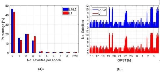
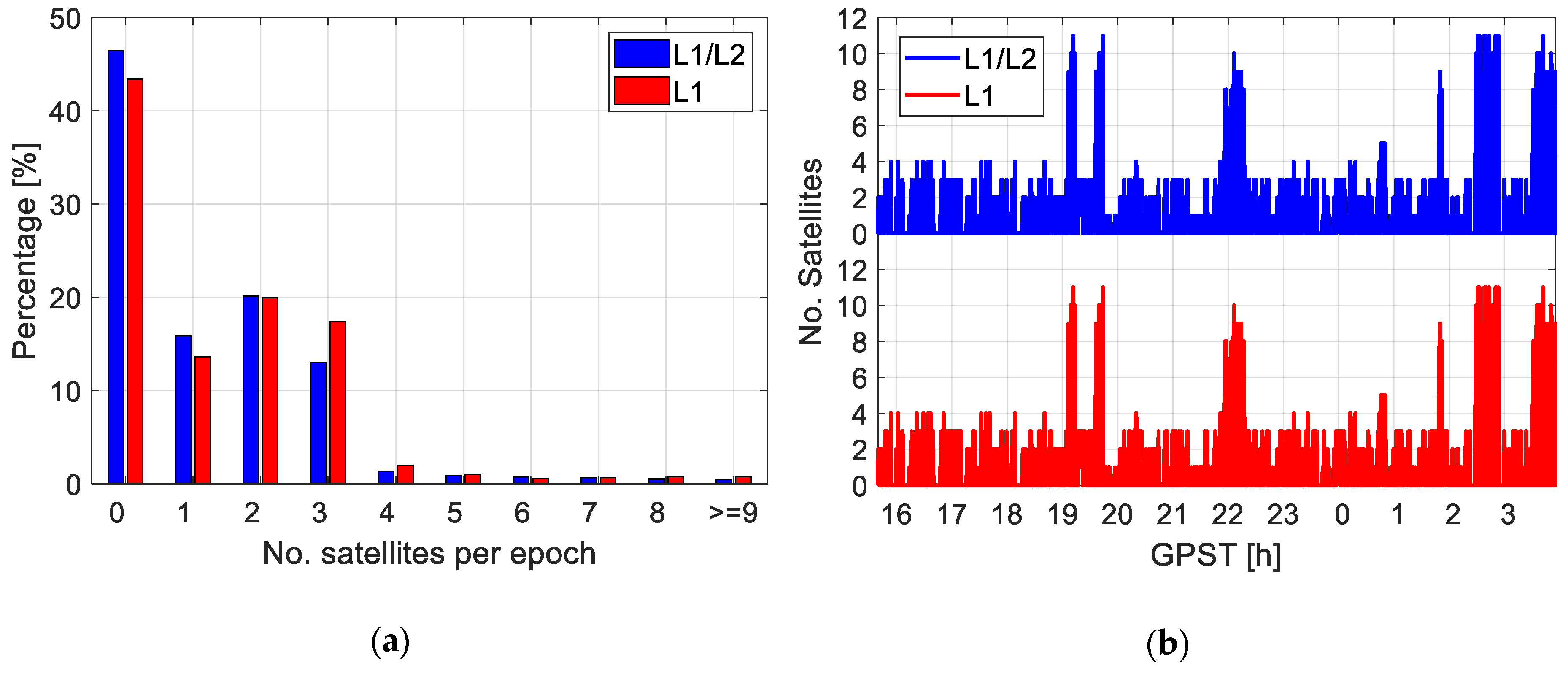
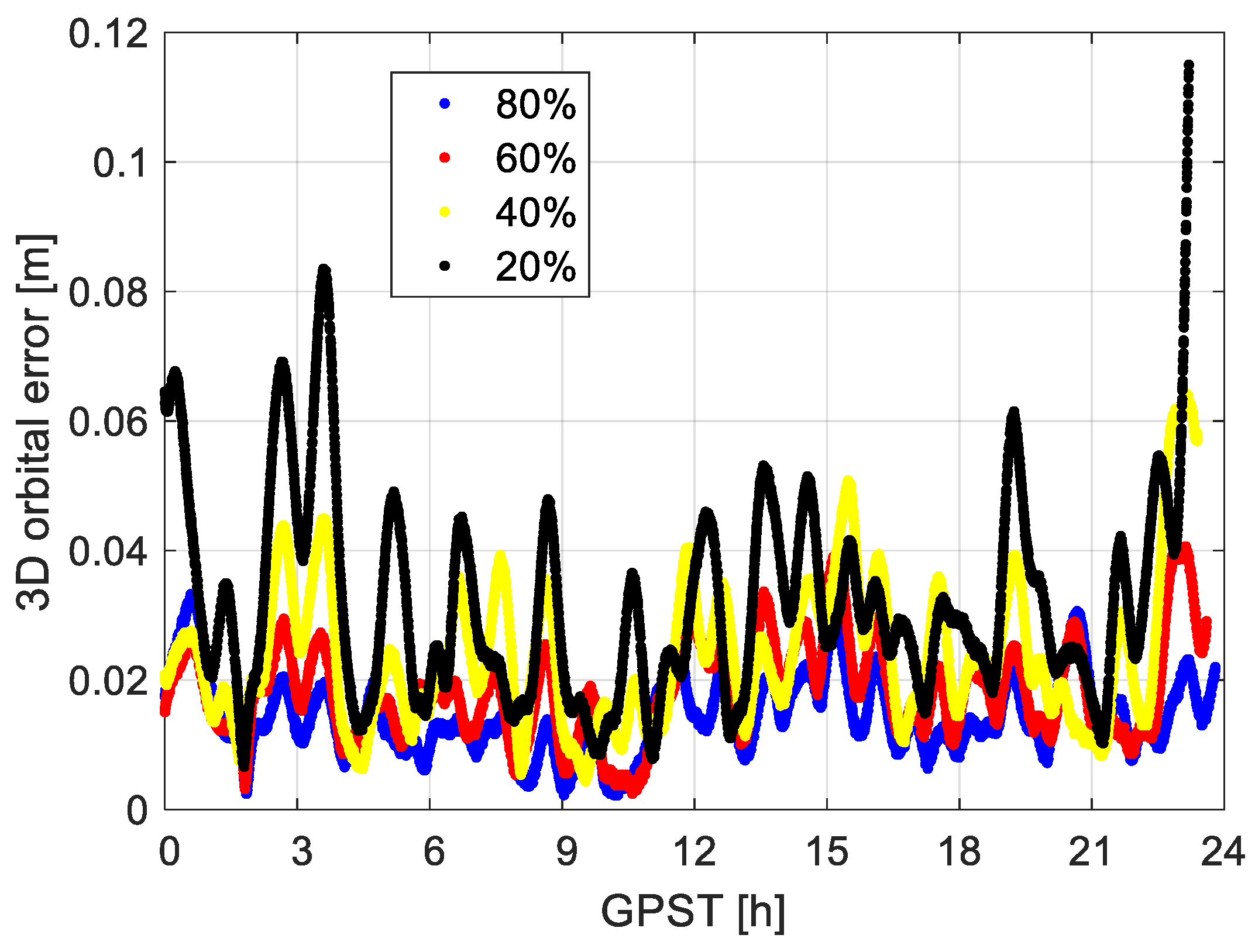
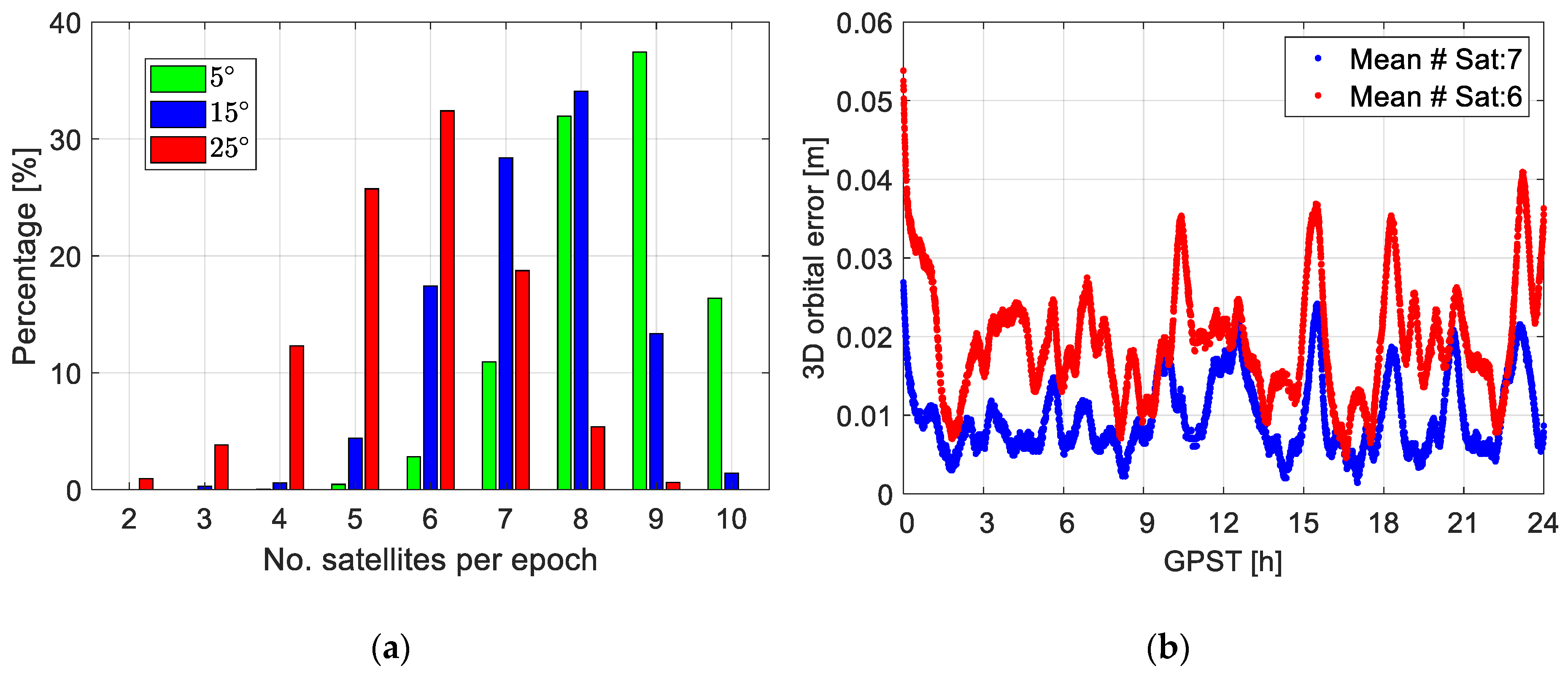
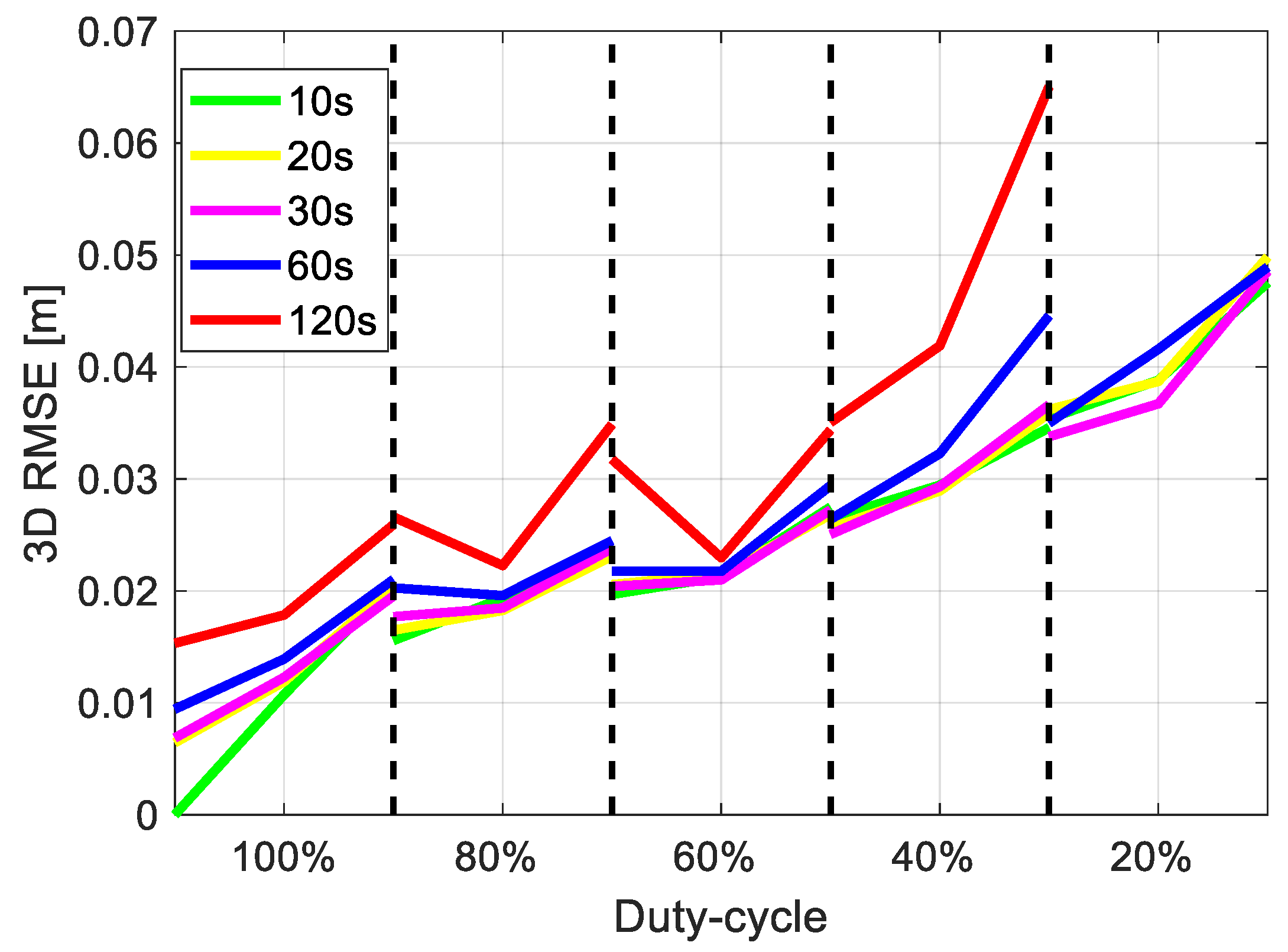
3.1. Duty Cycling and Satellite Numbers

As mentioned before, due to the constraints of the CubeSats on the power, the data storage, and the time of active attitude control possibly during the sunlight, the GNSS observations might have breaks, and are collected in pieces of different length [20]. In this study, observation data are assumed to be collected with different duty-cycles, i.e., with the power turned on only for a part of the time. The duty-cycle D is defined here as a percentage of time data was available out of the total time considered. The sensitivity analysis is performed assuming the D varying from 20% to 100%. In our tests, a duty-cycle implies that the data are available in the first 60 × D min of each hour. The 3D orbital errors are shown in Figure 4 with varying D . The observation sampling interval was 10 s. Recall that the phase-based reduced-dynamic orbit with a duty-cycle of 100% was our best-case scenario and was used as the reference for comparison as mentioned in Section 2. The RMSE increases from about 1.6 cm with a D of 80% to about 3.5 cm with a D of 20%. Note that the RMSE is computed from the beginning of the first power-on period to the end of the last power-on period of the test day.
As shown in Figure 1 and discussed in [19], the number of satellites that can be properly tracked (at least for the P1 and P2 observations) by the CubeSat receiver could be lower than expected due to different reasons, such as the antenna stabilization problems or specific channel assignment. Therefore, to resemble this practical issue, a simplified approach is performed in this simulation to reduce the number of satellites observed under good conditions by excluding satellites with low elevation angles. The elevation mask is increased from 5 to 25 degrees in the test, resulting in a reduction of the mean satellite number from about 9 to 6 (see Table 2). The Figure 5a illustrates the distribution of the satellite numbers applying different elevation masks for GRACE FO-1 for the test period. A gradual reduction of the satellite numbers can be observed when increasing the elevation mask. The percentile of valid SPP solutions is reduced correspondingly from nearly 100% to about 83% due to the reduction in redundancy.
Having a duty-cycle of 100%, as shown in Figure 5b, decreasing the number of the received satellites from, e.g., 7 to 6, degrades the RMSE from about 1.1 to 2.1 cm. Note that the case with the mean satellite number of 9 having an elevation mask of 5 degrees is our best-case scenario and is used as the reference for comparison, in other words, the RMSE represent the solution discrepancy between the cases of using 7 or 6 satellites and when using 9 satellites.
Although the differences observed in Figure 4 and Figure 5 are not large, coupling a reduction in the duty-cycle with a reduction in the number of received satellites would cause larger problems. Table 3 shows the 3D RMSE of the orbits applying different duty-cycles and mean satellite numbers, assuming an observation sampling interval of 10 s still. As mentioned earlier, the solution obtained with a duty-cycle of 100% and the mean satellite number of 9 is used as the reference for assessing the solutions by computing their discrepancies. It can be observed that with a duty-cycle equal or above 60%, even when the observed satellites are limited, the RMSE is still below 3 cm. With lower duty-cycles, however, observing all or almost all visible satellites would be essential to maintain a low RMSE at this level. With a duty-cycle of 20%, decreasing the mean satellite number to 6 would increase the RMSE to about 5 cm.

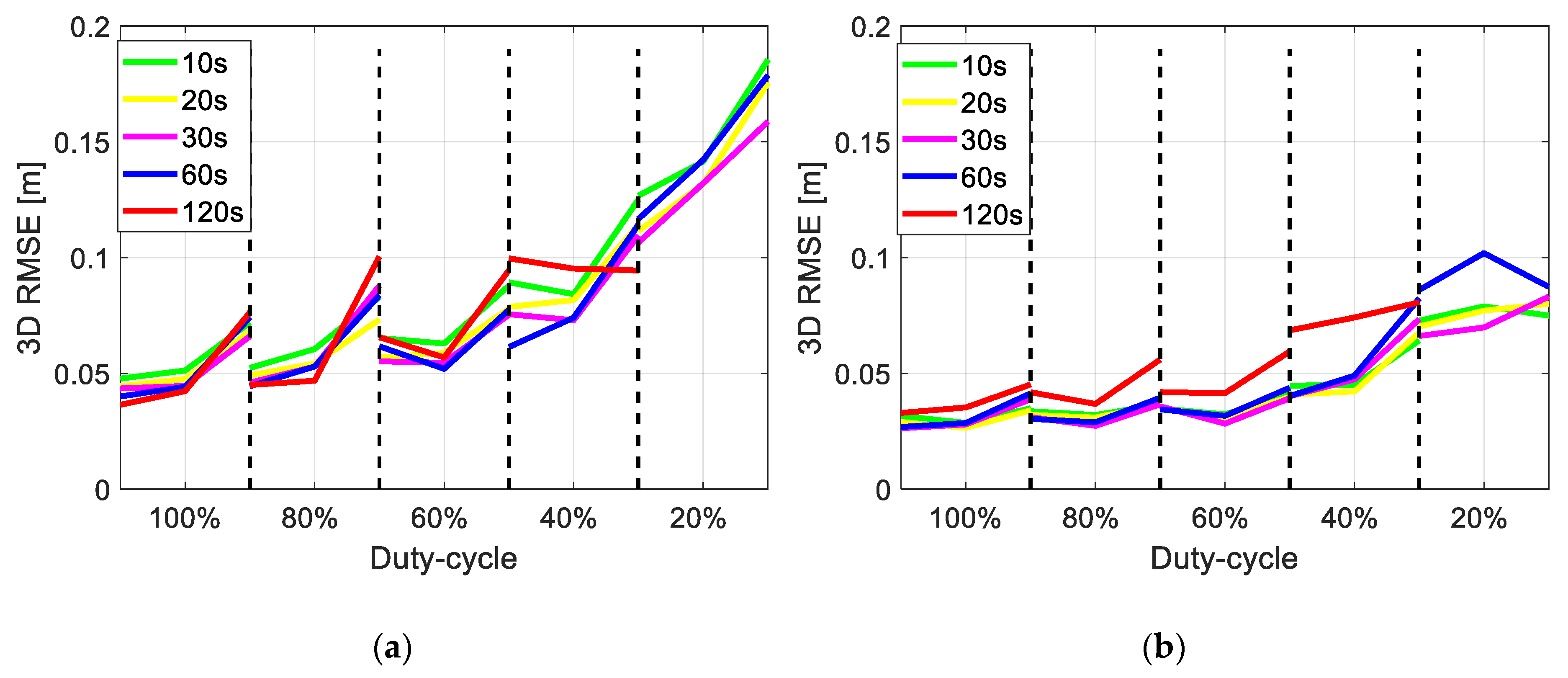
3.2. Sampling Rate of the Observations

In Section 3.1, the GPS observations onboard the LEO satellite with a sampling interval of 10 s were used for producing the reduced-dynamic orbits. Depending on the capacity of the CubeSat missions, the data might need to be stored and transferred to the GPC with a lower sampling rate. A compromise thus needs to be considered between the duty-cycles, the data completeness, and the sampling rate. Figure 6 illustrates the 3D RMSE of the orbits with the sampling interval varying from 10 to 120 s and the duty-cycle varying from 100% to 20%. The cases having mean satellite numbers of 9, 7, and 6 are given between each pair of dashed lines. Recall that the number of satellites is controlled by adjusting the elevation mask (Section 3.1). In the case of a duty-cycle of 20%, the orbits generated with an observation sampling interval of 120 s (red line) are not produced due to the extremely low number of continuous observations in each data patch. Note that all the RMSE are computed based on orbits resampled to 10 s sampling intervals.
From Figure 6 it can be observed that the values in general gradually increase from the left to the right side, i.e., from the cases with good data continuity, completeness, to those with bad data conditions. With less data available for the processing in the Steps 3 and 4 (Section 2), the estimable parameters, including the six Keplerian elements, the additional dynamic parameters, and the stochastic parameters, are determined with lower precision. This results in a lower accuracy of the numerically integrated orbits. At the same time, it can also be observed that the differences between having observation sampling intervals of 10 s (green), 20 s (yellow), and 30 s (magenta) are small. This can be attributed to the 30 s GPS clocks provided in the IGS final products, where interpolation into high-sampled time epochs would introduce biases within a higher percentage of the processing time (to be discussed in the next subsection). Provided that the receiver has a high duty-cycle not lower than 60%, even with a limited number of observed satellites and a high sampling interval of 120 s, the 3D RMSE is still below or around 3 cm. However, with lower duty-cycles, the degradation of the orbit accuracy could be dramatic when the observations are only available with a low sampling rate and when the observed satellites are limited.

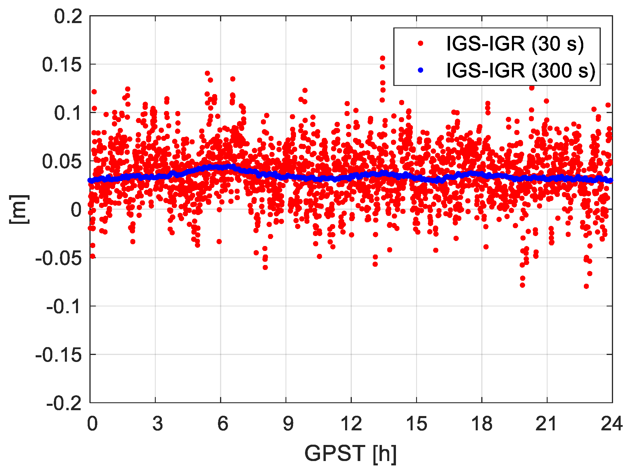
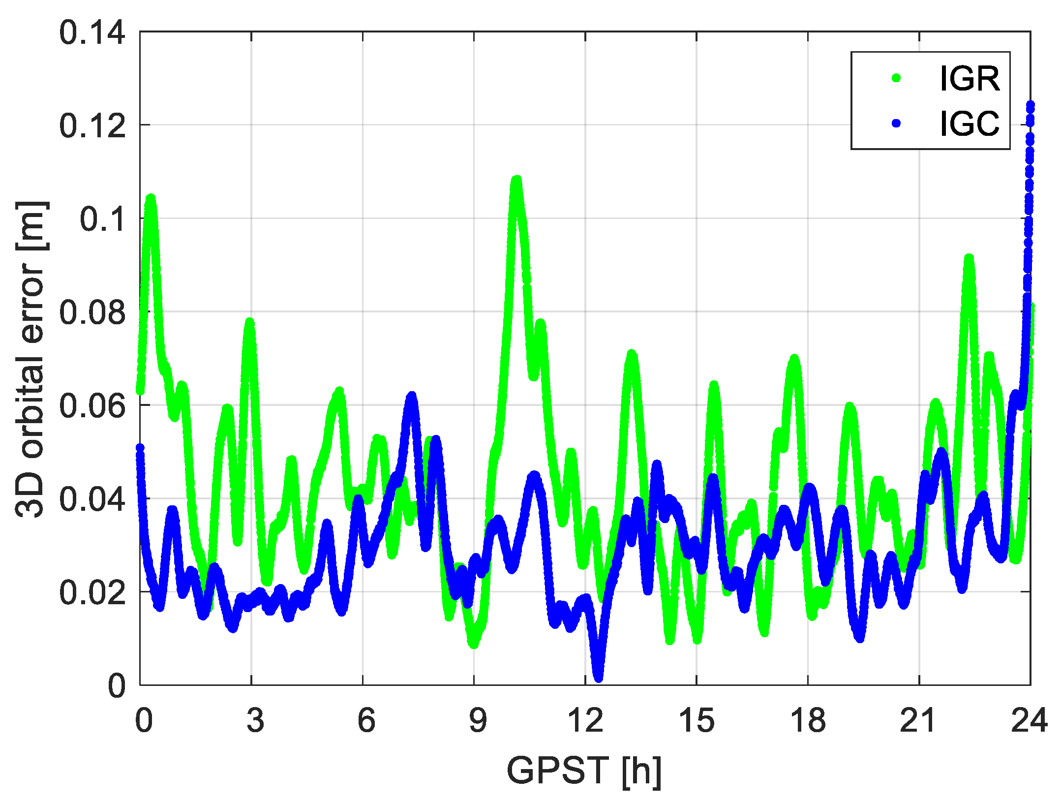
3.3. Latency Applying Different GPS Products

In Section 3.1 and Section 3.2, the IGS final products for GPS satellite orbits and clocks were used for the estimation of the reduced-dynamic orbits. The IGS final products are produced weekly and have a latency of 12 to 18 days. In case that the CubeSat orbits are required within a shorter time, the IGS (or one of its analysis centres) rapid products or products from the IGS real-time service (RTS) [45,46] can be used instead. Table 4 gives the latencies of different IGS products. In this study, the decoded IGS real-time stream IGC01, which is denoted as the IGC products and available at [47], is used for simulation of the scenario retrieving the GPS products in (near)-real-time. Products of the single IGS analysis centers, e.g., the real-time products from the National Centre for Space Studies (CNES), are also of high quality [48]. In this study, for consistency purpose, we used the IGS products of different latencies and satellite clock sampling rates.
Despite the accuracy differences [46,49], from Table 4 it can also be seen that the sampling rate of the IGR satellite clocks is lower than the other two products. In [11], the sampling interval of GPS satellite clock-offset corrections was identified as a limiting factor for the LEO orbital accuracy. This possibly explains the fact that the 3D orbital RMSE using the IGR products are not better than those using the IGC products. Figure 7 shows the differences of the between-satellite clock corrections for G02 and G32 between the IGS final and rapid clocks. The between-satellite clock differences are shown to remove possible inconsistencies between the reference time scales of different products. The blue dots indicate the differences at the given sampling interval of the rapid clocks, i.e., 300 s. The red dots illustrate the differences at a sampling interval of 30 s, where the rapid clocks were linearly interpolated using the nearest epochs to this higher sampling rate. From Figure 7 it can be observed that although the differences are generally at centimeters for the blue dots with the given sampling rate of the rapid clocks, after interpolation, the differences are increased to dm-level (see the red dots). For the test day, the average RMS of the clock differences for all satellites between the IGS and IGR final products, divided by 2 for the between-satellite differencing, amount to about 2 cm. Note that the large pattern of the red dots is caused by the stochastic behaviors of the clocks, and an interpolation over a longer period with a higher-order polynomial does not help to reduce the biases. As an example, interpolation with a quadratic polynomial within each half hour increases the average RMS by several millimeters.
Assuming a duty-cycle of 100%, an observation sampling interval of 10 s, and a mean satellite number of 9, the last column of Table 4 shows the 3D RMSE of the final LEO orbits determined using different IGS products compared with the best-case scenario, i.e., using the IGS final products. A 3D RMSE of several centimeters can be achieved for the IGR and IGC products. This is further illustrated by Figure 8, which shows the time series of the 3D orbital errors applying the IGR and IGC products.
In the case of having limited data available, i.e., with short duty-cycles, limited satellite numbers and sampling rate, the orbital accuracy using the IGR and IGC products would not be as good as shown in Figure 8 anymore. In the case of using the IGR and IGC products, Figure 9 illustrated the 3D RMSE of the difference between phase-based reduced-dynamic orbits and the best-case scenario when applying different duty-cycles, mean satellite numbers, and observation sampling rates. Note that the cases having different satellite numbers (9, 7, and 6) are given between each pair of the dashed lines. Compared to Figure 6 using the IGS final products, the 3D RMSE has generally increased due to the reduced accuracy of the GPS products and the higher sampling interval of the GPS clocks (for IGR products). As discussed for the IGS final products, when using the IGC products (Figure 9b), one can similarly observe that a high observation sampling interval of, e.g., 10 s (green) or 20 s (yellow), is not helpful to reduce the RMSE due to the GPS clock sampling of 30 s. For the cases when using the IGR products (Figure 9a) with a higher GPS clock sampling interval of 300 s (Table 4), no obvious degradation can be concluded even when having an observation sampling interval of 120 s.

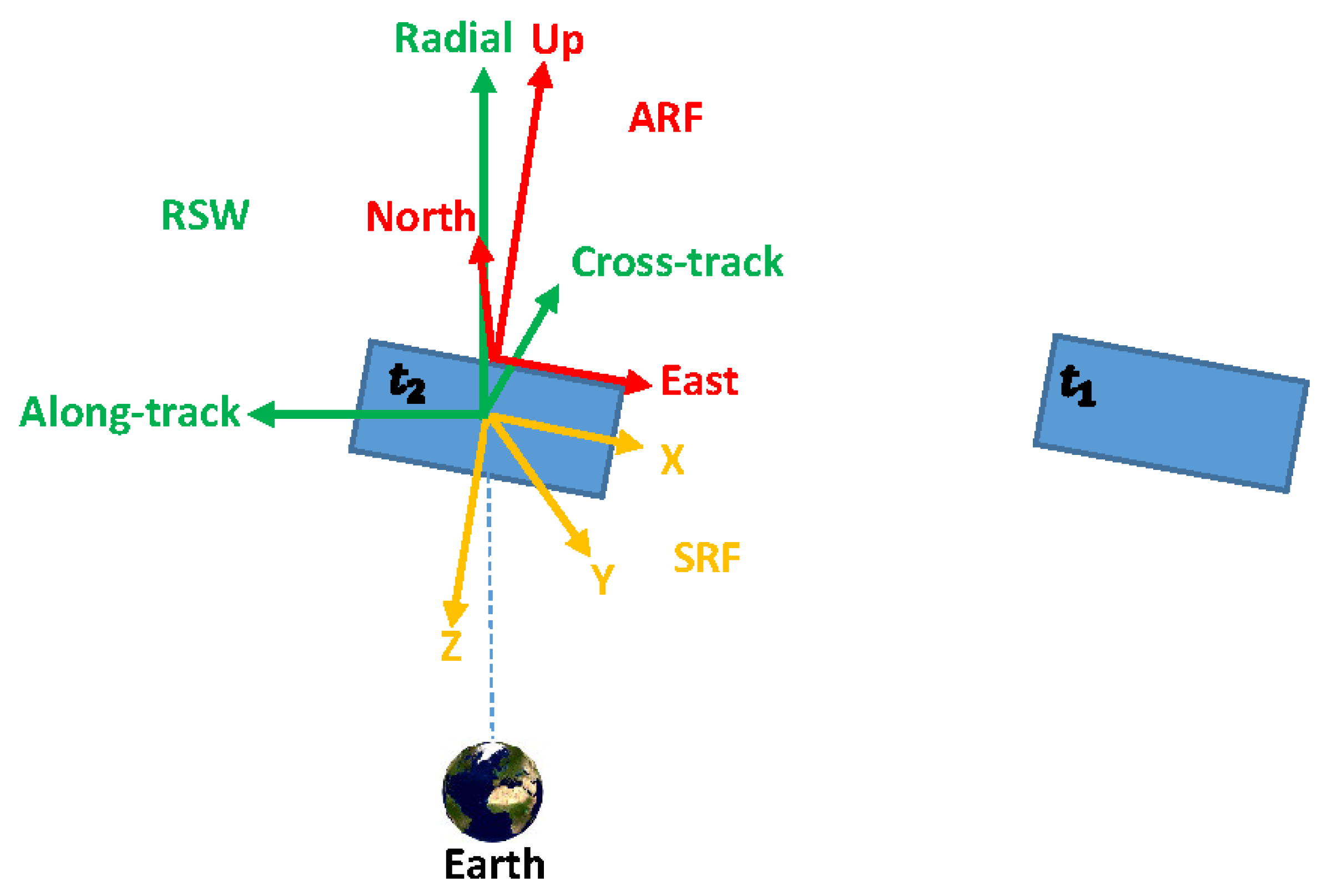
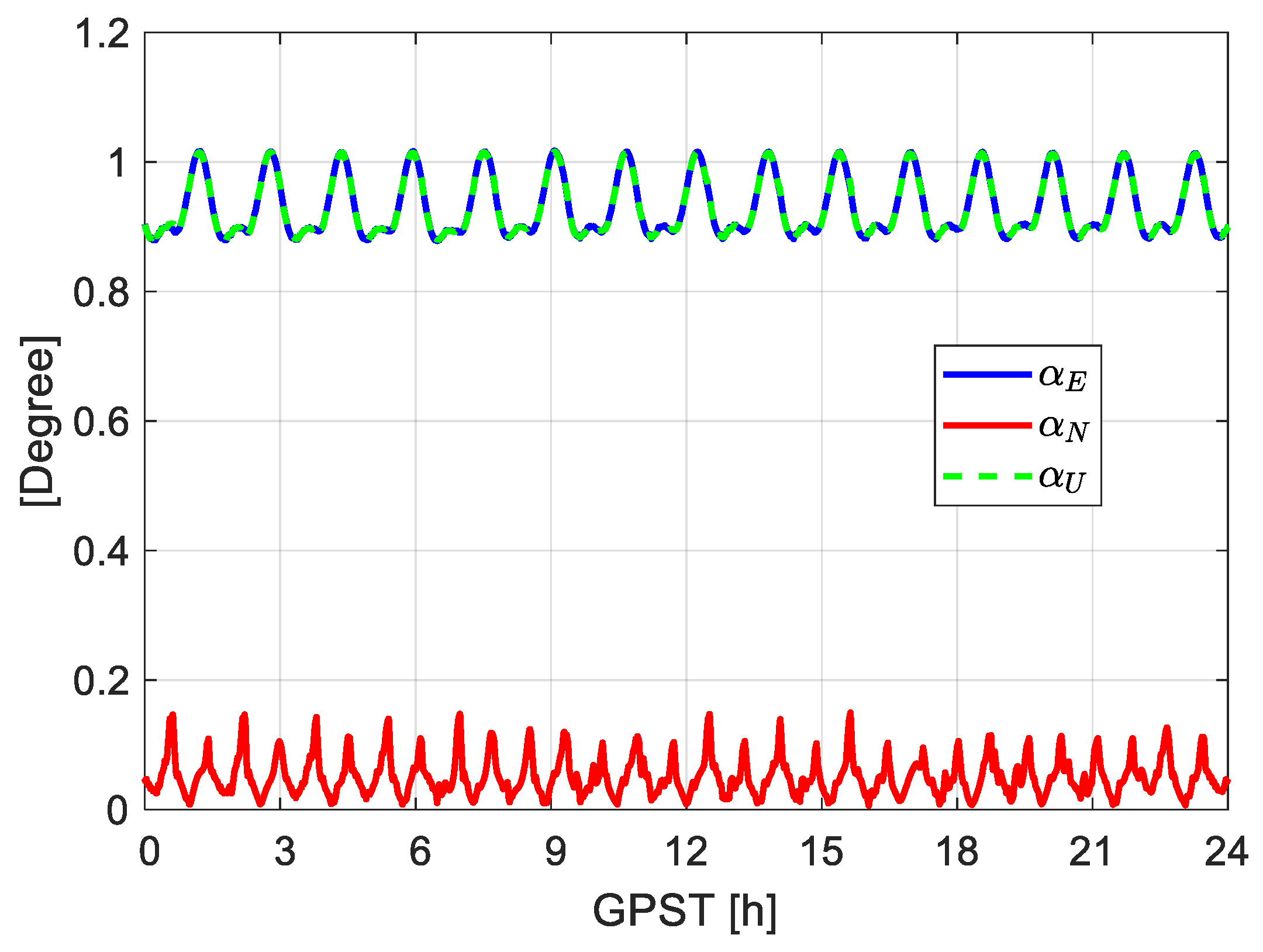
3.4. Antenna Attitude

As shown in the example in Figure 1, it is suspected that the poor data tracking condition is caused by the lack of antenna stabilization. Good antenna stabilization is essential to keep the antenna in a favorable orientation for GNSS tracking, i.e., approximately toward the radial direction. High-accuracy attitude control is expected to be realized also for CubeSats, as found to be feasible in the tests simulating different CubeSat scenarios in [50] and achieved for the CubeSat CanX-2 [20]. Under the condition of appropriate antenna stabilization, the antenna attitude information is often measured by extra sensors like star cameras or IMU on LEO/CubeSats satellites. For CubeSats, however, the limited size and power may limit its capacity to properly measure, store, or transfer the attitude information back to the GPC. As mentioned in Section 1, the data from the IMU onboard the CubeSat STF-1, e.g., was not collected during the GNSS data tracking because of the power allocation, where the IMU used was of a special type tested for a high-accuracy experiment that was carried out at a different time. The attitude information of the satellite (and antenna) is sometimes even ignored in CubeSat simulation studies [21]. Under such circumstances, where no attitude information is available, the antenna attitude could be estimated based on the satellite positions and velocities. Taking the GRACE FO-1 as an example, the antenna was fixed on the satellite and its up direction generally points toward the radial direction from the earth to the LEO satellite. Note that the X-axis in the satellite reference frame (SRF) is here approximately in the anti-flight direction, as GRACE FO-1 is the leading satellite in the test period. Figure 10 depicts the RSW system (green) in the radial, along-track and cross-track directions with the origin in the satellite centre-of-mass, and the antenna reference frame (ARF, red), e.g., for GRACE FO-1, in the north, east, and up (NEU) directions with the origin in the antenna reference point (ARP). To evaluate the differences between the expected and the actual orientations, the angle differences are computed with the help of the east ( e E ) and the opposite along-track ( e S ) unit vectors, the north ( e N ) and the cross-track ( e W ) unit vectors, and the up ( e U ) and the radial ( e R ) unit vectors in the inertial system:
α E = arccos ( e E T e S ) , α N = arccos ( e N T e W ) , α U = arccos ( e U T e R ) .
In Equation (11), the unit vectors e R and e S are calculated based on the satellite position and velocity vectors, and e W completes the left-hand system. As the antenna is fixed on the satellite, the antenna NEU unit vectors e N , e E , and e U are calculated based on the satellite orientations, which are tracked by extra sensors and documented in an attitude file with quaternions. The rotation matrix R S R F transforming from the SRF to the inertial system can be computed with these quaternions [51]. Based on the definition of the SRF as illustrated in Figure 10 in yellow, the e N , e E , and e U can be obtained with:
e E = R S R F [ 1 , 0 , 0 ] T , e N = R S R F [ 0 , 1 , 0 ] T , e U = R S R F [ 0 , 0 , 1 ] T
The angle differences α E , α N , and α U are given in Figure 11. It can be observed that these angle differences are not large. In case that the antenna attitude file is not given, or the attitude information is not accurately documented, one could approximate the antenna orientation using the RSW directions.
Benefiting from the fact that the angle differences between the actual and the expected antenna orientation are small, even without having the attitude information available, differences less than 10 mm can mostly be observed in the final orbits provided that the observation data is complete and continuous (see Figure 12), i.e., with a 3D RMSE amounting to 8 mm. Applying the IGS final products, for other cases with reduced duty-cycles and mean satellite numbers, the differences in the RMSE (referenced to the best-case scenario) with and without applying the attitude file are also mostly at several millimeters. This applies also to the cases when using the IGR and IGC products. This suggests that good attitude control can maintain the POD accuracy even when the attitudes are not properly determined or transferred back to the GPC.

3.5. Length of Arc

The orbital period of a LEO satellite is typically around 1.5 h, depending on its altitude from the Earth’s surface. Taking the GRACE FO-1 as an example, based on the semi-major axis estimated in the final reference orbit, its orbital period is approximately 1 h 34 min 29 s for the test day. A 24 h arc for data analysis thus contains about roughly 15.2 orbital periods. By reducing the length of the processed arc in case of rapid processing, the amount of the data used for estimation of the orbital parameters may cover, e.g., only several orbital cycles. For an observation model with a good strength, e.g., having data with a high sampling rate, a high duty-cycle, a relatively loose latency requirement, and a high number of observed satellites, the influence of the arc length could be small. However, a long arc might be essential for scenarios with weaker model strengths. To analyze this correlation, this section presents results of a varying arc length from 24 h to 12 h and 6 h. The influences of the arc length on different scenarios are investigated in detail.
Using the best scenario with a duty-cycle of 100%, a mean satellite number of 9, and an observation sampling interval of 10 s, the 3D RMSE of the final orbits are given in Table 5 for different arc lengths and using different IGS products. For arcs shorter than 24 h, multiple arcs were processed covering the entire test day.
From Table 5 it can be observed that in case of good data condition, the accuracy differences are very small when reducing the arc length. Having a closer look at the 3D orbital errors with an arc length of 6 h and 12 h using, e.g., the IGS final products (see Figure 13a), border effects of the short arcs, i.e., the degradation of the orbital accuracy at the edges of the corresponding arcs, are the main reason of the degradation [11]. Applying the IGS rapid products (see Figure 13b), the degradation at borders is less obvious due to the generally much larger orbital errors.
For cases with lower data availability, the degradation caused by shortening the arcs could be higher. For scenarios simulating different data conditions, the increase in the 3D RMSE when shortening the arc length from 24 h to 12 h is given in Table 6 as an example applying the IGS final products. While most of the increase is still at millimeters, increase of several centimeters is also observed for the cases with very limited data.
When shortening the arcs to 6 h and applying worse IGS products, a larger increase in the RMSE can be observed. Figure 14 shows the 3D RMSE when processing with the arc lengths of 24 h, 12 h, and 6 h applying different IGS products. The x-intervals between each two vertical dashed lines represent different cases having the same sampling interval, which are sorted from the highest duty-cycle of 100% to the lowest duty-cycle of 20% first for the mean satellite number of 9, and then similarly for the mean satellite numbers of 7 and 6, respectively. The peaks observed in Figure 14 are thus mostly caused by the low duty-cycles of 40% and 20%. From Figure 14 it can be observed that when shortening the arcs from 24 h (green) to 12 h (blue) or 6 h (red), the increase in the 3D RMSE could be dramatic under bad data conditions, especially when using the IGR and IGC products. While this increase is still limited to around 1 dm when shortening the arcs from 24 h to 12 h, cases with increase above 2 dm appear when shortening the arcs to 6 h and when applying the IGR or IGC products. In cases that the duty-cycle is not lower than 40% and the sampling interval is not larger than 60 s, the 3D RMSE is generally within or around 1 dm when applying the IGS final products or the IGC products, even when processing with arcs with a length of 6 h. Due to the large sampling interval of the IGR satellite clocks, reaching a 3D RMSE of this level generally requires a duty-cycle not lower than 60% when processing 6 h arcs applying the IGR products.

4. Conclusions

The CubeSat missions have attempted to determine their precise orbits combining dynamic models and dual-frequency GNSS observations. While such kind of reduced-dynamic orbits can reach high accuracy of centimeters for large LEO satellites, the limited size, power, and capacity of CubeSats always set strong constraints on the availability of data and different resources, thus limiting the achievable accuracy of the determined orbits. As an important step at the planning phase of the CubeSat missions, a proper compromise needs to be carefully considered between these constraints and the orbital accuracy, so that limited resources can be better managed and saved for other tasks of CubeSat missions under the required POD accuracy.
In this contribution, with the focus put on the dual-frequency postprocessed CubeSat POD, a detailed sensitivity analysis was performed between the orbital accuracy and different constraints, i.e., the data continuity, the data completeness, the observation sampling interval, the attitude information, the latency of the required orbital products, as well as the processed arc length. It was found that the accuracy degradation of the orbits could be large when several constraints are overlapped with each other, especially when one of the constraints is related to very low duty-cycle, e.g., below 40%. It was also found that the accuracy influences of the observation sampling interval is related to the sampling interval of the GPS satellite clock products used for the processing. In case that the data is otherwise tracked in good condition after considering the assumed constrains, the 3D orbital accuracy for arc lengths of 6 h to 24 h should generally be within or around 1 dm when applying the IGS final products or products from the IGS RTS, provided that the duty-cycle is not lower than 40% and the observation sampling interval is not larger than 60 s.

Author Contributions

K.W. and A.E.-M. designed the work, K.W. and A.A.-Z. contributed to the data processing, K.W. analyzed the data, K.W.; A.A.-Z.; A.E.-M.; and J.N.G. contributed to the writing of the paper. All authors have read and agreed to the published version of the manuscript.

Funding

The work is funded by the Australian Research Council Discovery Project: Tracking Formation-Flying of Nanosatellites Using Inter-Satellite Links (DP 190102444).

Acknowledgments

We would like to thank West Virginia University for providing the GNSS data of CubeSat STF-1.

Conflicts of Interest

The authors declare no conflict of interest.

References

  1. Yunck, T.P.; Wu, S.C.; Wu, J.T.; Thornton, C.L. Precise tracking of remote-sensing satellites with the global positioning system. IEEE Trans. Geosci. Remote Sens. 1990, 28, 108–116. [Google Scholar] [CrossRef]
  2. Montenbruck, O. An epoch state filter for use with analytical orbit models of low earth satellites. Aerosp. Sci. Technol. 2000, 4, 277–287. [Google Scholar] [CrossRef]
  3. Svehla, D.; Rothacher, M. Kinematic and reduced-dynamic precise orbit determination of low earth orbiters. Adv. Geosci. EGU 2003, 2003, 1, 47–56. [Google Scholar]
  4. Jäggi, A.; Hugentobler, U.; Bock, H.; Beutler, G. Precise orbit determination for GRACE using undifferenced or doubly differenced GPS data. Adv. Space Res. 2007, 39, 1612–1619. [Google Scholar] [CrossRef]
  5. Haines, B.; Bar-Sever, Y.; Bertiger, W.; Desai, S.; Willis, P. One-Centimeter Orbit Determination for Jason-1: New GPS-Based Strategies. Mar. Geod. 2004, 27, 299–318. [Google Scholar] [CrossRef]
  6. Tapley, B.D.; Bettadpur, S.; Watkins, M.; Reigber, C. The gravity recovery and climate experiment: Mission overview and early results. Geophys. Res. Lett. 2004, 31. [Google Scholar] [CrossRef] [Green Version]
  7. Drinkwater, M.R.; Floberghagen, R.; Haagmans, R.; Muzi, D.; Popescu, A. GOCE: ESA’s first earth explorer core mission. In Earth Gravity Field from Space—From Sensors to Earth Sciences; Beutler, G., Drinkwater, M.R., Rummel, R., Von Steiger, R., Eds.; Part of the Space Sciences Series of ISSI Book Series (Volume 17); Springer: Dordrecht, The Netherlands, 2003; pp. 419–432. [Google Scholar]
  8. Wickert, J.; Reigber, C.; Beyerle, G.; König, R.; Marquardt, C.; Schmidt, T.; Grunwaldt, L.; Galas, R.; Meehan, T.K.; Melbourne, W.G.; et al. Atmosphere sounding by GPS radio occultation: First results from CHAMP. Geophys. Res. Lett. 2001, 28, 3263–3266. [Google Scholar] [CrossRef] [Green Version]
  9. Crétaux, J.F.; Bergé-Nguyen, M.; Calmant, S.; Jamangulova, N.; Satylkanov, R.; Lyard, F.; Perosanz, F.; Verron, J.; Montazem, A.S.; Le Guilcher, G.; et al. Absolute calibration or validation of the altimeters on the Sentinel-3A and the Jason-3 over Lake Issykkul (Kyrgyzstan). Remote Sens. 2018, 10, 1679. [Google Scholar] [CrossRef] [Green Version]
  10. Tu, J.; Gu, D.; Wu, Y.; Yi, D. Error modeling and analysis for InSAR spatial baseline determination of satellite formation flying. Math. Probl. Eng. 2012, 2012, 140301. [Google Scholar] [CrossRef]
  11. Montenbruck, O.; Gill, E.; Kroes, R. Rapid orbit determination of LEO satellites using IGS clock and ephemeris products. GPS Solut. 2005, 9, 226–235. [Google Scholar] [CrossRef]
  12. Gu, D.; Ju, B.; Liu, J.; Tu, J. Enhanced GPS-based GRACE baseline determination by using a new strategy for ambiguity resolution and relative phase center variation corrections. Acta Astronaut. 2017, 138, 176–184. [Google Scholar] [CrossRef]
  13. Kroes, R.; Montenbruck, O.; Bertiger, W.; Visser, P. Precise GRACE baseline determination using GPS. GPS Solut. 2005, 9, 21–31. [Google Scholar] [CrossRef]
  14. Ju, B.; Gu, D.; Herring, T.A.; Allende-Alba, G.; Montenbruck, O.; Wang, Z. Precise orbit and baseline determination for maneuvering low earth orbiters. GPS Solut. 2015, 21, 53–64. [Google Scholar] [CrossRef] [Green Version]
  15. Jäggi, A.; Arnold, D. Precise Orbit Determination. In Global Gravity Field Modeling from Satellite-to-Satellite Tracking Data; Naeimi, M., Flury, J., Eds.; Part of the Lecture Notes in Earth System Sciences Book Series; Springer International Publishing: Cham, Switzerland, 2017; pp. 35–80. [Google Scholar]
  16. NanoSats Database. World’s Largest Database of Nanosatellites, over 2500 Nanosat and CubeSats. Available online: https://www.nanosats.eu/ (accessed on 30 April 2020).
  17. Douglas, E.S.; Cahoy, K.L.; Knapp, M.; Morgan, R.E. CubeSats for Astronomy and Astrophysics. Submitted to the Astro 2020 Decadal Survey Call for APC Whitepapers. arXiv 2019, arXiv:1907.07634v2. [Google Scholar]
  18. Poghosyan, A.; Golkar, A. CubeSat evolution: Analyzing CubeSat capabilities for conducting science missions. Prog. Aerosp. Sci. 2017, 88, 59–83. [Google Scholar] [CrossRef]
  19. Han, K.; Wang, H.; Tu, B.; Jin, Z. Pico-Satellite Autonomous Navigation with Magnetometer and Sun Sensor Data. Chin. J. Aeronaut. 2011, 24, 46–54. [Google Scholar] [CrossRef] [Green Version]
  20. Kahr, E.; Montenbruck, O.; O’Keefe, K.; Skone, S.; Urbanek, J.; Bradbury, L.; Fenton, P. GPS tracking on a nanosatellite—The CanX-2 flight experience. In Proceedings of the 8th International ESA Conference on Guidance, Navigation & Control System, Karlovy Vary, Czech Republic, 5–10 June 2011. [Google Scholar]
  21. Lantto, S.; Gross, J.N. Precise Orbit Determination Using Duty Cycled GPS Observations. In Proceedings of the 2018 AIAA Modeling and Simulation Technologies Conference, AIAA SciTech Forum, Kissimmee, FL, USA, 8–12 January 2018; AIAA: Reston, VA, USA, 2018. [Google Scholar]
  22. Montenbruck, O.; Ramos-Bosch, P. Precision real-time navigation of LEO satellites using global positioning system measurements. GPS Solut. 2008, 12, 187–198. [Google Scholar] [CrossRef]
  23. Wesam, E.M.; Zhang, X.; Lu, Z.; Liao, W. Kalman filter implementation for small satellites using constraint GPS data. IOP Conf. Ser. Mater. Sci. Eng. 2017, 211, 012015. [Google Scholar] [CrossRef]
  24. Kahr, E.; Montenbruck, O.; O’Keefe, K.P.G. Estimation and analysis of two-line elements for small satellites. J. Spacecr. Rocket. 2013, 50, 433–439. [Google Scholar] [CrossRef] [Green Version]
  25. Bittner, D.E. Advances in MEMS IMU Cluster Technology for Small Satellite Applications. Graduate Theses, Dissertations, and Problem Reports, 5216. Master’s Thesis, The Benjamin M. Statler College of Engineering and Mineral Resources, West Virginia University, Morgantown, WV, USA, 2015. [Google Scholar]
  26. Morris, J.; Zemerick, S.; Grubb, M.; Lucas, J.; Jaridi, M.; Gross, J.N.; Christian, J.A.; Vassiliadis, D.; Kadiyala, A.; Dawson, J.; et al. Simulation-to-Flight 1 (STF-1): A mission to enable Cubesat software-based verification and validation. In Proceedings of the 54th AIAA Aerospace Sciences Meeting, AIAA SciTech Forum, San Diego, CA, USA, 4–8 January 2016. [Google Scholar]
  27. Johnston, G.; Riddell, A.; Hausler, G. The International GNSS Service. In Springer Handbook of Global Navigation Satellite Systems, 1st ed.; Teunissen, P.J.G., Montenbruck, O., Eds.; Springer International Publishing: Cham, Switzerland, 2017; pp. 967–982. [Google Scholar]
  28. Noll, C.E. The Crustal Dynamics Data Information System: A resource to support scientific analysis using space geodesy. Adv. Space Res. 2010, 45, 1421–1440. [Google Scholar] [CrossRef] [Green Version]
  29. Sun, X.; Han, C.; Chen, P. Precise real-time navigation of LEO satellites using a single-frequency GPS receiver and ultra-rapid ephemerides. Aerosp. Sci. Technol. 2017, 67, 228–236. [Google Scholar] [CrossRef] [Green Version]
  30. Ivanov, A.B.; Masson, L.A.; Rossi, S.; Belloni, F.; Mullin, N.; Wiesendanger, R.; Rothacher, M.; Hollenstein, C.; Männel, B.; Willi, D.; et al. CUBETH: Nano-satellite mission for orbit and attitude determination using low-cost GNSS receivers. In Proceedings of the 66th International Astronautical Congress, IAC-15-B4.4.5, Jerusalem, Israel, 12–16 October 2015. [Google Scholar]
  31. Yang, Y.; Yue, X.; Tang, G.; Cui, H.; Song, B. Orbit Determination Using Combined GPS + Beidou Observations for Low Earth Cubesats: Software Validation in Ground Testbed. In China Satellite Navigation Conference (CSNC) 2015 Proceedings; Sun, J., Liu, J., Fan, S., Lu, X., Eds.; Part of the Lecture Notes in Electrical Engineering Book Series (Volume 342); Springer: Berlin/Heidelberg, Germany, 2015; Volume III, pp. 321–334. [Google Scholar]
  32. Hoque, M.M.; Jakowski, N. Ionospheric propagation effects on GNSS signals and new correction approaches. In Global Navigation Satellite Systems: Signal, Theory and Applications; Jin, S., Ed.; IntechOpen: Rijeka, Croatia, 2012; pp. 381–404. [Google Scholar]
  33. Mander, A.; Bisnach, S. GPS-based precise orbit determination of Low Earth Orbiters with limited resources. GPS Solut. 2013, 17, 587–594. [Google Scholar] [CrossRef]
  34. Dach, R.; Lutz, S.; Walser, P.; Fridez, P. Bernese GNSS Software Version 5.2; University of Bern, Bern Open Publishing: Bern, Switzerland, 2015. [Google Scholar]
  35. Li, K.; Zhou, X.; Wang, W.; Gao, Y.; Zhao, G.; Tao, E.; Xu, K. Centimeter-Level Orbit Determination for TG02 Spacelab Using Onboard GNSS Data. Sensors 2018, 18, 2671. [Google Scholar] [CrossRef] [PubMed] [Green Version]
  36. Beutler, G. Variational Equations. In Methods of Celestial Mechanics; Part of the Astronomy and Astrophysics Library Book Series; Springer: Berlin/Heidelberg, Germany, 2005; pp. 175–207. [Google Scholar]
  37. Montenbruck, O.; Gill, E. Satellite Orbits: Models, Methods and Applications, 4th ed.; Springer: Berlin/Heidelberg, Germany, 2012. [Google Scholar]
  38. Jäggi, A.; Hugentobler, U.; Beutler, G. Pseudo-stochastic orbit modeling techniques for low Earth orbiters. J. Geod. 2006, 80, 47–60. [Google Scholar] [CrossRef] [Green Version]
  39. Pavlis, N.K.; Holmes, S.A.; Kenyon, S.C.; Factor, J.K. An Earth Gravitational Model to Degree 2160: EGM2008. In Proceedings of the European Geosciences Union General Assembly 2008, Vienna, Austria, 13–18 April 2008. [Google Scholar]
  40. Standish, E.M. JPL Planetary and Lunar Ephemerides, DE405/LE405, JPL IOM 312; F-98-048; JPL: Pasadena, CA, USA, 1998.
  41. Petit, G.; Luzum, B. IERS Conventions; IERS Technical Note No. 36; Verlag des Bundesamts für Kartographie und Geodäsie: Frankfurt am Main, Germany, 2010; 179p, ISBN 3-89888-989-6. [Google Scholar]
  42. Lyard, F.; Lefevre, F.; Letellier, T.; Francis, O. Modelling the global ocean tides: Modern insights from FES2004. Ocean. Dyn. 2006, 56, 394–415. [Google Scholar] [CrossRef]
  43. Flechtner, F.; Morton, P.; Watkins, M.; Webb, F. Status of the GRACE Follow-On Mission. In Gravity, Geoid and Height Systems; Marti, U., Ed.; Part of the International Association of Geodesy Symposia Book Series (Volume 141); Springer: Cham, Switzerland, 2014; pp. 117–121. [Google Scholar]
  44. Wen, H.Y.; Kruizinga, G.; Paik, M.; Landerer, F.; Bertiger, W.; Sakumura, C.; Bandikova, T.; Mccullough, C. Gravity Recovery and Climate Experiment Follow-On (GRACE-FO) Level-1 Data Product User Handbook. JPL D-56935 (URS270772), 11 September 2019. Available online: https://podaac-tools.jpl.nasa.gov/drive/files/allData/gracefo/docs/GRACE-FO_L1_Handbook.pdf (accessed on 26 May 2020).
  45. Hadas, T.; Bosy, J. IGS RTS precise orbits and clocks verification and quality degradation over time. GPS Solut. 2015, 19, 93–105. [Google Scholar] [CrossRef] [Green Version]
  46. IGS Real-Time Service, Monitoring. Available online: http://www.igs.org/rts/monitor (accessed on 25 June 2020).
  47. IGC Products, Decoded Clock and Orbit Solutions from IGS Real-Time Product Streams; NASA Crustal Dynamics Data Information System (CDDIS): Greenbelt, MD, USA, 2018. Available online: http://cddis.nasa.gov/gnss/products/rtpp (accessed on 28 May 2020).
  48. Kazmierski, K.; Sośnica, K.; Hadas, T. Quality assessment of multi-GNSS orbits and clocks for real-time precise point positioning. GPS Solut. 2018, 22, 11. [Google Scholar] [CrossRef] [Green Version]
  49. The International GNSS Service. IGS Products. Available online: http://www.igs.org/products (accessed on 7 May 2020).
  50. Gatsonis, N.A.; Lu, Y.; Blandino, J.; Demetriou, M.A.; Paschalidis, N. Micro Pulsed Plasma Thrusters for Attitude Control of a Low Earth Orbiting CubeSat. In Proceedings of the 54th AIAA Aerospace Sciences Meeting, AIAA SciTech Forum, San Diego, CA, USA, 4–8 January 2016. [Google Scholar]
  51. Henderson, D.M. Euler Angles, Quaternions, and Transformation Matrices for Space Shuttle Analysis; JSC Report 12960 (77-FM-37); NASA: Washington, DC, USA, 1977.
Figure 1. (a) Distribution of the tracked satellite numbers per epoch and (b) the time history of the satellite numbers having both the L1/L2 observations and at least the L1 observations. The data was collected from the CubeSat STF-1 from 15:39:37 in GPS time (GPST) on 27 February 2019 to 3:55:10 on 28 February 2019.
Remotesensing 12 02107 g001
Figure 2. Flow-diagram of the processing procedure and the estimated parameters. n and m are the numbers of the stochastic parameter vectors considered during the estimation in Step 3 and 4, respectively.
Remotesensing 12 02107 g002
Figure 3. 3D orbital errors of the code-based kinematic (red) and reduced-dynamic daily arc (blue) with a sampling interval of 10 s. The IGS final products were used for the GPS satellites.
Remotesensing 12 02107 g003
Figure 4. 3D orbital errors for different duty-cycles (from 20% to 80%) of the phase-based reduced-dynamic orbits using data of GRACE FO-1 with a sampling interval of 10 s. The elevation mask was set to 5 degrees with a mean satellite number of about 9.
Remotesensing 12 02107 g004
Figure 5. (a) Distribution of the satellite numbers per epoch (observing at least P1 and P2 observations) applying different elevation mask angles and (b) the corresponding 3D orbital errors of the phase-based reduced-dynamic orbits with a duty-cycle of 100% and mean satellite numbers of 7 and 6.
Remotesensing 12 02107 g005
Figure 6. 3D RMSE of the reduced-dynamic orbits under different duty-cycles, observation sampling intervals, and mean satellite numbers using the IGS final products. The cases having 9, 7, and 6 satellites (on average) are given between each pair of the dashed lines.
Remotesensing 12 02107 g006
Figure 7. Differences in the between-satellite clocks for G02 and G32 between the IGS final and rapid clocks.
Remotesensing 12 02107 g007
Figure 8. 3D orbital errors of the phase-based reduced-dynamic orbits using data of GRACE FO-1 with a 100% duty-cycle, a mean satellite number of 9, and a sampling interval of 10 s (having the IGS final as the reference). Different IGS products were applied.
Remotesensing 12 02107 g008
Figure 9. 3D RMSE of the reduced-dynamic orbits under different duty-cycles, observation sampling intervals and mean satellite numbers using (a) the IGR and (b) the IGC products. The cases having 9, 7, and 6 satellites (on average) are given between each pair of the dashed lines.
Remotesensing 12 02107 g009
Figure 10. The antenna reference frame (ARF, shown in red), the satellite reference frame (SRF, shown in yellow), and the radial, along-track, and cross-track (RSW, shown in green) system. t 1 and t 2 represent two conservative time epochs for the same satellite. The figure is scaled for a better presentation.
Remotesensing 12 02107 g010
Figure 11. Angle differences between the east, north, and up directions in the antenna reference frame (ARF) and the opposite along-track direction, the cross-track direction, and the radial direction. The data for GRACE FO-1 was used for the plot. Note that the blue line is almost overwritten by the green dashed line.
Remotesensing 12 02107 g011
Figure 12. 3D orbital errors not applying the antenna attitude information. The IGS final products were used for observations with a duty-cycle of 100%, a sampling interval of 10 s, and a mean satellite number of 9.
Remotesensing 12 02107 g012
Figure 13. 3D orbital errors computed with different arc lengths using (a) the IGS final products and (b) the IGS rapid products. A duty-cycle of 100%, an observation interval of 10 s, and a mean satellite number of 9 were assumed for the processing. The arc length experiment here refers to the processing using e.g., k hours of data in each processing round, and in each hour of these k hours, data are tracked in X % of the time.
Remotesensing 12 02107 g013
Figure 14. 3D RMSE of the reduced-dynamic orbits when processing with the arc lengths of 24 h, 12 h, and 6 h applying (a) the IGS final products, (b) the IGS rapid (IGR) products, and (c) the IGS real-time (IGC) products. Between each pair of the dashed lines, the cases are sorted from the highest duty-cycle of 100% to the lowest duty-cycle of 20%, first for the mean satellite number of 9, and then similarly for the mean satellite numbers of 7 and 6, respectively.
Remotesensing 12 02107 g014
Table 1. Processing details for the reduced-dynamic orbit determination.
Measurement ModelGPS code P1 + P2, phase L1 + L2
IF linear combination
Sampling interval: 10 s, 20 s, 30 s, 60 s, 120 s
Elevation mask: 5°, 15°, 25° (for different mean satellite numbers)
Arc length: 6 h, 12 h, 24 h
GPS orbits and clocks: IGS final, rapid, real-time products
Dynamic ModelEarth gravity: EGM2008 [39], Earth potential degree: 120
N-body gravity: JPL DE405 [40] (Planetary ephemeris)
Solid Earth tides: IERS Conventions 2010
Pole tides: IERS Conventions 2010 [41]
Ocean tides: FES2004 [42]
General relativistic term
Reference FrameIGS14, J2000.0 (Julian epoch)
Coordinate TransformationNutation and precession: IAU2000R06 [34]
Sub-daily pole variations: IERS Conventions 2010 [41]
Earth rotation parameters: IGS final, rapid, ultra-rapid products
Table 2. Mean number of satellites used in SPP and percentiles of valid SPP solutions applying different elevation masks. Note that the mean satellite numbers are given as rounded values. The real values of the mean satellite numbers amount to about 8.5, 7.4, and 5.7 for an elevation mask of 5, 15, and 25 degrees, respectively.
Elevation Mask [Degree]Mean Integer Number of SatellitesPercentile of Valid SPP Solutions
5999.9%
15799.1%
25682.9%
Table 3. 3D RMSE (in cm) of the phase-based reduced-dynamic orbits under different duty-cycles and mean satellite numbers.
Duty-Cycle/Mean # Satellite9 Satellites7 Satellites6 Satellites
100%--1.12.1
80%1.61.92.4
60%2.02.12.7
40%2.62.93.5
20%3.53.94.8
Table 4. Information on different IGS products and the 3D orbital RMSE using 10 s observation data.
Orbits/ClocksIdentifierLatencyAccuracy [cm]
Orbit/Clock
Satellite Clock Sampling Interval [s]3D RMSE [cm]
IGS FinalIGS12–18 days2.5/2.2530--
IGS rapidIGR17–41 h2.5/2.253004.8
IGS RTSIGC(Near)-real-time2–5/3–5303.2
Table 5. 3D RMSE of the phase-based reduced-dynamic orbits with different arc lengths and using different IGS products. 10 s observation data with a duty-cycle of 100% and a mean satellite number of 9 were used for the processing.
Arc Length/ProductsIGS Final [cm]IGR [cm]IGC [cm]
24 h--4.83.2
12 h0.65.13.1
6 h1.05.63.5
Table 6. Increase in the 3D RMSE (in cm) of phase-based reduced-dynamic orbits when shortening the arc length from 24 h to 12 h. The IGS final products were used.
Duty-Cycle/Mean # Satellite
Sampling Interval [s]
8 Satellites
10/20/30/60/120
7 Satellites
10/20/30/60/120
5 Satellites
10/20/30/60/120
100%0.6/0.2/0.1/0.2/−0.10.1/0.1/0.2/0.2/0.20.1/0.0/0.1/0.1/0.2
80%0.2/0.1/0.5/0.4/−0.40.1/0.1/0.2/0.2/0.50.2/0.2/0.2/0.3/0.4
60%0.1/0.0/0.3/1.0/−0.40.1/0.1/0.2/0.2/0.50.0/0.1/0.1/0.1/1.0
40%0.2/0.3/0.3/0.6/0.80.2/0.0/0.2/0.7/1.70.2/0.3/0.5/2.0/3.5
20%2.0/2.2/2.8/3.3/--1.6/2.2/3.0/3.6/--2.9/2.0/3.4/4.8/--

