Assessment of the Stability of Passive Microwave Brightness Temperatures for NASA Team Sea Ice Concentration Retrievals

Abstract

Gridded passive microwave brightness temperatures (TB) from special sensor microwave imager and sounder (SSMIS) instruments on three different satellite platforms are compared in different years to investigate the consistency between the sensors over time. The orbits of the three platforms have drifted over their years of operation, resulting in changing relative observing times that could cause biases in TB estimates and near-real-time sea ice concentrations derived from the NASA Team algorithm that are produced at the National Snow and Ice Data Center. Comparisons of TB histograms and concentrations show that there are small mean differences between sensors, but variability within an individual sensor is much greater. There are some indications of small changes due to orbital drift, but these are not consistent across different frequencies. Further, the overall effect of the drift, while not definitive, is small compared to the intra- and interannual variability in individual sensors. These results suggest that, for near-real-time use, the differences in the sensors are not critical. However, for long-term time series, even the small biases should be corrected for. The strong day-to-day, seasonal, and interannual variability in TB distributions indicate that time-varying algorithm coefficients in the NASA team algorithm would lead to improved, more consistent sea ice concentration estimates.

1. Introduction

Sea ice concentrations from passive microwave sensors provide one of the longest satellite-derived climate records. In the Arctic, these fields are key indicators of climate change, showing a significant decline in sea ice extent, particularly during summer, e.g., [1]. In the Antarctic, trends are near zero and exhibit strong interannual variability, e.g., [2]. These sea ice trends are indicative of large-scale climate change within the polar climate system, e.g., [3]. The large declines in Arctic sea ice extent have wide-ranging impacts on Arctic ecosystems and human systems, e.g., [4].

Passive microwave (PM) sensors are useful for observing sea ice because, at the frequencies used for the retrievals, atmospheric emissions are generally small (except for thick, precipitating clouds and wind-roughening of the open ocean) and surface emission is not dependent on solar illumination. PM sensors also are typically in a polar orbit and have a wide swath, which yields near-complete coverage of sea ice regions, except for a gap around the pole. Finally, satellite-borne multi-channel passive microwave sensors have been in near-continuous operation since 1978, beginning with the launch of the NASA scanning multichannel microwave radiometer (SMMR) on the Nimbus-7 platform. SMMR operated until August 1987. Beginning in July 1987, a series of special sensor microwave imager (SSMI) and special sensor microwave imager and sounder (SSMIS) sensors have been launched on U.S. Department of Defense Meteorological Satellite Program (DMSP) platforms. As of 1 July 2020, three SSMIS sensors are currently operating on board the DMSP F16, F17, and F18 platforms. More recently, a newer series of PM sensor, the JAXA advanced microwave scanning radiometer (AMSR), began operating. The AMSR sensors have larger antennas than the SMMR-SSMI-SSMIS series, resulting in higher spatial resolution. In May 2002, an AMSR sensor was launched on the NASA earth observing system (EOS) Aqua platform (AMSR-E). It operated until October 2011 and has been followed by AMSR2 on the JAXA Global Change Observation Mission for Water (GCOM-W) platform, launched in May 2012 and continuing operations as of 1 July 2020. AMSR-E and AMSR2 are generally not directly connected to the long-term SMMR-SSMI-SSMIS record because the spatial resolution differences between the sensors results in inconsistency in the time series [5].

For the SMMR-SSMI-SSMIS series, there has been at least one sensor in orbit continuously since October 1978 with at least some period of overlap with two or more sensors operating simultaneously. This has allowed direct inter-calibration between sea ice products, resulting in good consistency in the products and a generally high confidence in the estimated long-term trends. However, some overlap periods were quite short (as little as two weeks), which is not enough to obtain an optimal inter-calibration [6]. An analysis of trends, particularly in the Antarctic where trends are near-zero, indicates that this yields potential inconsistencies and a lower confidence in trend values [7]. Here, we further analyze the stability of brightness temperatures used in passive microwave sea ice retrievals and assess the sensitivity to seasonal and interannual changes to sensor characteristics and the properties of sea ice.

2. Materials and Methods

2.1. Background

Sea ice concentration has commonly been empirically derived from passive microwave brightness temperatures (TBs). Coefficients are derived from the TBs for known pure surface types (100% ice or 100% open water) and then concentration (fractional ice-covered area) is derived by interpolation between these pure cases. Several algorithms and algorithm products have been developed through the years. Four commonly-used current products are:

• NASA team (NT) algorithm product at NSIDC [8]
• Bootstrap (BT) algorithm product at NSIDC (also used for JAXA AMSR2) [9]
• EUMETSAT ocean and sea ice satellite application facility (OSI-SAF) [10]
• NOAA/NSIDC sea ice concentration climate data record [11]

Each algorithm product employs different passive microwave channels (frequency and polarization) and different methods of combining channels to estimate concentration. Thus, concentration values vary between products, e.g., [12]. This yields sometimes significant differences in the integrated properties of hemispheric total sea ice area and extent, e.g., [12,13]. Sea ice extent is the total area covered by sea ice above a threshold concentration, typically 15%, and sea ice area is that area weighted by the concentration at each grid cell. However, while absolute concentration, extent, and area values differ between the products, trends and variabilities are quite consistent overall, e.g., [13,14].

In this study, we focus on PM TBs in the context of the NASA Team algorithm product. It is one of the earliest algorithms used for sea ice concentration products and is still widely used in the community. It is foundation of the NSIDC sea ice index [15] which provides regularly updated sea ice extent and area estimates, as well as concentration, anomaly, and trend imagery. The sea ice index in turn informs the NSIDC Arctic Sea Ice News and Analysis website (https://nsidc.org/arcticseaicenews/), which provides near-real-time data and regular analyses of sea ice and Arctic climate conditions. The NASA team algorithm is not superior to other products. Each product has been found to have limitations, particularly during summer melt where surface water and melt ponds on the ice are interpreted by the algorithms as open water [16]. The NASA team is particularly susceptible to underestimation of concentration during summer melt, e.g., [17].

The NASA Team algorithm is well-described elsewhere in peer-reviewed journal articles [18,19] and in the product documentation [8], so we will not delve into details here, and provide only a short summary. The algorithm employs the horizontally and vertically polarized channels of the 19 GHz frequency (19H and 19V) and the vertically polarized 37 GHz frequency (37V). The brightness temperatures from these channels are combined into two ratios, the polarization ratio (PR) and the gradient ratio (GR), as defined in Equations (1) and (2) below:

$$\mathrm{PR}=\frac{T_b\left(19\mathrm{V}\right)-T_b\left(19\mathrm{H}\right)}{T_b\left(19\mathrm{V}\right)+T_b\left(19\mathrm{H}\right)}$$

(1)

$$\mathrm{GR}=\frac{T_b\left(37\mathrm{V}\right)-T_b\left(19\mathrm{V}\right)}{T_b\left(37\mathrm{V}\right)+T_b\left(19\mathrm{V}\right)}$$

(2)

When PR and GR values are plotted against each other for sea ice and near-sea ice open water regions, three distinct clusters of points occur, forming the vertices of a triangle (Figure 1). These three vertices correspond in the Arctic to: open water (OW), first-year ice (FYI), and multi-year ice. FYI is ice that has formed since the previous summer (i.e., it is less than one-year old), while MYI is ice that has survived at least one melt season (i.e., >1-year old). FYI retains more salt in brine solution within the ice structure, which emits differently in the microwave frequencies; much of the salt/brine drains during summer melt, resulting in a lower-saline content in MYI. In the Antarctic, there is little MYI and less distinction between FYI and MYI emission characteristics. So, for the Antarctic, the two ice types are typically classified as Type A and Type B, though for simplicity, in this paper, we use FYI and MYI designation for both hemispheres.

These three clusters can be used to define coefficients for the three pure (100% concentration) surface types, called ‘tie points.’ Concentration values between these 100% tie points are derived simply by interpolation between the vertices of the triangle. While most values should fall within the PR-GR triangle, some do not, as seen in Figure 1. In particular, there is large spread around the 0% ice (100% OW) tie point. This is due to greater variability in emission over open water from atmospheric emission (mainly water vapor and cloud liquid water) and wind-roughening of the ocean [20].

This scatter around the open water tie point is addressed by applying a threshold to GR values by prescribing all GR values > 0.05 to be open water. In practice, this removes most ice with values below 15%. Additionally, a GR filter using the 22V GHz channel instead of 37V GHz provides more filtering (GR2219 > 0.045) to remove false ice retrievals over open water [19]. Additional quality-control filtering is done via a “land-spillover” correction to remove false ice from mixed land-ocean pixels along the coast, and the application of ocean climatology (valid-ice) masks to remove spurious ice (e.g., due to land-spillover or atmospheric effects) far from where sea ice is not physically realistic [19].

While conceptually the PR and GR define the ice concentrations, tie points are defined for individual TB channels used in the algorithm: 19H, 19V, and 37V. Thus, there is a set of nine tie points: values of three TB channels for each of the three surface types. Tie points were defined specific to each sensor and hemisphere, with adjustments between sensors derived based on inter-calibration from sensor overlaps, e.g., [6,19,21]. Thus, tie points, once defined for a given sensor and hemisphere, are not further adjusted. Other products, including Bootstrap and OSI-SAF use dynamic tie points, with values changing each day. Such an approach for NASA team was investigated by [22], indicating potential improvement from using varying tie points.

Two NASA team algorithm products are distributed by the NASA Snow and Ice Distributed Active Archive Center (DAAC) at NSIDC. A “final” quality-controlled time series produced by NASA Goddard [8] and a near-real-time (NRT) version produced by the NSIDC DAAC [23]. The “final” product includes additional quality control via spatial and temporal gap-filling and manual correction of spurious retrievals. The “final” product uses NSIDC DAAC gridded TB fields on a polar stereographic projection [24], based on swath input TBs from Remote Sensing Systems, Inc. The NRT version does not include gap-filling or manual corrections and uses gridded polar stereographic TBs [25], based on swath data obtained from the NOAA comprehensive large array-data stewardship system (CLASS).

2.2. Methods

NSIDC internally produces TBs from all three SSMIS currently operating (on F16, F17, and F18), although only data from F18 are publicly distributed. From 2009 until 2016, F17 was used for public distribution, but NSIDC switched to F18 for NRT TBs and sea ice concentrations in March 2016 after issues arose with the SSMIS sensor on F17. The F17 SSMIS is now operating nominally, but NSIDC has continued to use F18. Initial internal assessment of TBs from the three sensors indicated reasonable agreement. Thus, the same set of NT tie points, originally derived for F17, were implemented for near-real-time NT concentrations from F18.

The internal production of SSMIS TBs from F16, F17, and F18 affords the ability to intercompare data from the three sensors. In a previous study, sea ice extents were examined [13], finding that differences in sensors resulted in uncertainties in sea ice extent of 30,000–70,000 km² depending on season and hemisphere. Further, sensitivity to the GR open water threshold and TB and concentration sources were also investigated.

Here, we take a more detailed look, focusing specifically on TBs and implications for the stability of the NT tie points. Because the tie points are static for a given sensor, they may not be as representative during specific seasons, particularly during the melt season. In addition, the sun-synchronous polar orbits of the satellites drift over time. This means that the equatorial crossing time slowly changes over the life of the sensor. The F17 crossing time has remained relatively stable, with local time of the ascending node changing only from ~17:30 at launch to ~18:37 as of 1 July 2020 (

Table 1. Launch data and ascending node equatorial crossing time (ECT) at launch and in mid-2020. ECT at Launch from https://dmsp.bc.edu/html2/ssiesdmspgeneral.html; current ECT from http://www.remss.com/support/crossing-times/.

Platform	Launch Date	ECT at Launch	Current ECT (1 July 2020)
F16	18 Oct 2003	19:54	15:54
F17	11 Apr 2006	17:34	18:37
F18	18 Oct 2009	20:00	17:33

). In contrast, both F16 and F18 have had larger changes in crossing times, with F16 varying by ~4 h since launch and F18 by ~2.5 h. The crossing time variation is on a sinusoidal cycle of ~20 years, so the largest difference in crossing time occurs ~10 years apart.

The polar stereographic gridded TBs used for the NT concentrations are produced as simple drop-in-the-bucket daily composite fields. This ameliorates the effect of the changing crossing times. However, near the spring equinoxes, when extent can be fairly far equatorward (especially in the Arctic), sea ice covered grid cells may be calculated from only one swath per day. With the strong diurnal cycle, the timing of the one swath could influence the retrieved concentration estimates.

In this paper, we examine the stability of the TB fields via inter-comparisons between the sensors through different years. First, F16, F17, and F18 are compared in the same year (2018) to determine the consistency of recent retrievals and whether tie point adjustments are needed. Next, the three sensors are compared across different years (2009, 2012, and 2018) to assess the stability over time, particularly for the large ECT changes of F16 and F18. Finally, the sensors are compared on a daily basis through the year to investigate the representativeness of the static tie points through the year, particularly during the summer melt season.

All comparisons were done over a defined domain that includes non-land adjacent sea ice regions and near-ice regions. Monthly climatology “valid-ice” masks were applied to remove ocean grid cells far from ice. For the Arctic, the NSIDC valid ice product based on a National Ice Center sea ice chart climatology was used [26]. For the Antarctic, a monthly SST-based climatology was used [19]. Land and all locations within three grid cells of land were also not included in the analyses; this removed the influence of potential land contamination of the TBs due to mixed land-ocean grid cells resulting from the coarse sensor footprints.

3. Results

We analyze differences in TBs via histograms of the TB distribution. Such histograms show a bimodal distribution with an open water peak at lower TB and an ice peak at higher TB [21]. These two peaks roughly correspond with 0% ice and 100% ice respectively, with the distribution around each peak indicative of surface variability of each pure surface type. Histograms were created for each day and then summed or averaged to create annual histograms. The histograms were produced in 1 K bins. Histograms were created for the three SSMIS sensors on F16, F17, and F18 and comparisons were done for three years: 2009 (F16 and F17 only; F18 was launch in October 2009), 2012, and 2018. These three years were selected to encompass the largest range of ECT values for F16 and F18.

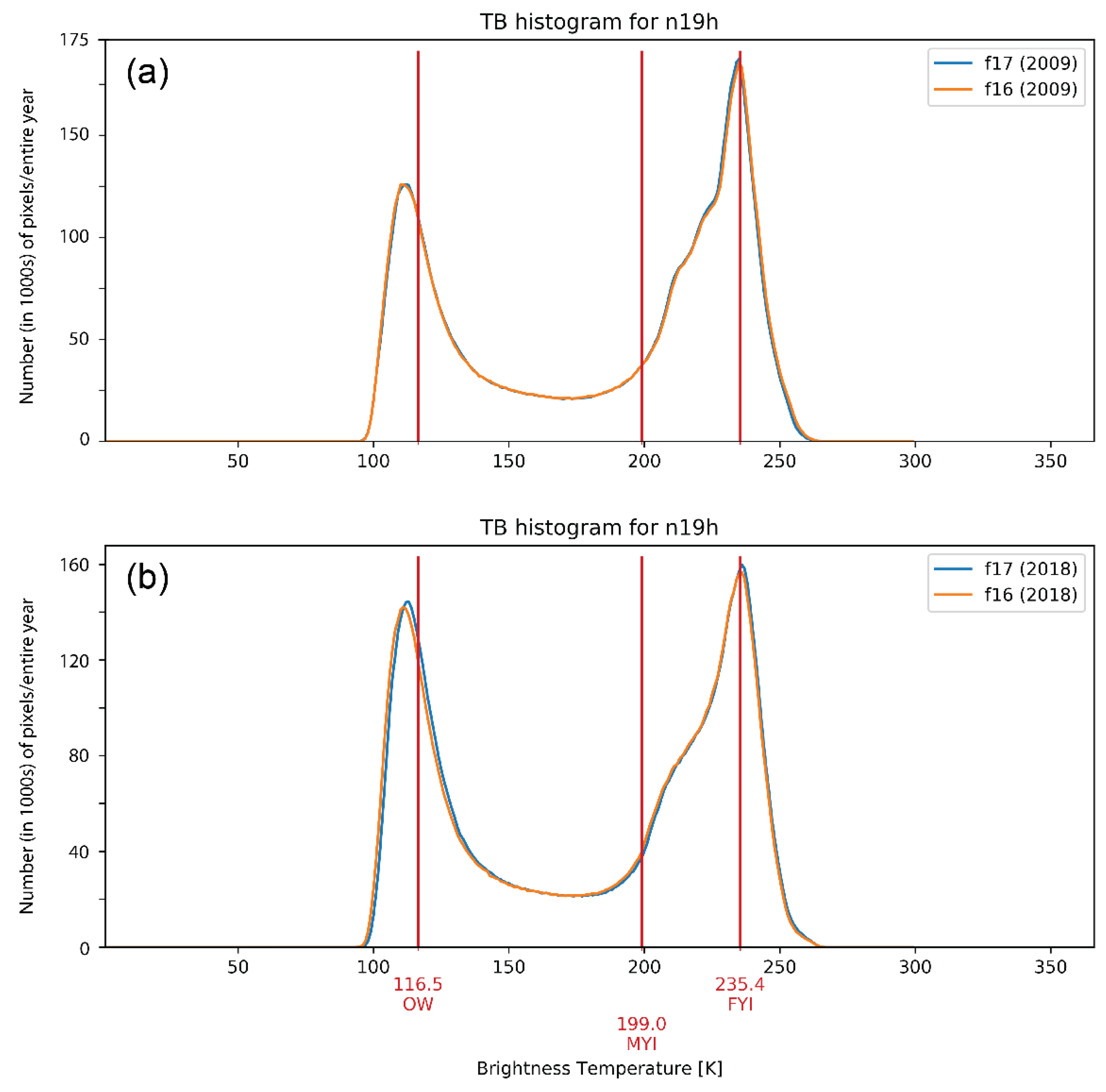
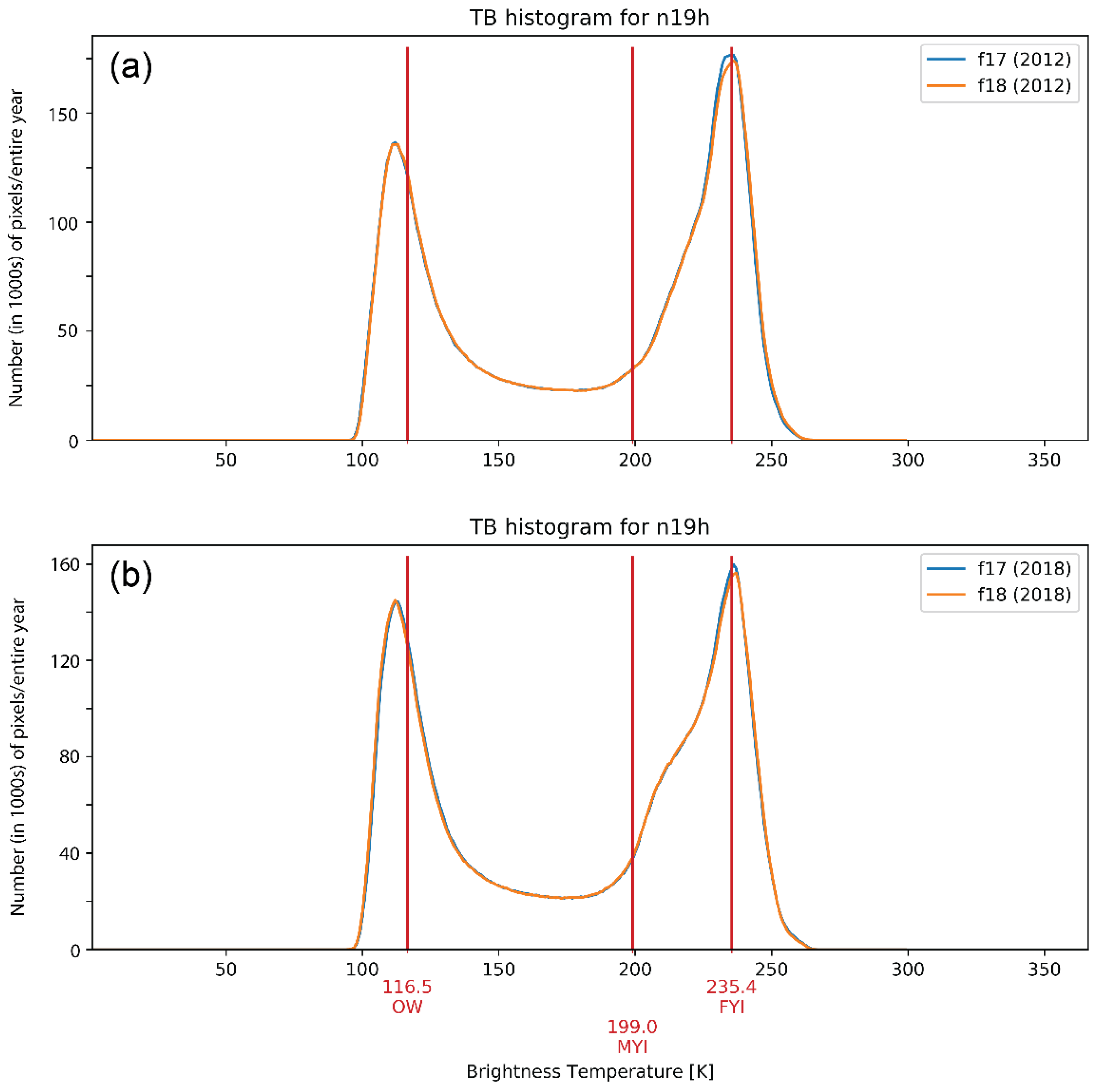
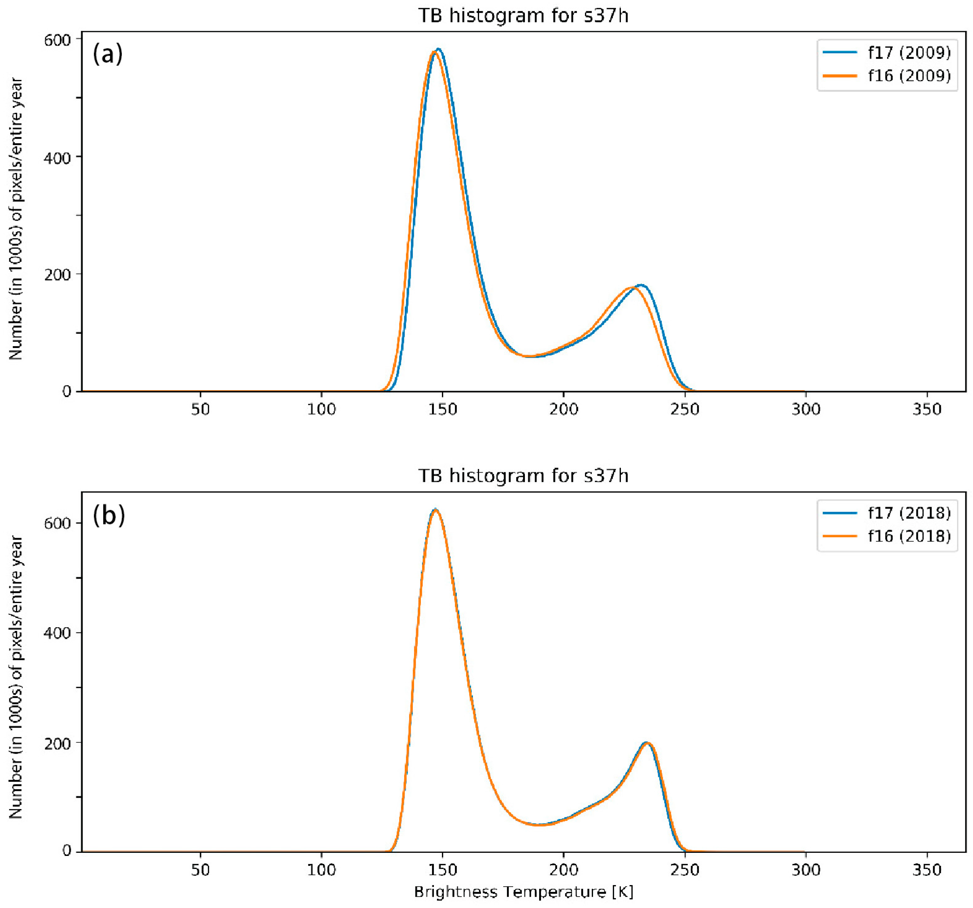
3.1. Comparison of Sensors in 2018

First, examining 2018, the TB histograms of the sensors qualitatively match very well (Figure 2 and Figure 3 for 19H; see Supplement, Figures S1–S8, for other channels). The two peaks of the distributions, corresponding to open water (low TB) and 100% ice (high TB corresponding to primarily FYI) almost completely overlap. The peaks either fall into the same 1 K bin or differ by only one bin. Qualitatively, the distributions between the sensors appear to have better agreement than was documented for F13 (SSMI) and F17 (SSMIS) [21].

Tie point values for F17 used in the NSIDC processing of CLASS TBs [6] are overlaid on the histogram distributions. Note that the tie point values for open water are not coincident with the peaks, but are shifted to slightly warmer TBs. This accounts for variability in the ocean surface. TB over open water can be increased due to higher emission from surface roughening of the ocean (due to winds) and atmospheric emission (water vapor and cloud liquid water) [20]. Placing the tie point value at a higher TB than the peak accounts for these influences and yields 0% ice even when there is some emissive “noise” in the open water signal. For ice, the FYI tie point closely coincides with the peak for 19H in the Northern Hemisphere. However, the distribution does include higher TBs. This distribution beyond the FYI tie point reflects variability in the sea ice properties. Surface roughness, salinity, and snow properties all affect the emission. In the Southern hemisphere, the peak is shifted slightly lower than the FYI tie point; this means that peak distribution is slightly less than 100%. This likely reflects a more dynamic ice cover with more leads and open water in the Antarctic, particularly near the northern ice edge where the ice can be rather diffuse. Thus, the distribution around each tie point reflects variability in the microwave emission due to surface and atmospheric effects. In practice, this means that some retrievals by the sea ice concentration algorithm will obtain ice concentrations below 0% and above 100%. Since these are non-physical, such values are truncated to 0% and 100%. However, truncated values do effectively contribute to overall variability in the retrievals and should be considered when estimating concentration uncertainty, e.g., [12].

3.2. Comparison of Sensors in Different Years

As noted above (Table 1), while the F17 orbit has remained relatively stable, both the F16 and F18 platforms have experienced substantial drift in their orbits. Particularly near the equinoxes, when diurnal effects in the polar regions are strongest, this is a potential concern in that it may impart an artificial trend to sea ice fields if the TB distributions substantially change. To assess this, we compared the F16 and F18 TB distributions with the F17 distribution in 2009, 2012, and 2018. The F16 orbit varies by ~4 h between 2009 and 2018; the F18 orbit varies by ~2.5 h between 2012 and 2018. In contrast, the F17 orbit varies by only ~1 h across all years.

The comparisons show little change in the relative distributions of F17 and F16 19H TBs between 2009 and 2018 (Figure 4) and for F17 and F18 between 2012 and 2018 (Figure 5). There are different TB distributions between years because of different ice conditions, but the differences between the sensors appear consistent, i.e., all sensors track the different ice conditions similarly. There is a slight change in the F16 open water peak in 2018, but otherwise the distributions line up well with F17. Other channels show similar characteristics (not shown). Since the F17 orbit changes little, this indicates that, at least qualitatively, the orbital changes in F16 and F18 do not substantially affect the gridded TB fields.

The lone exception to this pattern is the F16 37H channel in the Antarctic (Figure 6). There is a notable shift, particularly in the ice peak. Interestingly, F16 has moved into better agreement with F17 (and F18) more recently, very closely matching in 2018. Since the NASA team algorithm does not employ the 37H channel, this drift in F16 does not impact NT concentration retrievals, however it would be important for other algorithms (e.g., Bootstrap) that do use the 37H channel. As noted above, the good overall TB agreement between sensors despite the satellite orbit drift is at least partly explained by the daily composite drop-in-the-bucket gridding, which mutes effects of changes in observation time by temporally averaging several swaths. Statistical methods could be used to assess the differences and adjust tie points to match the distributions and optimize consistency of sea ice products between sensors and over time, but our focus in this paper is to simply illustrate the differences between the distributions.

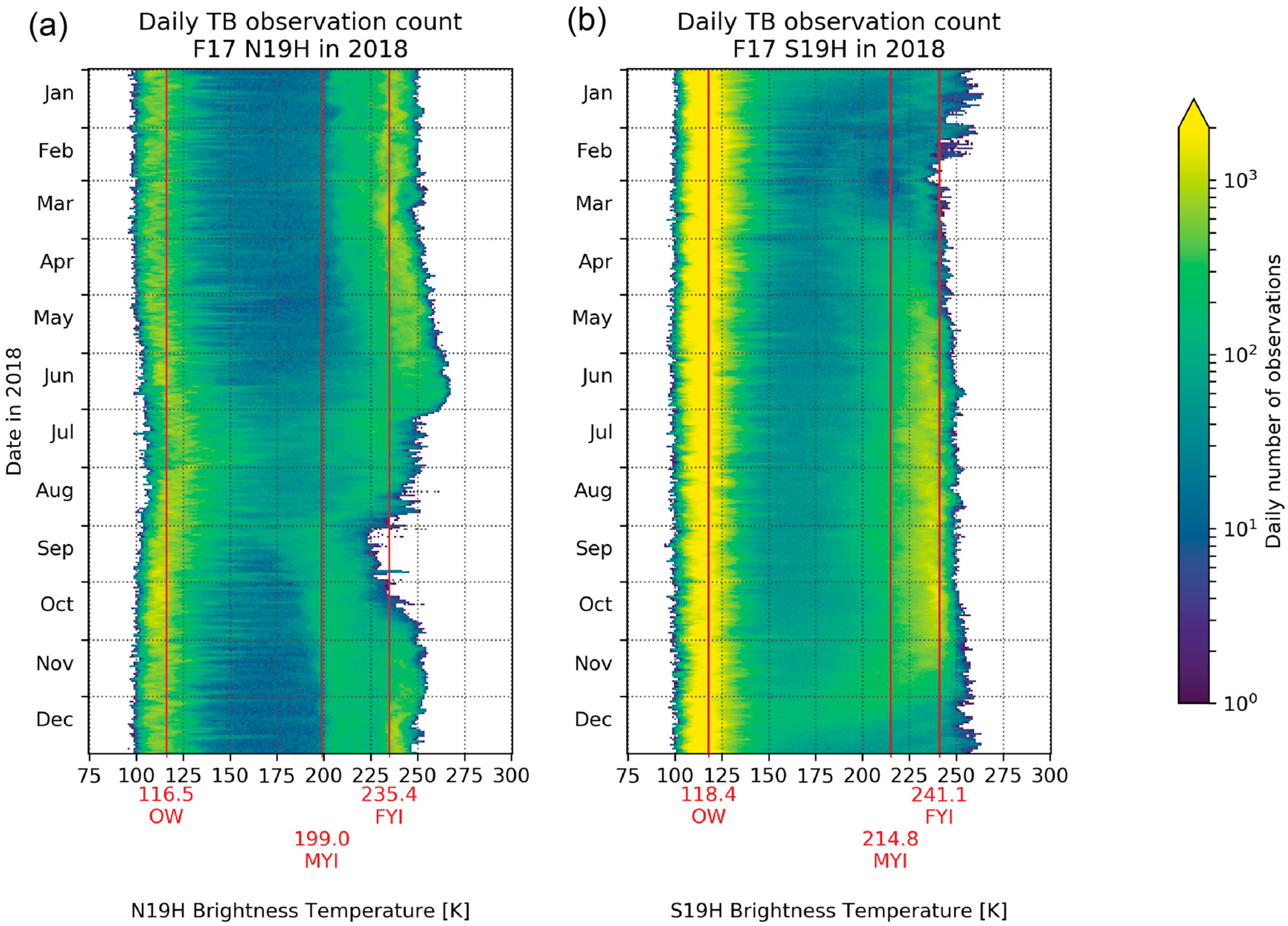
3.3. Daily Variations in Brightness Temperature Histograms

In the previous section, we showed that the annual average histograms of TBs qualitatively compare well between the F16, F17, and F18 SSMIS sensors, even across different years. Here, we investigate day-by-day variations in the histograms for each sensor, channel, and year. This also allows more precise quantification of the difference through analysis of the average values of the distribution peak.

It is clear that there is considerable daily and seasonal variation in the TB distribution (Figure 7). The open water (OW) peak is more consistent through the year, which is not surprising. TB is a function only of the emitting surface emissivity and the physical temperature. Water emissivity at these microwave frequencies is stable. The distribution around the water peak is due to the synoptic surface wind-surface roughening and atmospheric emission.

There is a slight increase in peak OW TB in the Arctic during June through August. This is likely an ocean surface temperature influence. As noted earlier, the Arctic domain used for the histograms is based on a monthly valid-ice mask encompassing all regions with sea ice plus a buffer of open water beyond based on a valid-ice climatology mask. With much lower summer sea ice extent in recent years, there is more open water and that water absorbs solar energy, warming the ocean surface.

The most notable characteristic in the distributions is the large variability in the ice peak, particularly during summer. There are two reasons for this. One is that FYI extent decreases through the summer and the MYI signature becomes more dominant. This is particularly prevalent in the Antarctic where nearly all of the seasonal ice cover is lost during the summer. Another factor, particularly in the Arctic, is the well-known surface melt and melt pond effect, e.g., [17]. At the microwave frequencies used by the NASA team algorithm (and most other algorithms), emission comes from the surface or very near the surface. Thus, liquid water on the ice surface contributes substantially to the retrieved microwave emission signature. This results in an underestimation of concentration.

To quantify these variations, the daily histogram distributions are averaged through each of the three years. In the Arctic, the full year is analyzed (

Table 2. Arctic annual average and standard deviation (SD) of daily brightness temperature histogram distribution water and ice peak values for F17 and differences between F16 and F18 with F17. The NASA Team F17 open water and FYI tie point (TP) values are also provided for reference.

Arctic		Annual Avg. Peak Value (K)			Annual Avg. SD Peak Value (K)
Year	Sensor	19V	19H	37V	19V	19H	37V
Water	OW TP	182.2	116.5	206.5
2009	F17	183.2	113.7	206.6	5.1	11.5	3.7
2012	F17	183.0	113.8	206.5	4.3	11.2	3.1
2018	F17	182.8	115.1	206.6	3.9	13.2	2.9
2009	F16-F17	–0.3	0.9	0.2	5.8	15.5	3.6
2012	F16-F17	–0.9	–0.3	0.1	3.6	15.2	3.2
2018	F16-F17	–0.2	–1.4	–0.3	4.8	17.8	2.1
2012	F18-F17	–1.1	0.1	0.0	5.0	14.6	2.5
2018	F18-F17	–0.8	–1.7	0.0	4.5	16.1	2.3
Ice	FYI TP	251.7	235.4	242.7
2009	F17	250.3	229.3	244.5	10.2	16.2	10.1
2012	F17	248.3	225.1	243.9	14.6	22.8	10.3
2018	F17	250.3	227.9	243.5	10.9	17.9	10.9
2009	F16-F17	0.1	–0.1	1.0	5.2	13.0	3.8
2012	F16-F17	0.1	0.3	0.4	5.7	17.1	3.2
2018	F16-F17	–0.7	–1.0	–0.6	6.1	11.6	4.2
2012	F18-F17	0.0	1.3	0.5	6.2	15.9	3.7
2018	F18-F17	–0.6	–0.1	–0.4	5.9	11.7	4.1

). In the Antarctic, the small amount of remaining summer ice leads to very high variability, so only the winter (May through October) period is analyzed here (

Table 3. Antarctic May–October average and standard deviation (SD) of daily brightness temperature histogram distribution water and ice peak values for F17 and differences between F16 and F18 with F17. The NASA Team F17 open water and FYI (Type A) tie point (TP) values are also provided for reference.

Antarctic		May–Oct. Avg. Peak Value (K)			May–Oct. Avg. SD Peak Value (K)
Year	Sensor	19V	19H	37V	19V	19H	37V
Water	OW TP	187.7	118.4	208.9
2009	F17	183.0	113.8	206.8	1.3	3.1	1.3
2012	F17	183.3	114.5	207.0	1.3	2.9	1.1
2018	F17	182.5	113.5	206.2	1.3	3.1	1.3
2009	F16-F17	–0.6	–0.4	0.0	1.1	2.2	1.0
2012	F16-F17	–0.4	–0.3	0.2	0.8	1.7	0.8
2018	F16-F17	0.2	0.2	–0.1	1.1	2.3	1.0
2012	F18-F17	–1.3	0.1	–0.5	1.1	2.3	1.0
2018	F18-F17	–0.8	0.0	0.2	1.1	2.3	0.9
Ice	FYI TP	256.2	241.1	246.6
2009	F17	254.8	232.2	247.8	2.0	6.1	3.5
2012	F17	254.7	234.3	249.8	3.3	5.3	3.1
2018	F17	253.9	234.0	249.5	3.3	7.0	2.7
2009	F16-F17	0.2	0.1	0.2	1.0	8.1	3.0
2012	F16-F17	0.3	–0.8	0.5	3.4	8.7	1.6
2018	F16-F17	0.5	0.4	0.6	4.4	9.3	2.8
2012	F18-F17	–0.8	–0.6	–0.3	4.4	8.5	2.5
2018	F18-F17	0.2	1.0	0.3	3.8	8.1	1.8

). The full year statistics for the Antarctic are provided in the Supplement (Table S1).

In the Arctic, the open water and ice peaks are generally consistent for F17 in the three years, with the peak TB values within 1–2 K. The variability (standard deviation) is higher for ice than for water. This reflects both the inherent greater variability of the ice cover (ice type, snow cover) and the variation during the year due to changes in the distribution of FYI and MYI and melt effects. The 19H channel has the largest TB variability, both for open water and ice.

The differences of the F16 and F18 SSMIS with F17 are generally 1 K or less, which are of similar magnitude as the differences seen in earlier inter-sensor comparisons, e.g., [6,19,21]. The average differences between sensors is small compared to the intra-annual variability and the variability in the TB peak differences is on the same scale as the TB peak variation for a single sensor (i.e., F17). This means that the day-to-day and seasonal variations in the TB histogram from a single sensor are as great or greater than the differences in the TB histogram between sensors.

In the Antarctic, even examining only winter conditions, the ice peak variability is higher than the water peak. Similarly, as for the Arctic, the variability from a single sensor is higher than the differences between sensors. These results again indicate that on a given day, uncertainty in TB values from any one sensor are as high or higher than the difference between TBs from different sensors. However, for long-term trends, even small average differences can result in biases in time series. Thus, the difference here should be examined further for potential tie point adjustments in long-term time series.

In terms of any effect of orbit drift, the results are not definitive. Some channels on F16 and F18 do show a small trend in the differences with F17. For example, for 19H in the Arctic, the F16-F17 difference changes from 0.9 K to –0.3 K to –1.4 K from 2009 to 2012 to 2018. However, other channels do not show any clear trend; for example, F16-F17 19V changes from –0.3 K to –0.9 K and then back to –0.2 K. If there is an effect from orbital drift, it appears small and not necessarily consistent.

3.4. Sensitivity of Sea Ice Concentration to Different Sensors

A final assessment of the impact of the different sensors and years is done by examining the effect of the brightness temperatures on NASA Team sea ice concentration estimates. Concentration maps between the different sensors show only small differences over most of the ice cover, with larger differences only near the ice edge (see Supplement, Figures S9 and S10). Here, we illustrate the differences by calculating the concentration corresponding to the TBs of the peaks of each channel’s histogram. Concentrations were calculated for each day and then annual averages and standard deviations were calculated (

Table 4. Annual average NT sea ice concentration (%) values corresponding to the daily TB histogram peak values for water and ice for F17 and the F16-F17 and F18-F17 difference. Standard deviation values are in parentheses.

		Arctic (%)		Antarctic (%)
Year	Sensor	Water	Ice*	Water	Ice*
2009	F17	–3.9 (4.4)	97.7 (6.6)	–4.3 (2.5)	80.1 (22.5)
2012	F17	–3.8 (4.3)	97.1 (3.7)	–4.0 (2.5)	84.6 (20.5)
2018	F17	–3.5 (4.0)	97.9 (6.2)	–4.2 (2.5)	78.1 (27.8)
2009	F16-F17	–0.3 (3.9)	0.3 (6.4)	–0.6 (2.0)	0.5 (10.1)
2012	F16-F17	–0.8 (3.1)	0.0 (2.3)	–0.7 (1.6)	–0.4 (11.8)
2018	F16-F17	–0.7 (3.1)	–0.4 (8.9)	–0.7 (2.1)	0.2 (11.5)
2012	F18-F17	–0.1 (3.5)	1.1 (2.5)	–0.1 (2.0)	–0.2 (16.2)
2018	F18-F17	–0.5 (2.9)	0.8 (5.9)	–0.6 (1.9)	0.7 (11.4)

*Ice values are for winter only (December–May for the Arctic; June–November for the Antarctic).

). As expected from the histogram distribution, the water peak is a negative concentration, which compensates for atmospheric effects. The ice peak corresponds fairly closely overall with the FYI tie point. However, in summer, due to melt and loss of FYI, the peak drops to a lower temperature. Thus, only the winter period (Dec–May in the Arctic; Jun–Nov in the Antarctic) are used in the calculations here. Full year statistics (not shown) are similar with the only significant difference being a lower average total concentration; differences between sensors and years are consistent with those shown here (Table 4). The winter ice peak TB values correspond to near 100% ice for the Arctic and 80–85% ice concentration for the Antarctic. This is consistent with the well-known low bias in NT concentrations in the Antarctic [27].

The differences between sensors is small in all years, <1% concentration with a standard deviation of <10% except for the ice peak in the Antarctic, which has values ~10–15%. However, in light of the overall variability in the Antarctic ice peak (20–30% standard deviation for F17), this variability is not surprising. This means that the TB differences between sensors appear to not substantially affect the total concentration. There is also not any obvious systematic change over the years, suggesting that any effect of sensor drift is small. We note that this sensitivity test is for only the water and ice peak TB values in the histogram, i.e., near 0% and near 100% sea ice conditions. It is possible that intermediate concentration values may show larger differences. Also, even small differences in concentration can potentially lead to biases in sea ice extent as grid cells with concentrations near the 15% threshold flip between “ice” and “ice-free”.

4. Discussion

The focus of this study is to assess the near-real-time TBs from NOAA CLASS that NSIDC distributes as daily composite polar stereographic grids and the potential impact of their differences on sea ice concentration estimates from the NASA team algorithm. NSIDC switched the NRT SSMIS sensor from F17 to F18 in 2016. Internal assessment at the time determined that TB agreement was reasonably good and the effects of the change on NRT sea ice concentration and extent fields from the NASA team algorithm were small. Thus, algorithm tie point adjustments were not necessary for near-real-time processing. This study confirms that any adjustments would be small and would not have a large effect on the concentration estimates. The effects of the impacts on sea ice extent estimates were assessed in [13] and differences were small and on the same scale as internal variability from a single sensor. Since 2016, the F17 SSMIS has largely been operating nominally. NSIDC is now considering making data from both F17 and F18 SSMIS, as well as F16 SSMIS, available.

Overall, there is good agreement between sensors with annual TB histograms matching very closely. There are small biases between sensors, but these are much smaller than intra- and inter-annual variations of TBs from a single sensor. The variation in the daily differences between sensors and is similar to the daily variation within a single sensor. Effectively, the variation in conditions of emissive properties of the surface are greater than the differences between sensors. This points to the potential advantage of using multiple sensors to provide an ensemble average TB estimate with accompanying uncertainty estimates. Similarly, the differences in concentration are small and are likely not critical for near-real-time processing.

While average biases between sensors are small, they are potentially important for production of long-term time series. The biases found here are similar in magnitude to those found in previous inter-sensor comparisons where tie point adjustments were made. Thus, when the long-term NASA team concentration product switches from its current F17 SSMIS source to F18, an inter-calibration and algorithm tie point adjustment would likely be beneficial to provide the most consistent long-term record. Such consistency is critical to assess trends, particularly where trend magnitudes are small, such as in the Antarctic.

One concern with the F16 and F18 SSMIS record is the substantial orbital drift of the satellites. This is particularly salient in terms of tie point adjustment. In the past, such adjustments occurred once during an overlap period. Some overlap periods were very short and possibly at non-optimal times of the year, which affects the quality of the adjustment [6]. However, even if a full-year of overlap is used to optimally adjust tie points for consistency, the orbit drift and changing observation times could erode that consistency over several years and introduce an artificial trend. The analysis here of potential sensor drift effects is not conclusive. The histogram comparisons between sensors do not show a systematic shift in all channels. Differences in average water and ice peak values show potential small trends in some channels. However, there isn’t an obvious systematic effect on the concentration estimates. Thus, the effect of sensor drift, if present, appears to be very small for concentration fields.

The high daily and intra-annual variability and the potential effect of orbital drift in the TB histogram distributions indicates that constant tie points have limitations. A recommendation here is to consider implementing dynamic (time-varying) tie points to the NASA team algorithm, as has been done for the Bootstrap and OSI-SAF products. Such an approach was investigated by [21] and showed promise, particularly for MYI concentration. Dynamic tie points automatically adjust for changes in sensor properties and orbital drift. They also adjust to changing surface conditions, such as surface melt. The onset of melt for Arctic sea ice is becoming earlier, e.g., [28]. With constant tie points, this trend in melt onset imparts a trend in concentration during the melt period.

Such enhancements would also benefit weather and climate forecasts at all temporal scales. An accurate surface boundary layer, especially in terms of ice vs. open ocean, is critical to obtaining accurate synoptic forecasts. For example, improvements in sea ice fields have increased the accuracy of polar ice and atmospheric circulation forecasts in U.S. Navy models [29,30]. While seasonal forecasts are less sensitive to initial conditions, an understanding of the stability of the microwave observed sea ice can inform the assessment of seasonal forecast models, which are becoming more relevant as the Arctic Ocean opens up to more human activity [31]. Finally, as noted earlier, uncertainties in the stability and consistency of sea ice extent records results in uncertainties in long-term climate trends, particularly when trends are small and/or borderline statistically significant [7].

5. Conclusions

Passive microwave brightness temperatures constitute a fundamental climate data record that is the foundation of several key geophysical parameters, with sea ice being one of the most iconic. The value of these TB records is their long-term, continuous record, their all sky capability over sea ice, and near-complete daily coverage. Compiling such a record requires stitching together data from a series of sensors and adjusting TBs to optimize consistency over time. Newer sensors, such as AMSR-E and AMSR2 provide enhanced capabilities and higher spatial resolution, but are not necessarily consistent with the longer-term SMMR-SSMI-SSMIS record.

Here, we have analyzed three SSMIS sensors, on the DMSP F16, F17, and F18 platforms, all currently (as of 1 July 2020) operating. Overall, there is good consistency between the sensor TBs, with histogram distributions nearly coincident. Differences in the histogram peak values for open water and sea ice are mostly within 1 K on average. The net effect of these TB differences corresponds to an average <1% NT concentration difference between sensors. The variability in the TB and concentration differences between sensors is nearly the same as the variability within a single sensor. Thus, for day-to-day quasi-operational sea ice concentration processing, such as those produced by the NSIDC DAAC, using any of the sensors is acceptable. The larger satellite orbit drift of the F16 and F18 platforms compared to F17 does not seem to have a large effect on the gridded daily-averaged TB fields. Some TB channels in F16 and F18 exhibit small trends relative to F17, which could be due to the orbital drift, but there is not a clear effect on concentration estimates.

Comparison of the three sensors suggests that all sensors provide useful information. Thus, providing data from all available sensors would be beneficial as more information is better than less information. Multiple observations can provide insight into the uncertainty range of a given (e.g., ensemble) TB estimate. Currently, the NSIDC DAAC does distribute another gridded TB product, on the EASE2 grid, which does include TB fields from all available SSMI and SSMIS sensors [32]. It could be beneficial to provide all sensors for the polar stereographic gridded fields as well.

Finally, the variability in the TB fields, both day-to-day, as well as seasonal and interannual, indicates that deriving static tie points for each sensor is not optimal. The NASA team algorithm concentration retrievals would benefit from implementing dynamic tie points, as has been done for the Bootstrap and OSI-SAF concentration products. This approach is currently being considered for a future reprocessing effort.

References

1. Perovich, D.; Meier, W.N.; Tschudi, M.; Farrell, S.; Hendricks, S.; Gerland, S.; Kaleschke, L.; Ricker, R.; Tian-Kunze, X.; Webster, M.; et al. Sea ice. In Arctic Report Card 2019; 2019. Available online: https://www.arctic.noaa.gov/Report-Card/Report-Card-2019 (accessed on 26 May 2020).
2. Parkinson, C.L. A 40-y record reveals gradual Antarctic sea ice increases followed by decreases at rates far exceeding the rates seen in the Arctic. Proc. Natl. Acad. Sci. USA 2019, 116, 14414–14423. [Google Scholar] [CrossRef] [PubMed] [Green Version]
3. Box, J.; Colgan, W.; Brown, R.; Wang, M.; Overland, J.; Walsh, J.; Bhatt, U.; Christensen, T.; Schmidt, N.; Lund, M.; et al. Key Indicators of Arctic Climate Change: 1971–2017. Environ. Res. Lett. 2019, 14, 045010. [Google Scholar] [CrossRef]
4. Meier, W.N.; Hovelsrud, G.; van Oort, B.; Key, J.; Kovacs, K.; Michel, C.; Granskog, M.; Gerland, S.; Perovich, D.; Makshtas, A.P.; et al. Arctic sea ice in transformation: A review of recent observed changes and impacts on biology and human activity. Rev. Geophys. 2014, 41. [Google Scholar] [CrossRef]
5. Comiso, J.C.; Nishio, F. Trends in the sea ice cover using enhanced and compatible AMSR-E, SSM/I, and SMMR data. J. Geophys. Res. 2008, 113, C02S07. [Google Scholar] [CrossRef]
6. Meier, W.N.; Khalsa, S.J.S.; Savoie, M.H. Intersensor calibration between F-13 SSM/I and F-17 SSMIS near-real-time sea ice estimates. IEEE Trans. Geosci. Remote Sens. 2011, 49, 3343–3349. [Google Scholar] [CrossRef]
7. Eisenman, I.; Meier, W.N.; Norris, J.R. A spurious jump in the satellite record: Has Antarctic sea ice expansion been overestimated? Cryosphere 2014, 8, 1289–1296. [Google Scholar] [CrossRef] [Green Version]
8. Cavalieri, D.J.; Parkinson, C.L.; Gloersen, P.; Zwally, H.J. Sea Ice Concentrations from Nimbus-7 SMMR and DMSP SSM/I-SSMIS Passive Microwave Data, Version 1; NASA National Snow and Ice Data Center Distributed Active Archive Center: Boulder, CO, USA, 1996. [Google Scholar] [CrossRef]
9. Comiso, J.C. Bootstrap Sea Ice Concentrations from Nimbus-7 SMMR and DMSP SSM/I-SSMIS, Version 3; NASA National Snow and Ice Data Center Distributed Active Archive Center: Boulder, CO, USA, 2017. [Google Scholar] [CrossRef]
10. Lavergne, T.; Sorensen, A.M.; Kern, S.; Tonboe, R.; Notz, D.; Aaboe, S.; Bell, L.; Dybkjær, G.; Eastwood, S.; Gabarro, C.; et al. Version 2 of the EUMETSAT OSI SAF and ESA CCI sea-ice concentration climate data records. Cryosphere 2019, 13, 49–78. [Google Scholar] [CrossRef] [Green Version]
11. Meier, W.N.; Fetterer, F.; Savoie, M.; Mallory, M.; Duerr, R.; Stroeve, J. NOAA/NSIDC Climate Data Record of Passive Microwave Sea Ice Concentration, Version 3; NSIDC, National Snow and Ice Data Center: Boulder, CO, USA, 2017. [Google Scholar] [CrossRef]
12. Kern, S.; Lavergne, T.; Notz, D.; Pedersen, L.T.; Tonboe, R.T.; Saldo, R.; Sørensen, A.M. Satellite passive microwave sea-ice concentration data set intercomparison: Closed ice and ship-based observations. Cryosphere 2019, 13, 3261–3307. [Google Scholar] [CrossRef] [Green Version]
13. Meier, W.N.; Stewart, J.S. Assessing uncertainties in sea ice extent climate indicators. Environ. Res. Lett. 2019, 14, 035005. [Google Scholar] [CrossRef]
14. Comiso, J.C.; Meier, W.N.; Gersten, R. Variability and trends in the Arctic sea ice cover: Results from different techniques. J. Geophys. Res. 2017, 122, 6883–6900. [Google Scholar] [CrossRef]
15. Fetterer, F.; Knowles, K.; Meier, W.N.; Savoie, M.; Windnagel, A.K. Sea Ice Index, Version 3; NSIDC, National Snow and Ice Data Center: Boulder, CO, USA, 2017. [Google Scholar] [CrossRef]
16. Ivanova, N.; Pedersen, L.T.; Tonboe, R.T.; Kern, S.; Heygster, G.; Lavergne, T.; Sørensen, A.; Saldo, R.; Dybkjær, G.; Brucker, L.; et al. Inter-comparison and evaluation of sea ice algorithms: Towards further identification of challenges and optimal approach using passive microwave observations. Cryosphere 2015, 9, 1797–1817. [Google Scholar] [CrossRef] [Green Version]
17. Kern, S.; Lavergne, T.; Notz, D.; Pedersen, L.T.; Tonboe, R.T. Satellite Passive Microwave Sea-Ice Concentration Data Set Intercomparison for Arctic Summer Conditions. Cryosphere Discuss. 2020. [Google Scholar] [CrossRef] [Green Version]
18. Cavalieri, D.J.; Gloersen, P.; Campbell, W.J. Determination of sea ice parameters with the NIMBUS 7 SMMR. J. Geophys. Res. 1984, 89, 5355–5369. [Google Scholar] [CrossRef]
19. Cavalieri, D.J.; Parkinson, C.L.; Gloersen, P.; Comiso, J.C.; Zwally, H.J. Deriving long-term time series of sea ice cover from satellite passive-microwave multisensor data sets. J. Geophys. Res. 1999, 104, 15803–15814. [Google Scholar] [CrossRef]
20. Maslanik, J.A. Effects of weather on the retrieval of sea ice concentration and ice type from passive microwave data. Int. J. Remote Sens. 1992, 13, 37–54. [Google Scholar] [CrossRef]
21. Cavalieri, D.J.; Parkinson, C.L.; DiGirolamo, N.; Ivanoff, A. Intersensor Calibration Between F13 SSMI and F17 SSMIS for Global Sea Ice Data Records. IEEE Geosci. Remote Sens. Lett. 2012, 9, 233–236. [Google Scholar] [CrossRef] [Green Version]
22. Ye, Y.; Heygster, G. Arctic multiyear concentration retrieval from SSM/I data using the NASA Team algorithm with dynamic tie points. In Towards an Interdisciplinary Approach in Earth System Science; Lohmann, G., Meggers, H., Unnithan, V., Wolf-Gladrow, D., Notholt, J., Bracher, A., Eds.; Springer Earth System Sciences; Springer: Cham, Switzerland, 2015; pp. 99–108. [Google Scholar] [CrossRef]
23. Maslanik, J.; Stroeve, J. Near-Real-Time DMSP SSMIS Daily Polar Gridded Sea Ice Concentrations, Version 1; NASA National Snow and Ice Data Center Distributed Active Archive Center: Boulder, CO, USA, 1999. [Google Scholar] [CrossRef]
24. Maslanik, J.; Stroeve, J. Near-Real-Time DMSP SSM/I-SSMIS Daily Polar Gridded Brightness Temperatures, Version 1; NASA National Snow and Ice Data Center Distributed Active Archive Center: Boulder, CO, USA, 1999. [Google Scholar] [CrossRef]
25. Meier, W.N.; Wilcox, H.; Hardman, M.A.; Stewart, J.S. DMSP SSM/I-SSMIS Daily Polar Gridded Brightness Temperatures, Version 5; NASA National Snow and Ice Data Center Distributed Active Archive Center: Boulder, CO, USA, 2019. [Google Scholar] [CrossRef]
26. Meier, W.N.; Stroeve, J.; Fetterer, F.; Savoie, M.; Wilcox, H. Polar Stereographic Valid Ice Masks Derived from National Ice Center Monthly Sea Ice Climatologies, Version 1; NASA National Snow and Ice Data Center Distributed Active Archive Center: Boulder, CO, USA, 2015. [Google Scholar] [CrossRef]
27. Comiso, J.C.; Cavalieri, D.J.; Parkinson, C.L.; Gloersen, P. Passive microwave algorithms for sea ice concentration: A comparison of two techniques. Remote Sens. Environ. 1997, 60, 357–384. [Google Scholar] [CrossRef]
28. Bliss, A.C.; Miller, J.A.; Meier, W.N. Comparison of passive microwave-derived early melt onset records on Arctic sea ice. Remote Sens. 2017, 9, 199. [Google Scholar] [CrossRef] [Green Version]
29. Hebert, D.A.; Allard, R.A.; Metzger, E.J.; Posey, P.G.; Preller, R.H.; Wallcraft, A.J.; Phelps, M.W.; Smedstad, O.M. Short-term sea ice forecasting: An assessment of ice concentration and ice drift forecasts using the U.S. Navy’s Arctic Cap Nowcast/Forecast System. J. Geophys. Res. 2015, 120, 8327–8345. [Google Scholar] [CrossRef] [Green Version]
30. Posey, P.G.; Metzger, E.J.; Wallcraft, A.J.; Hebert, D.A.; Allard, R.A.; Smedstad, O.M.; Phelps, M.W.; Fetterer, F.; Stewart, J.S.; Meier, W.N.; et al. Improving Arctic sea ice edge forecasts by assimilating high horizontal resolution sea ice concentration data into the US Navy’s ice forecast systems. Cryosphere 2015, 9, 1735–1745. [Google Scholar] [CrossRef] [Green Version]
31. Stroeve, J.; Hamilton, L.C.; Bitz, C.M. Blanchard-Wrigglesworth, E. Predicting September sea ice: Ensemble skill of the SEARCH Sea Ice Outlook 2008–2013. Geophys. Res. Lett. 2014, 41. [Google Scholar] [CrossRef] [Green Version]
32. Brodzik, M.J.; Long, D.G.; Hardman, M.A.; Paget, A.; Armstrong, R. MEaSUREs Calibrated Enhanced-Resolution Passive Microwave Daily EASE-Grid 2.0 Brightness Temperature ESDR, Version 1; NASA National Snow and Ice Data Center Distributed Active Archive Center: Boulder, CO, USA, 2020. [Google Scholar] [CrossRef]
Figure 1. Example of PR and GR values from F17 SSMIS for 28 February 2018. The triangle pattern is outlined in red with the 100% surface types noted and other concentration percentages sketched in. Water values are colored in blue and he GR weather filter threshold line is in light blue.
Remotesensing 12 02197 g001
Figure 2. Annual histogram of Arctic (Northern Hemisphere) 19H TBs for 2018 for SSMIS on (a) F17 and F16, and (b) F17 and F18. The F17 tie point values for open water (OW), FYI, and MYI are overlaid in red.
Remotesensing 12 02197 g002
Figure 3. Annual histogram of Antarctic (Southern Hemisphere) 19H TBs for 2018 for SSMIS on (a) F17 and F16, and (b) F17 and F18. The F17 tie point values for open water (OW), FYI, and MYI are overlaid in red.
Remotesensing 12 02197 g003
Figure 4. Annual histogram of Arctic (Northern Hemisphere) 19H TBs for F17 and F16 SSMIS in (a) 2009, and (b) 2018 (same as in Figure 2a). The F17 tie point values for open water (OW), FYI, and MYI are overlaid in red.
Remotesensing 12 02197 g004
Figure 5. Annual histogram of Arctic (Northern Hemisphere) 19H TBs for F17 and F18 SSMIS in (a) 2009, and (b) 2018 (same as in Figure 2b). The F17 tie point values for open water (OW), FYI, and MYI are overlaid in red.
Remotesensing 12 02197 g005
Figure 6. Annual histogram of Antarctic (Southern Hemisphere) 37H TBs for F17 and F16 SSMIS in (a) 2009, and (b) 2018. Note that 37H is not used in the NT algorithm.
Remotesensing 12 02197 g006
Figure 7. Daily histogram 19H TBs for F17 and F16 SSMIS for (a) Arctic (Northern Hemisphere), and (b) Antarctic (Southern Hemisphere). The x-axis is TB (K) with F17 tie points overlaid in red. The y-axis is time, starting with 1 January at the top, ending with 31 December at the bottom. The color scale is the number of observations in each 1 K bin for each day.
Remotesensing 12 02197 g007