Classification of Sea Ice Types in Sentinel-1 SAR Data Using Convolutional Neural Networks


Abstract
:
1. Introduction
2. Data and Preprocessing
2.1. Satellite Data
2.2. Expert Data
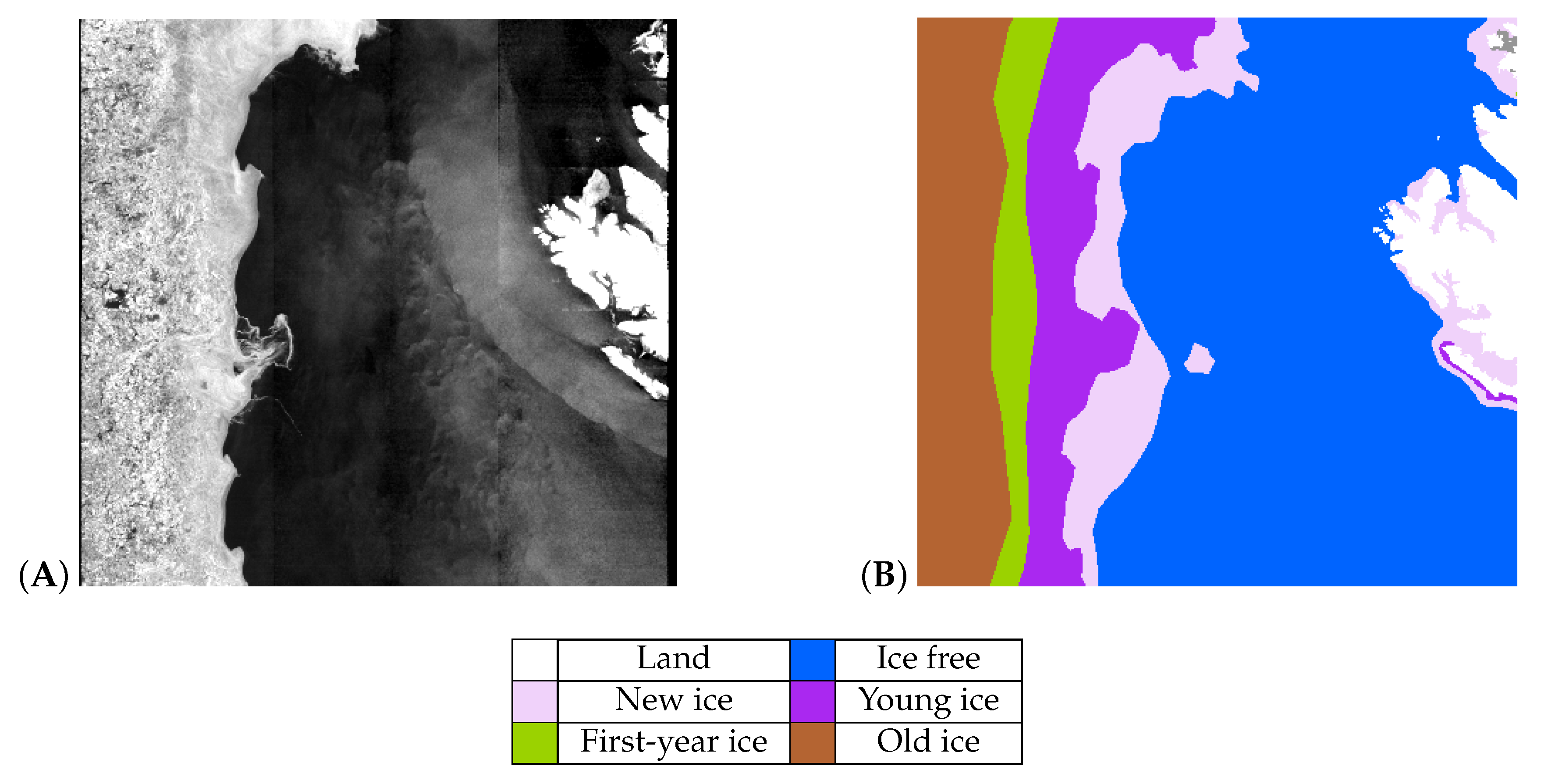
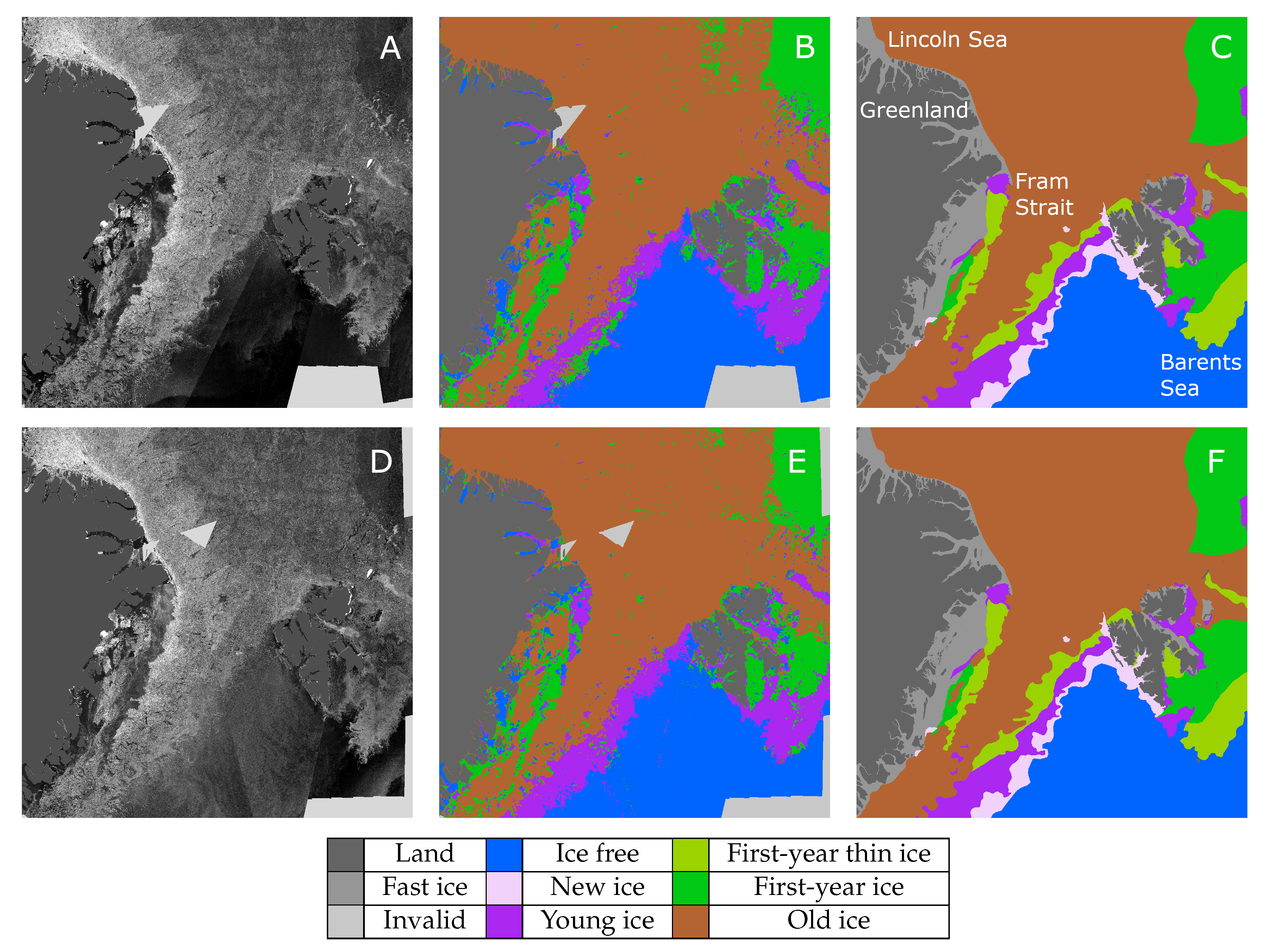
- Ice free (water) (WMO codes: 1)
- Young ice (WMO codes: 83–85)
- First-year ice (WMO codes: 87–94)
- Old ice (WMO codes: 95–97)
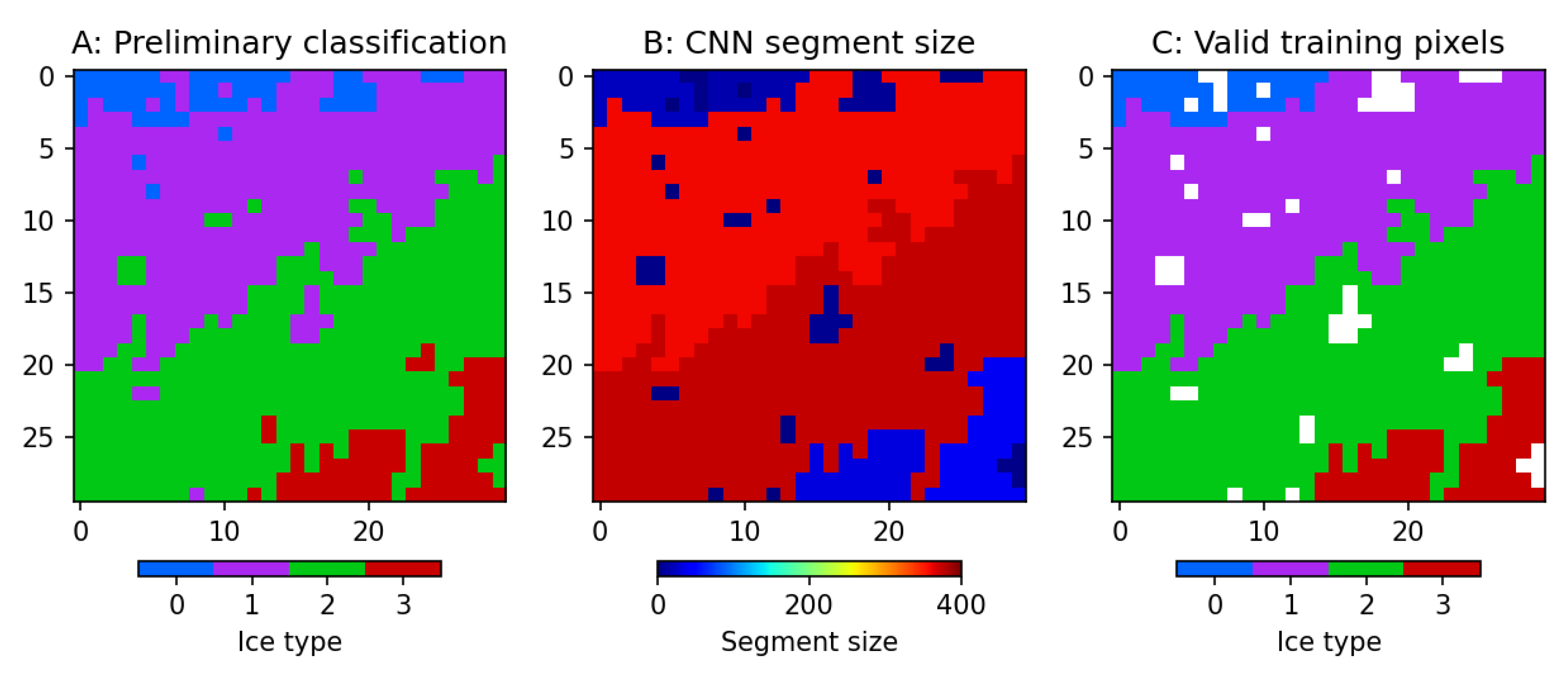
2.3. Preparation of a Combined Dataset
3. CNN Architecture and Training
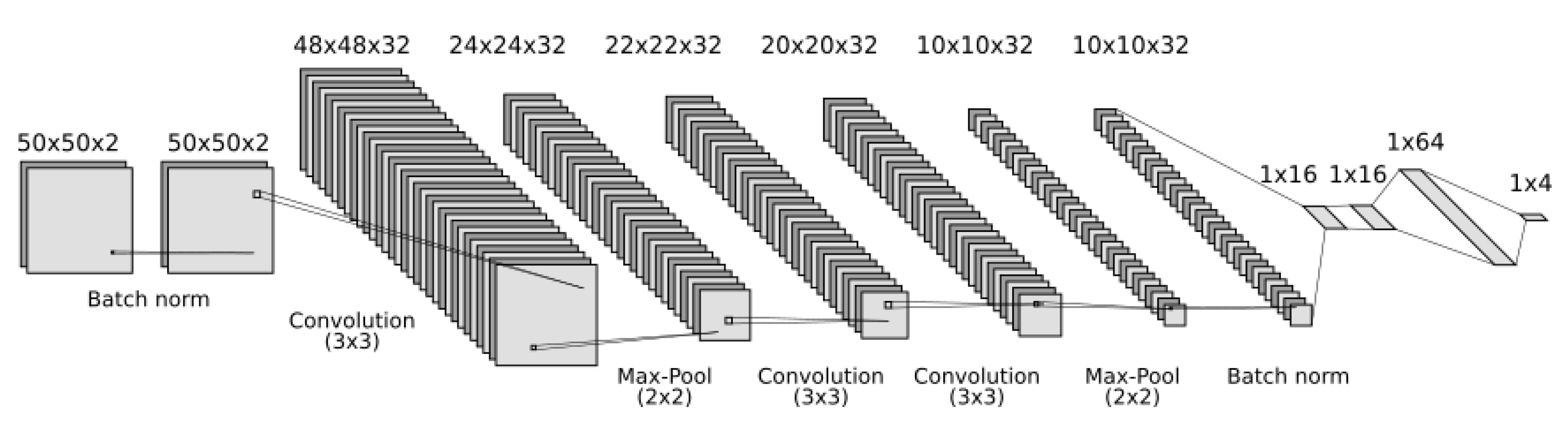
3.1. CNN Architecture
3.2. CNN Training
3.3. Validation Metrics
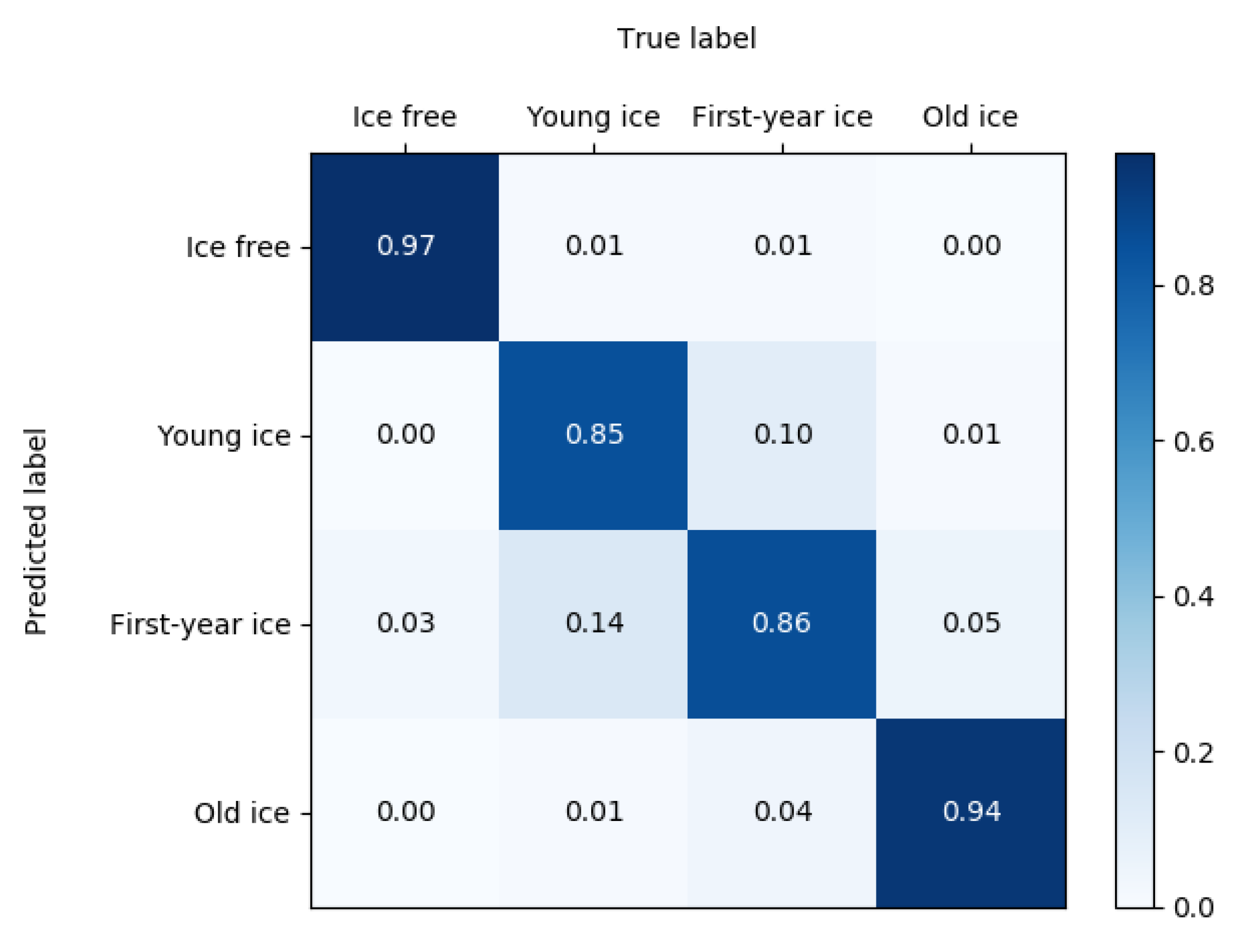
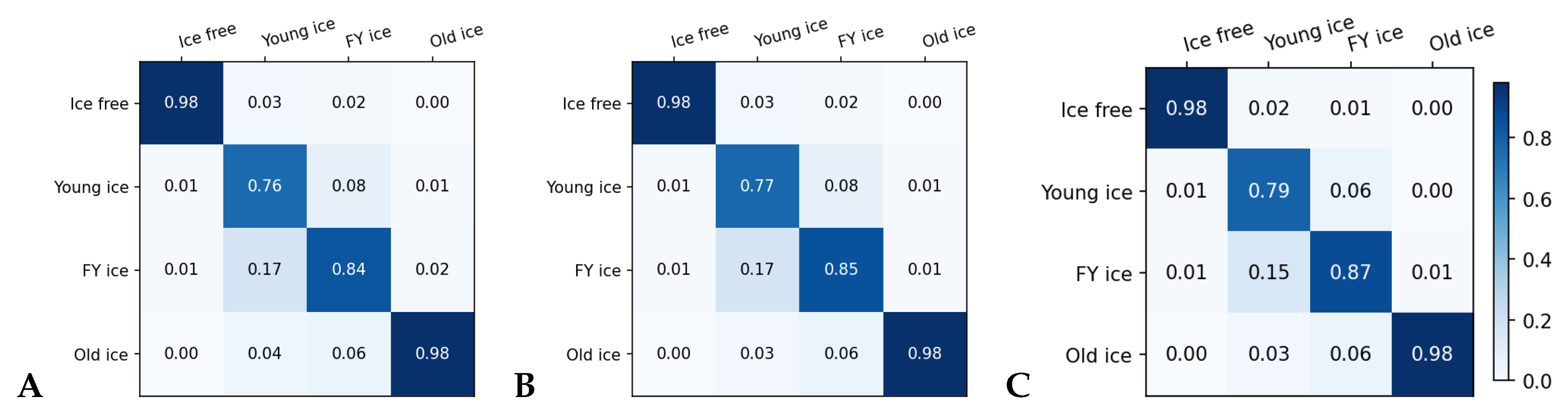
- The confusion matrix: An element of the matrix at the row r and column c is the number of samples predicted in the class r over the number of samples in the class c. A perfect classification would lead to a diagonal confusion matrix with 1 on the diagonal and 0 elsewhere. Each column sums up to 1.
- The accuracy per class (diagonal of confusion matrix) is the ratio of the correctly predicted samples of a given class over the total number of samples of the same class.
- The overall accuracy is the ratio of the correctly predicted samples over all the samples in the validation set. Overall accuracy is average accuracy per class weighted by class size.
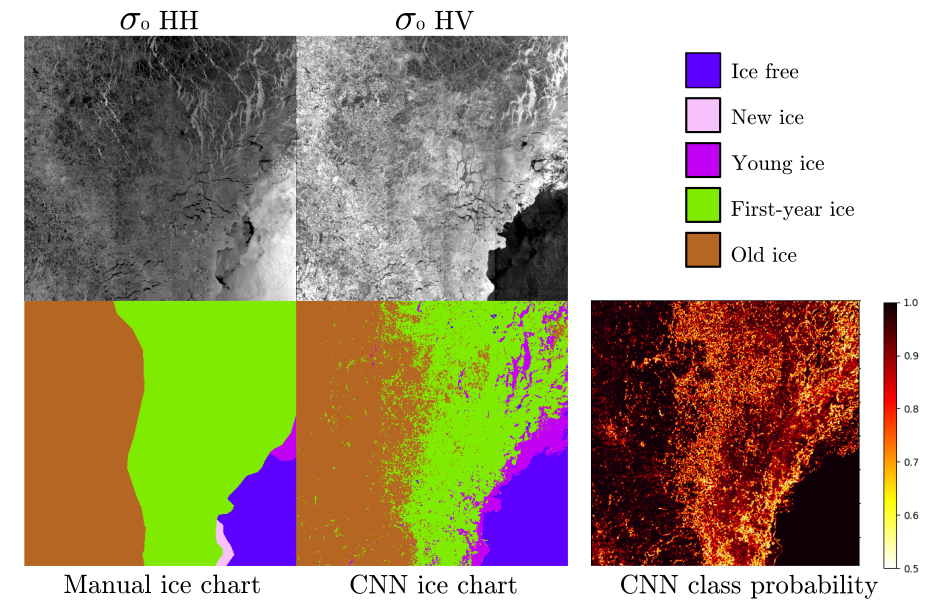
4. Results
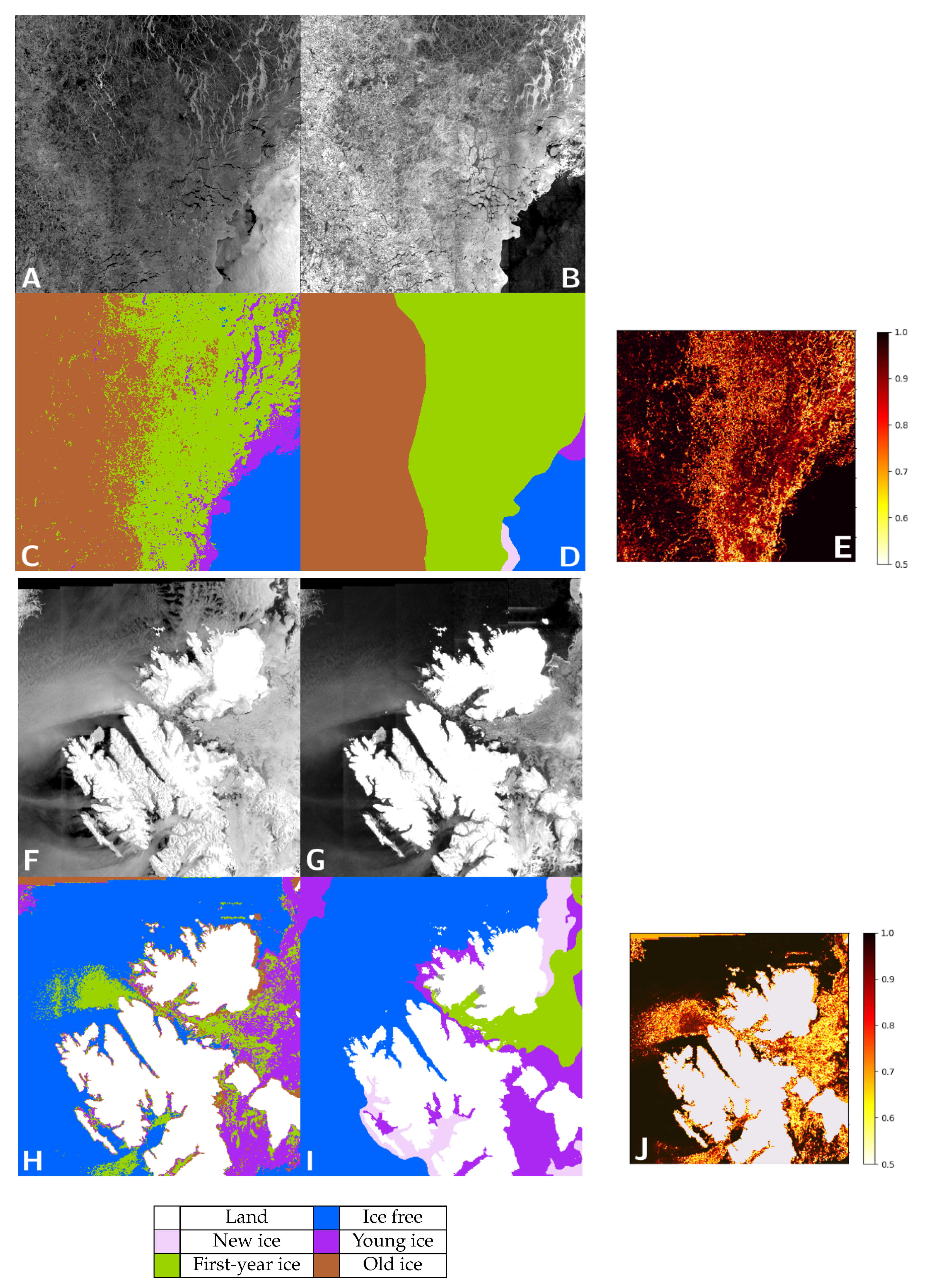
4.1. CNN-2018
4.2. CNN-2020
5. Sensitivity Study
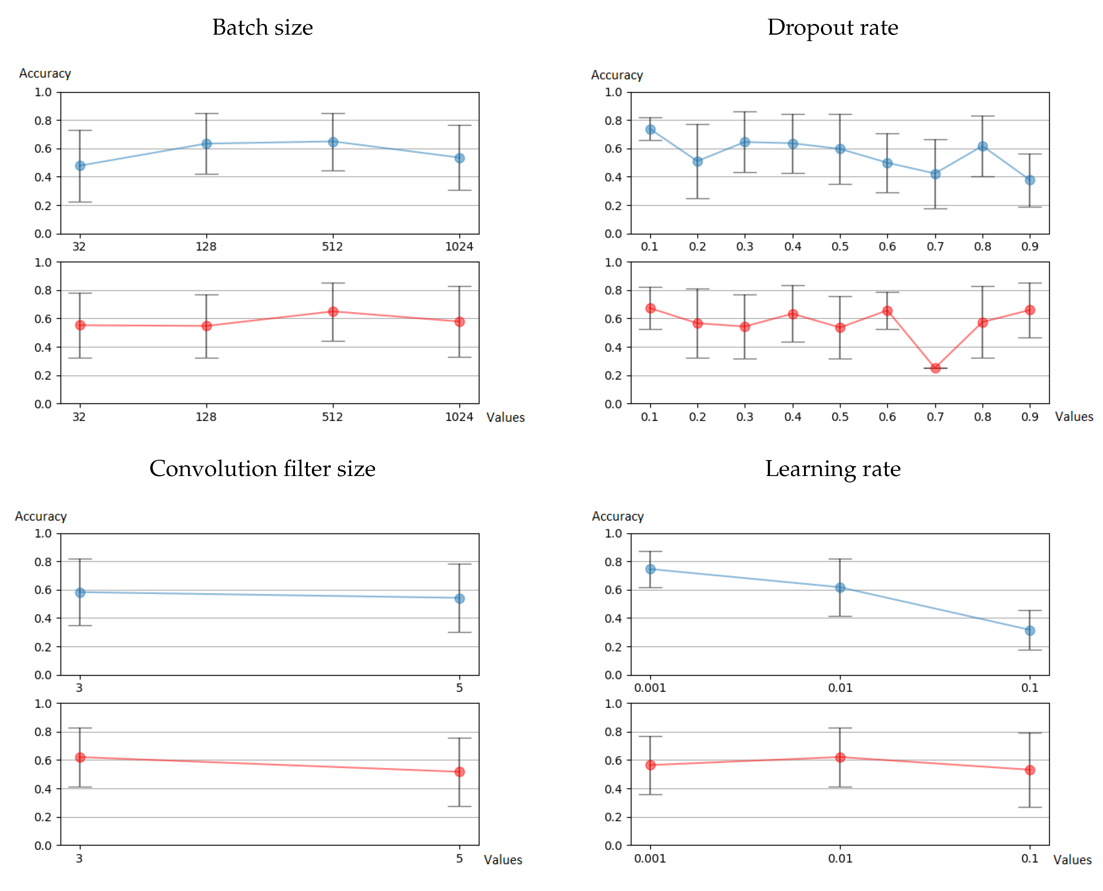
5.1. CNN Hyperparameter Sensitivity
| Algorithm 1: Randomized search algorithm for hyperparameters. |
 |
5.2. Sensitivity to Preprocessing Parameters
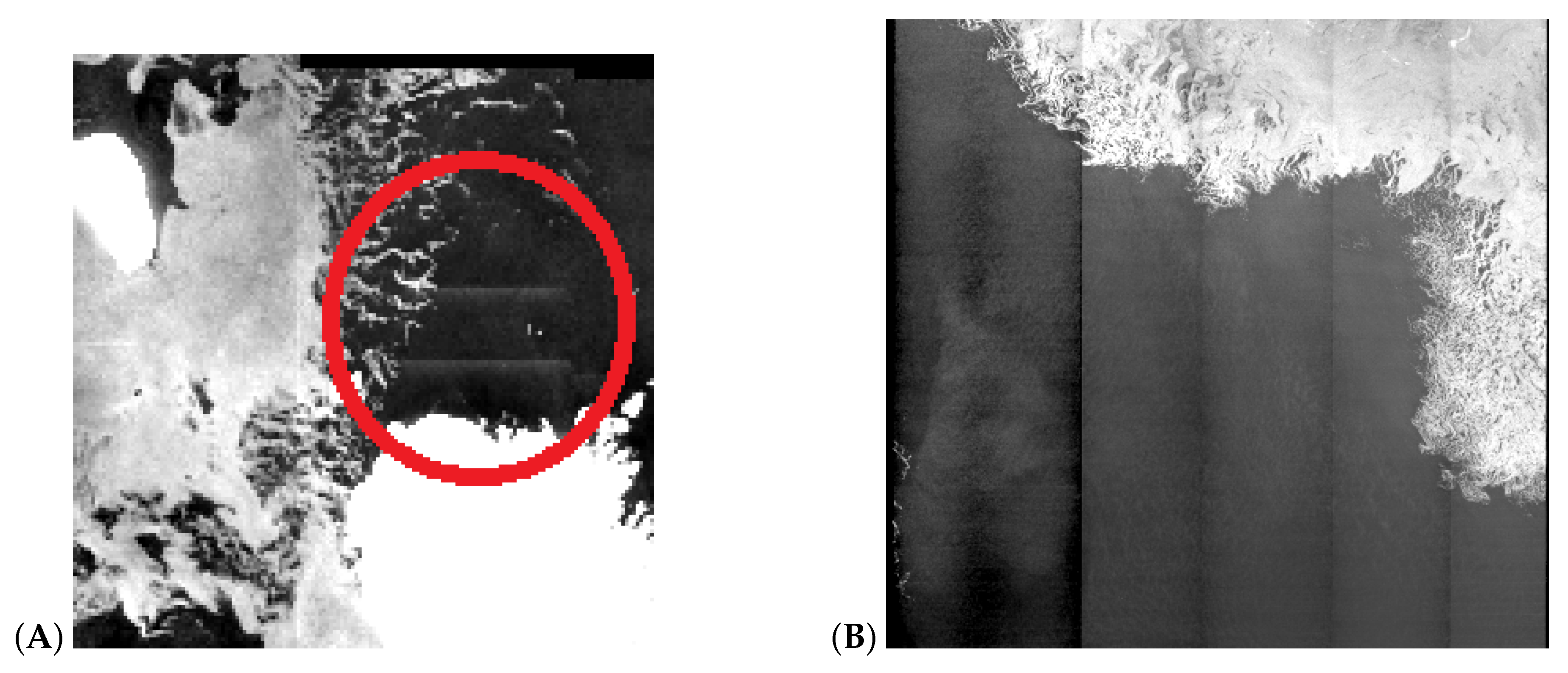
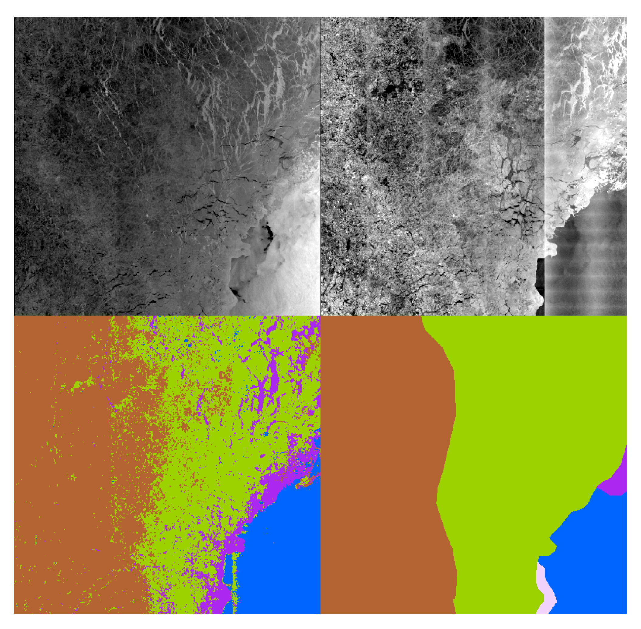
5.3. Impact of Thermal Noise and other Properties of Input Data
6. Discussion
7. Conclusions
Author Contributions
Funding
Acknowledgments
Conflicts of Interest
References
- Joint WMO-IOC Technical Commission for Oceanography and Marine Meteorology. Ice Chart Colour Code Standard; Version 1.0; World Meteorological Organization & Intergovernmental Oceanographic Commission: Geneva, Switzerland, 2014. [Google Scholar]
- Sentinel-1 SAR, ESA. Available online: https://sentinel.esa.int/web/sentinel/user-guides/sentinel-1-sar (accessed on 4 June 2020).
- Jackson, C.R.; Apel, J.R. Synthetic Aperture Radar Marine User’s Manual; Jackson, C.R., Apel, J.R., Eds.; National Oceanic and Atmospheric Administration: Washington DC, USA, 2004.
- Leigh, S.; Wang, Z.; Clausi, D.A. Automated Ice–Water Classification Using Dual Polarization SAR Satellite Imagery. IEEE Trans. Geosci. Remote Sens. 2014, 52, 5529–5539. [Google Scholar] [CrossRef]
- Fors, A.S.; Brekke, C.; Doulgeris, A.P.; Eltoft, T.; Renner, A.H.H.; Gerland, S. Late-summer sea ice segmentation with multi-polarisation SAR features in C and X band. Cryosphere 2016, 10, 401–415. [Google Scholar] [CrossRef] [Green Version]
- Zakhvatkina, N.; Korosov, A.; Muckenhuber, S.; Sandven, S.; Babiker, M. Operational algorithm for ice–water classification on dual-polarized RADARSAT-2 images. Cryosphere 2017, 11, 33–46. [Google Scholar] [CrossRef] [Green Version]
- Zakhvatkina, N.; Smirnov, V.; Bychkova, I. Satellite SAR Data-based Sea Ice Classification: An Overview. Geosciences 2019, 9, 152. [Google Scholar] [CrossRef] [Green Version]
- Komarov, A.S.; Buehner, M. Improved Retrieval of Ice and Open Water From Sequential RADARSAT-2 Images. IEEE Trans. Geosci. Remote Sens. 2019, 57, 3694–3702. [Google Scholar] [CrossRef]
- Aldenhoff, W.; Heuzé, C.; Eriksson, L.E. Comparison of ice/water classification in Fram Strait from C- and L-band SAR imagery. Ann. Glaciol. 2018, 59, 112–123. [Google Scholar] [CrossRef] [Green Version]
- Aldenhoff, W.; Eriksson, L.E.B.; Ye, Y.; Heuzé, C. First-Year and Multiyear Sea Ice Incidence Angle Normalization of Dual-Polarized Sentinel-1 SAR Images in the Beaufort Sea. IEEE J. Sel. Top. Appl. Earth Obs. Remote Sens. 2020, 13, 1540–1550. [Google Scholar] [CrossRef]
- Karvonen, J. A sea ice concentration estimation algorithm utilizing radiometer and SAR data. Cryosphere 2014, 8, 1639–1650. [Google Scholar] [CrossRef] [Green Version]
- Karvonen, J. Baltic Sea Ice Concentration Estimation Using SENTINEL-1 SAR and AMSR2 Microwave Radiometer Data. IEEE Trans. Geosci. Remote Sens. 2017, 55, 2871–2883. [Google Scholar] [CrossRef]
- Komarov, A.S.; Buehner, M. Detection of First-Year and Multi-Year Sea Ice from Dual-Polarization SAR Images Under Cold Conditions. IEEE Trans. Geosci. Remote Sens. 2019, 57, 9109–9123. [Google Scholar] [CrossRef]
- Lohse, J.; Doulgeris, A.P.; Dierking, W. An Optimal Decision-Tree Design Strategy and Its Application to Sea Ice Classification from SAR Imagery. Remote Sens. 2019, 11, 1574. [Google Scholar] [CrossRef] [Green Version]
- Park, J.W.; Korosov, A.A.; Babiker, M.; Won, J.S.; Hansen, M.W.; Kim, H.C. Classification of Sea Ice Types in Sentinel-1 SAR images. Cryosphere Discuss. 2019, 2019, 1–23. [Google Scholar] [CrossRef] [Green Version]
- Park, J.W.; Korosov, A.A.; Babiker, M.; Sandven, S.; Won, J.S. Efficient Thermal Noise Removal for Sentinel-1 TOPSAR Cross-Polarization Channel. IEEE Trans. Geosci. Remote Sens. 2017, 56, 1555–1565. [Google Scholar] [CrossRef]
- Park, J.W.; Won, J.S.; Korosov, A.; Babiker, M.; Miranda, N. Textural Noise Correction for Sentinel-1 TOPSAR Cross-Polarization Channel Images. IEEE Trans. Geosci. Remote Sens. 2019, 57, 4040–4049. [Google Scholar] [CrossRef]
- Wang, L.; Scott, K.A.; Clausi, D.A. Sea Ice Concentration Estimation during Freeze-Up from SAR Imagery Using a Convolutional Neural Network. Remote Sens. 2017, 9, 408. [Google Scholar] [CrossRef]
- Malmgren-Hansen, D.; Nielsen, A.A.; Kreiner, M.B.; Saldo, R.; Skriver, H.; Toudal Pedersen, L.; Lavelle, J.; Buus-Hinkler, J. High-Resolution Sea Ice Maps with Convolutional Neural Networks. In Proceedings of the 2019 ESA Living Planet Symposium, LPS 2019, Milan, Italy, 13–17 May 2019. [Google Scholar]
- Seger, C. An Investigation of Categorical Variable Encoding Techniques in Machine Learning: Binary Versus One-Hot and Feature Hashing; Technical Report 2018:596; KTH, School of Electrical Engineering and Computer Science (EECS): Stockholm, Sweden, 2018. [Google Scholar]
- Glorot, X.; Bordes, A.; Bengio, Y. Deep sparse rectifier neural networks. In Proceedings of the Fourteenth International Conference on Artificial Intelligence and Statistics, Ft. Lauderdale, FL, USA, 11–13 April 2011; pp. 315–323. [Google Scholar]
- Ioffe, S.; Szegedy, C. Batch normalization: Accelerating deep network training by reducing internal covariate shift. arXiv 2015, arXiv:1502.03167. [Google Scholar]
- Krizhevsky, A.; Sutskever, I.; Hinton, G.E. Imagenet classification with deep convolutional neural networks. In Proceedings of the Advances in Neural Information Processing Systems, Lake Tahoe, NV, USA, 3–6 December 2012; pp. 1097–1105. [Google Scholar]
- Srivastava, N.; Hinton, G.; Krizhevsky, A.; Sutskever, I.; Salakhutdinov, R. Dropout: A simple way to prevent neural networks from overfitting. J. Mach. Learn. Res. 2014, 15, 1929–1958. [Google Scholar]
- Kingma, D.P.; Ba, J. Adam: A Method for Stochastic Optimization. arXiv 2014, arXiv:cs.LG/1412.6980. [Google Scholar]
- Korosov, A.; Boulze, H. s1_icetype_cnn. 2020. Available online: https://doi.org/10.5281/zenodo.3828992 (accessed on 4 June 2020).
- Korosov, A.; Hansen, M.W.; Dagestad, K.F.; Yamakawa, A.; Vines, A. Nansat: A Scientist-Orientated Python Package for Geospatial Data Processing. J. Open Res. Softw. 2016, 4, e39. [Google Scholar] [CrossRef] [Green Version]
- European Centre for Medium-Range Weather Forecasts. 2020. Available online: https://www.ecmwf.int/en/forecasts (accessed on 4 June 2020).
- Bergstra, J.; Bengio, Y. Random Search for Hyper-parameter Optimization. J. Mach. Learn. Res. 2012, 13, 281–305. [Google Scholar]
- Tsai, Y.L.S.; Dietz, A.; Oppelt, N.; Kuenzer, C. Wet and Dry Snow Detection Using Sentinel-1 SAR Data for Mountainous Areas with a Machine Learning Technique. Remote Sens. 2019, 11, 895. [Google Scholar] [CrossRef] [Green Version]
- Jensen, O. The International Code for Ships Operating in Polar Waters: Finalization, Adoption and Law of the Sea Implications. Arct. Rev. 2016, 7, 60–82. [Google Scholar] [CrossRef] [Green Version]
- Sakov, P.; Evensen, G.; Bertino, L. Asynchronous data assimilation with the EnKF. Tellus A 2010, 62, 24–29. [Google Scholar] [CrossRef] [Green Version]
- Sensoy, M.; Kaplan, L.; Kandemir, M. Evidential deep learning to quantify classification uncertainty. In Proceedings of the Advances in Neural Information Processing Systems, Montréal, QC, Canada, 3–8 December 2018; pp. 3179–3189. [Google Scholar]
- Gal, Y.; Ghahramani, Z. Dropout as a bayesian approximation: Representing model uncertainty in deep learning. In Proceedings of the International Conference on Machine Learning, New York, NY, USA, 19–24 June 2016; pp. 1050–1059. [Google Scholar]


| Learning Rate | Dropout Rate | Batch Size n | L2 Regularization Parameter |
|---|---|---|---|
| 0.001 | 0.1 | 512 | 0.001 |
| CNN Name | OS | CPU | RAM, GB | GPU |
|---|---|---|---|---|
| CNN-2018 | Windows 10 | Intel Core i7-7500U 2 × 2.7 GHz | 12 | NVIDIA GeForce 940MX |
| CNN-2020 | Ubuntu 18.4 | AMD Ryzen 2990WX 32 × 3.5 GHz | 128 | N/A |
| Accuracy Per Class (in %) | Ice Free | Young Ice | First-Year Ice | Old Ice |
|---|---|---|---|---|
| Random forests | 95.6 | 61.3 | 64.5 | 88.1 |
| CNN | 97 | 85 | 86 | 94 |
| Name | Range Values Considered |
|---|---|
| Number of neurons per hidden dense layer. x is the number of the layer. | 16, 32, 64, 128, 256, 512, 1024 |
| Learning rate | 0.001, 0.01, 0.1 |
| Dropout rate | 0.1, 0.2, 0.3, 0.4, 0.5, 0.6, 0.7, 0.8, 0.9 |
| Convolutional size | 3,5 |
| Number of filters per convolutional layer. y is the number of the layer. | 32, 64, 128 |
| Batch size | 32, 128, 512, 1024 |
| regularization coefficient | 0.001, 0.01, 0.1 |
| Data Hyperparameters | Training Parameters |
|---|---|
| sub-image size: 25 pixels | number of epoch: 50 |
| number of classes: 4 | number of training samples: 210,000 |
| boundary distance: 20 pixels | number of validation samples: 90,000 |
| Name | Description | Value |
|---|---|---|
| Distance to class border (in pixels of the ice chart image) | All the pixels of the ice chart under this distance are deleted to avoid class mixing. | 5, 10, 15, 20 |
| Sub-image size (in pixels of the SAR image) | The size of the SAR sub-image which is linked with one pixel from ice chart. | 25, 50 |
| Distance to Border (Pixel) | Real Distance (km) | Accuracy |
|---|---|---|
| Sub-image size: 25 × 25 | ||
| 5 | 5 | 0.7392 |
| 10 | 10 | 0.7583 |
| 15 | 15 | 0.7717 |
| 20 | 20 | 0.7843 |
| Sub-image size: 50 × 50 | ||
| 5 | 10 | 0.7983 |
| 10 | 20 | 0.8278 |
| 15 | 30 | 0.8636 |
| 20 | 40 | 0.8966 |
© 2020 by the authors. Licensee MDPI, Basel, Switzerland. This article is an open access article distributed under the terms and conditions of the Creative Commons Attribution (CC BY) license (http://creativecommons.org/licenses/by/4.0/).
Share and Cite
Boulze, H.; Korosov, A.; Brajard, J. Classification of Sea Ice Types in Sentinel-1 SAR Data Using Convolutional Neural Networks. Remote Sens. 2020, 12, 2165. https://doi.org/10.3390/rs12132165
Boulze H, Korosov A, Brajard J. Classification of Sea Ice Types in Sentinel-1 SAR Data Using Convolutional Neural Networks. Remote Sensing. 2020; 12(13):2165. https://doi.org/10.3390/rs12132165
Chicago/Turabian StyleBoulze, Hugo, Anton Korosov, and Julien Brajard. 2020. "Classification of Sea Ice Types in Sentinel-1 SAR Data Using Convolutional Neural Networks" Remote Sensing 12, no. 13: 2165. https://doi.org/10.3390/rs12132165