High-Precision Soil Moisture Mapping Based on Multi-Model Coupling and Background Knowledge, Over Vegetated Areas Using Chinese GF-3 and GF-1 Satellite Data

Abstract

This paper proposes a combined approach comprising a set of methods for the high-precision mapping of soil moisture in a study area located in Jiangsu Province of China, based on the Chinese C-band synthetic aperture radar data of GF-3 and high spatial-resolution optical data of GF-1, in situ experimental datasets and background knowledge. The study was conducted in three stages: First, in the process of eliminating the effect of vegetation canopy, an empirical vegetation water content model and a water cloud model with localized parameters were developed to obtain the bare soil backscattering coefficient. Second, four commonly used models (advanced integral equation model (AIEM), look-up table (LUT) method, Oh model, and the Dubois model) were coupled to acquire nine soil moisture retrieval maps and algorithms. Finally, a simple and effective optimal solution method was proposed to select and combine the nine algorithms based on classification strategies devised using three types of background knowledge. A comprehensive evaluation was carried out on each soil moisture map in terms of the root-mean-square-error (RMSE), Pearson correlation coefficient (PCC), mean absolute error (MAE), and mean bias (bias). The results show that for the nine individual algorithms, the estimated model constructed using the AIEM (m_v1) was significantly more accurate than those constructed using the other models (RMSE = 0.0321 cm³/cm³, MAE = 0.0260 cm³/cm³, and PCC = 0.9115), followed by the Oh model (m_v5) and LUT inversion method under HH polarization (m_v2). Compared with the independent algorithms, the optimal solution methods have significant advantages; the soil moisture map obtained using the classification strategy based on the percentage content of clay was the most satisfactory (RMSE = 0.0271 cm³/cm³, MAE = 0.0225 cm³/cm³, and PCC = 0.9364). This combined method could not only effectively integrate the optical and radar satellite data but also couple a variety of commonly used inversion models, and at the same time, background knowledge was introduced into the optimal solution method. Thus, we provide a new method for the high-precision mapping of soil moisture in areas with a complex underlying surface.

1. Introduction

The soil moisture is a main component of the earth system, with the first 0–5 cm of the soil layer playing an important role in the exchange of substances and energy between the land and atmosphere; moreover, it is an important parameter in the fields of agriculture, meteorology, and hydrology [1,2,3,4,5,6]. Although conventional in situ experiments can provide highly accurate data, the regional-scale monitoring via this method has drawbacks because of the poor representativeness of the surface soil moisture in the limited spatial scale of strong heterogeneity areas [7,8,9]. Compared with the cumbersome and time-consuming in situ experiments, the development of remote sensing technology has led to promising methods for soil moisture monitoring, extending the “point” conventional measurement to objective regional-scale soil moisture information [10,11,12,13,14,15].

Optical remote sensing has been successfully applied to soil moisture inversion by linking the changes in the spectral characteristics with the soil moisture content. Optical methods are straightforward to implement but are easily affected by weather conditions because of their weak penetration [16]. Most of the thermal infrared methods are applicable only for monitoring the soil moisture in bare soil and sparsely vegetated areas and under cloud-free conditions, based on the estimation of soil thermal characteristics [17]. By contrast, the microwave remote sensing technology is unaffected by cloud or weather conditions owing to the penetration to the vegetation canopy and sensitivity to soil permittivity [18,19,20,21,22]. Therefore, the microwave remote sensing method, owing to the synergy between microwaves and other information acquired from the electromagnetic radiation spectrum, has a good application prospect for estimating the soil moisture of bare soil and vegetation-covered areas [2,14,18].

In recent years, studies have shown that active microwave remote sensing could make up for the low spatial resolution and long revisit period of passive microwave remote sensing and has become a research hotspot in regional-scale soil moisture monitoring [22,23,24]. The theoretical basis of active microwave remote sensing in extracting soil moisture information is the dielectric nature of the soil. Depending on the soil texture and soil moisture, the dielectric constant of soil may vary significantly even if the soil moisture content changes only slightly, thereby affecting the backscattering coefficient obtained by active microwave remote sensing [25].

In addition to radar system parameters, the backscattering coefficient obtained by active microwave remote sensing is mainly determined by the soil dielectric constant, surface roughness parameters, and vegetation canopy water content [26]. Therefore, under the configuration of a known radar system, the difficulty in estimating the soil moisture at the regional scale lies in effectively removing the influences of the vegetation canopy and surface roughness [27,28,29,30]. In the process of vegetation impact correction, the water-cloud model (WCM) and Michigan Microwave Canopy Scattering Model (MIMICS) model are commonly used to separate the contributions of the vegetation backscattering and soil backscattering from the radar data [27,31,32]. The vegetation canopy water content is a vital input parameter in the above models; its value can be obtained by establishing empirical models based on optical remote sensing data. In practical applications, the WCM is more widely used for its simplified physical theory, simple model structure, and fewer input parameters [27,33,34,35]. Several models have been proposed to develop the relationship between the surface parameters and the backscattering coefficient and then realize the inversion of the soil moisture, including the integral equation model (IEM) [36,37], advanced integral equation model (AIEM) [37,38], Oh model [37,39], Dubois model [37,40,41], and some regression empirical models [42,43]. In recent years, several SAR satellites (Radarsat-2, Sentinel-1, ALOS-2, and TerraSAR-X) have been used for soil moisture monitoring at the L/C/X-bands, and studies based on these remote sensing data have achieved satisfactory results [2,44,45,46,47,48,49,50,51,52]. The domestic GF-3 satellite, launched on 10 August 2016, has shown good reliability and application prospects in the field of soil moisture retrieval [53].

In conclusion, many efforts have been made for an efficient and accurate soil moisture monitoring, with significant progress in terms of algorithm development and applications. However, there remain several gaps in existing literature: (1) Most of the soil moisture retrieval studies selected only one inversion model, and studies on the coupling of several commonly used models are limited; (2) In the few studies on coupled models, parallel comparisons of these models were emphasized, and only a few have comprehensively utilized the results of each model to obtain an optimal solution soil moisture map with higher accuracy than any of the independent models; (3) In terms of remote sensing data sources, there are few cases of a synergistic application of radar and optical data from high-resolution satellites launched by China; (4) The combination of background knowledge and commonly used inversion models was rarely considered.

The purpose of this study was to integrate multi-source data, realize the coupling of commonly used models, and introduce background knowledge into the optimal solution method to achieve high-precision soil moisture mapping.

2. Study Area and Available Datasets

2.1. Study Area

The study area is located in the southwest of Jiangsu Province, covering an area of approximately 25 km × 25 km in the Yangtze River Delta (see Figure 1). The subtropical monsoon climate here is characterized by mild and humid weather and four distinct seasons. The average temperature and precipitation are approximately 15.5 °C and 1152.1 mm, respectively. The dominant wind direction in this region is easterly. The land cover map of the study area was based on the Finer Resolution Observation and Monitoring of Global Land Cover (FROM-GLC) developed using Thematic Mapper (TM) and Enhanced Thematic Mapper Plus (ETM+) data (see Figure 1).

The study area contains several types of land covers, including cropland, forest, grassland, water, impervious surface, and bare land. Among them, farmland is the main land-cover type, accounting for 59.02% of the study area, and the main crop is rice. During the in-situ experiment, the rice plants were in the mature stage, and there was no water in the fields. There were many fragmented water bodies, accounting for 4.73% of the total area therein. During the field experiments, we found that most of the forest land marked in the land cover map had been planted with shrubs. Therefore, we combined the forest and shrub lands under the same land use type. Although most of the research area is characterized by farmland land cover, the underlying surface of the farmland is relatively complex. From the perspective of planting types, there are rich vegetable varieties, mature rice, and a few rice fields that were still covered with stubble and weeds after harvesting.

2.2. GF-1 Data

To eliminate the effect of vegetation water content (VWC) on the soil moisture estimation, the GF-1 data was used in this study. The GF-1 satellite was launched by China on 26 April 2013. The CCD sensors include four spectral bands (blue: 0.45–0.52 μm, green: 0.52–0.59 μm, red: 0.63–0.69 μm, and near-infrared: 0.77–0.89 μm). The two images used in this study acquired on 17 and 18 of October 2018 were downloaded from the China Center for Resource Satellite Data and Application website (http://218.247.138.119:7777/DSSPlatform/index.html); these have a spatial resolution of 8 m.

The reprocessing of the GF-1 data included radiation correction, atmospheric correction, and geometrical correction. Th radiation correction for the four bands was performed using the ENVI 5.3 software to convert the digital number (DN) of the images to the surface spectral reflectance. The atmospheric correction was conducted using the FLAASH Atmospheric Correction toolbox using the ENVI software [44,47,52,53,54,55]. After atmospheric correction, the images were geo-referenced based on 25 ground control points. After the preprocessing procedures, the four processed bands of the GF-1 data were used to calculate the vegetation index during the in-situ experiments.

2.3. GF-3 Data

The C-band GF-3 satellite is a multi-polarization high-resolution commercial SAR satellite, launched by China on 10 August 2016. The GF-3 SAR sensors have 12 imaging modes with a fine spatial resolution of up to 1 m, and the data used in this study were quad-polarization images of the Quad-Polarization StripI(QPSI) mode acquired on 17 and 19 of October. The SAR images have a nominal spatial resolution of 8 m. The incidence angle ranged from 35.38 to 37.21°, at a frequency of 5.4 GHz.

A series of preprocessing procedures were performed on the single-look complex images using SARscape 5.5 module developed by SARmap using the ENVI 5.5 software. First, Multi-Look processing was applied to make the texture of the original images close to the real condition and to reduce the speckle noise. The enhanced Lee filter with a window size of 5 pixels by 5 pixels was applied to reduce the speckle noise as the filtering and denoising process, providing the best results compared to using the other filters tested in this study [56]. The obtained data were geocoded using digital elevation maps for geometric fine correction. Finally, radiometric calibration was conducted to transform the DN of the pixel into the backscattering coefficient in the multi-polarization mode.

2.4. In Situ Measurements

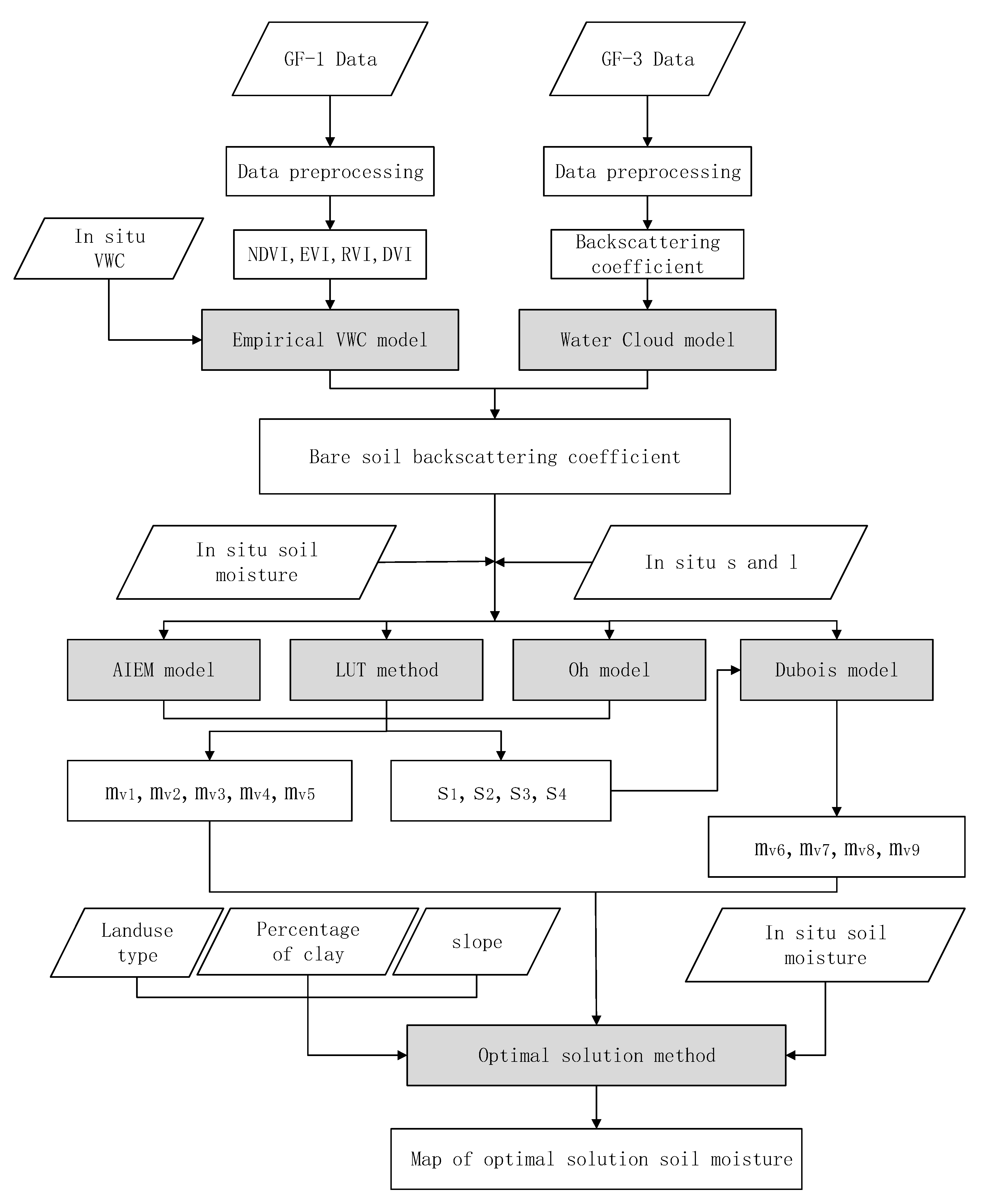
In situ measurements were conducted from 17 to 19 of October 2018, simultaneously with the GF-3 and GF-1 acquisitions. During the in-situ measurements, no evident changes in the temperature or precipitation were found in the study area. A total of 94 soil samples were selected from this area. The position of each sample field was identified and recorded by Global Positioning System (GPS). Figure 2 shows the map of the sampling sites and details regarding the soil moisture samples.

The entire study area was classified on the basis of three strategies, each containing 4–5 classes (listed in

Table 1. Detailed information of the 94 samples taken from a study area in Jiangsu Province, China.

	Type Class	Number of Samples	Proportion of Total Samples (%)	Proportion of This Class in the Entire Study Area (%)
Land Use Type	Farmland	63	67.02	68.62
	Forest and shrub	25	26.60	30.51
	Grassland	4	4.26	0.84
	Bare land	2	2.13	0.03
Percentage Content of Clay (%)	14	1	1.06	0.67
	26	37	39.36	35.04
	28	26	27.66	35.94
	29	28	29.79	26.12
	37	2	2.13	2.23
Slope (°)	≤1	36	38.30	41.53
	1–2	32	34.04	28.47
	2–3	12	12.77	10.34
	3–4	7	7.45	5.02
	>4	7	7.45	14.64

). The number and proportion of sample points distributed in each class were counted to observe the difference between the proportion of sample points contained in a class and the proportion of this class in the total area of the study area [57]. As listed in the table, the proportion of sample points in a certain class is similar to the proportion of the class in the total area of the study area, indicating that the sampling is largely representative.

The soil moisture measurements were mainly acquired using time-domain reflectometry (TDR) probes for the top 5 cm in all the 94 sample fields, on the basis of the hypothesis that the factors affecting radar signal penetration, such as vertical inhomogeneity of soil moisture content at a depth of 0–5cm, could be ignored [42,56,58]. For each sample field, the probes were placed vertically, and three close-distance measurements (few meters apart) of the near-surface volumetric soil moisture were collected and averaged. Furthermore, a total of 29 samples were simultaneously collected, uniformly mixed, and placed in cutting rings and aluminum specimen boxes using the oven-drying method for the top 5 cm. These cutting rings and aluminum specimen boxes were weighed and recorded, and then transported back to the laboratory for drying in an oven at 108 ℃ for 24 h, until the boxes were completely dehydrated. The obtained gravimetric soil moisture (g/g) and soil bulk density (g/cm³) were used to calculate the volumetric soil moisture (cm³/cm³), which was used to calibrate the TDR measurements. A linear model was used to calibrate the volumetric soil moisture acquired by the TDR probes, and the result is shown in Figure 3. The calibrated values of the volumetric soil moisture ranged from 0.03 to 0.35 cm³/cm³, averaging at 0.19 cm³/cm³. A total of 60 soil moisture samplings were randomly selected as independent testing data, and the remaining samplings served as training data in different models and algorithms.

In this study, the root-mean-square (RMS) height and correlation length were measured as the roughness parameters using a needle profiler made of a 1 m-long board with 100 pins digitized at an interval of 1 cm, and a digital camera. At the sample fields, the needle profiler was inserted onto the soil surface in the east-west and north-south directions, and then two images were taken to record the roughness characteristics. The roughness values were calculated from the digitized curve based on the roughness images using a developed MATLAB program. The RMS height ranged from 0.3 to 1.7 cm, averaging at 1 cm. The correlation length ranged from 5 to 25 cm, with the average value of 15 cm. The results show that the microtopography of the study area is relatively flat. A total of 57 vegetation samples were collected and sealed in plastic black bags, in order to minimize the effects of photosynthesis and transpiration on the water content of the vegetation samples. The VWC (kg/m²) was calculated from the fresh and oven dried sampling measurements using the oven-drying method.

After fixing the drying process, the vegetation samples were dried in an oven at 65 °C, until the samples were completely dehydrated.

3. Methodology

In this study, a set of combined approach comprising a set of methods to obtain high-precision soil moisture, which integrate multi-source data, realize the coupling of commonly used models, and introduce background knowledge into the optimal solution method. The procedure of the methodology for soil moisture mapping, illustrated in Figure 4, is explained as follows:

In the first step, the influence of the vegetation canopy water content was removed from the total backscattering coefficients, and the backscattering coefficient of the bare soil was obtained. The specific operations were as follows: first, an empirical VWC model was established using four vegetation indices extracted from the GF-1 satellite data and measured vegetation canopy water content data, and the accuracy of this empirical model was then compared with that of the conventional one-variable quadratic model; second, a WCM with localized parameters was established using the HH and VV polarization backscattering coefficients extracted from the GF-3 satellite data and in situ experimental data, and the accuracy of this model was compared with that of a model that uses empirical parameters.

In the second step, four commonly used soil moisture inversion models were coupled, and a total of nine soil moisture maps were obtained. The specific operations were as follows: five maps of the soil moisture and four RMS height maps were obtained using the AIEM model, Oh model, and look-up table (LUT) method; the four RMS height maps were then taken as input data for the Dubois model, and four soil moisture maps were obtained.

In the third step, based on the above nine soil moisture maps, a strategy of pixel classification and algorithm selection was applied to draw the optimal solution soil moisture map based on background knowledge. The specific operations were as follows: first, the study area was divided into several categories based on a certain background knowledge, each of which was assigned one of the nine algorithms with best precision. The results of all the categories were then combined to form a soil moisture map of the entire study area; finally, the three soil moisture maps based on the three sets of background knowledge were compared, and one with the best precision was selected as the optimal solution soil moisture map.

3.1. Vegetation Effect Correction Models

The empirical VWC model and WCM with localized parameters were applied to remove the vegetation effects from the total backscattering coefficient. The reason for constructing an empirical VWC model considering four vegetation indices is as follows: Although most of the study area is farmland, the underlying surface of the farmland is relatively complex, so it is likely that the VWC of the complex vegetation types cannot be accurately described by any single vegetation index; furthermore, a total of 57 VWC samples were collected during the in situ experiment, and the measured data were fully utilized in the process of constructing an empirical model that was more suitable for the study area. Similarly, the WCM with localized parameters makes full use of the in- situ experiment. To make the results more convincing, the accuracies of the empirical VWC model and WCM with localized parameters were compared with those of the conventional one-variable quadratic model and WCM with empirical parameters.

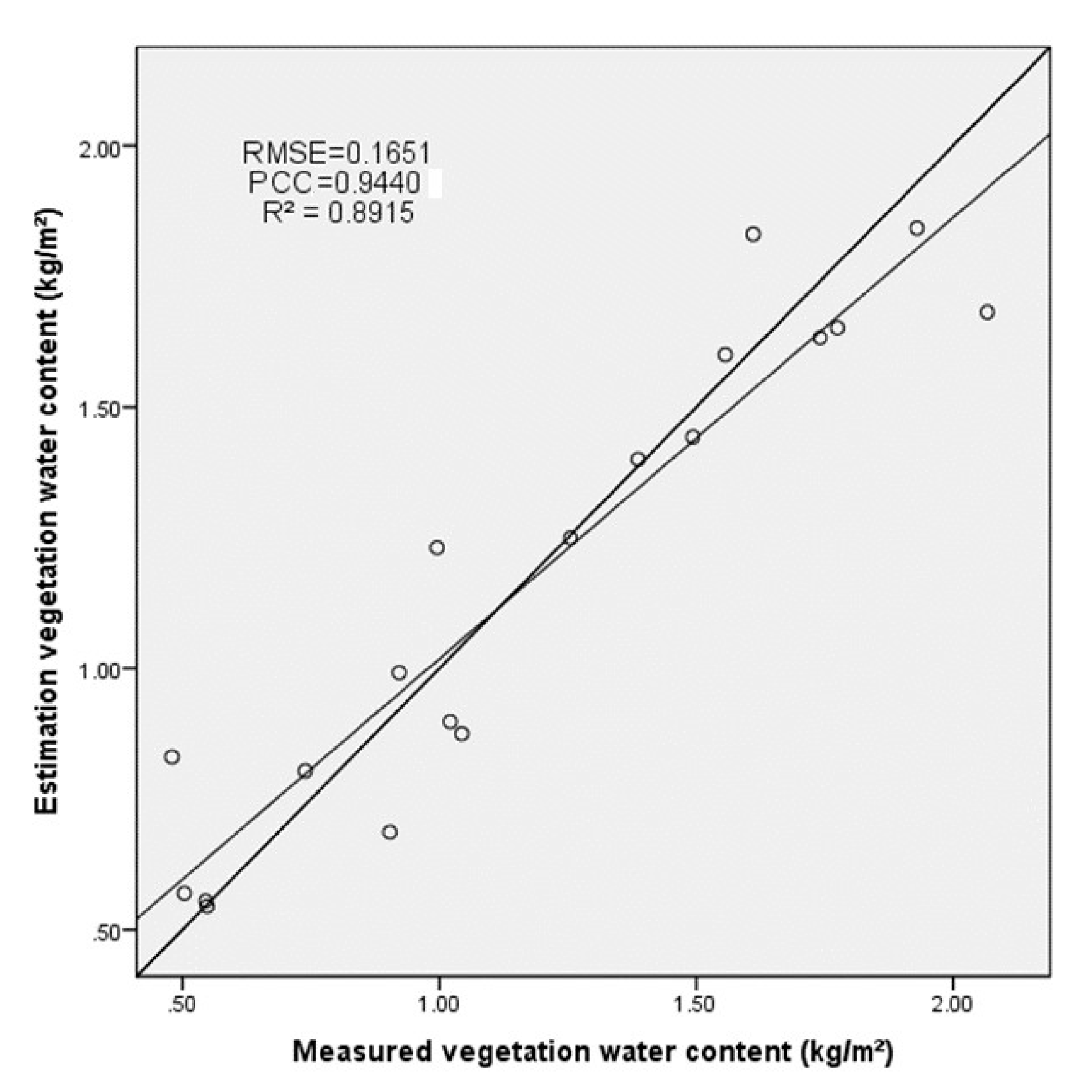
3.1.1. Vegetation Water Content Estimation Model

The VWC is an important parameter in the WCM. To eliminate the influence of vegetation canopy on the total backscattering coefficient, the VWC should be estimated. Because of the time and economic costs, it is difficult to acquire the VWC via ground tests on a large scale. Fortunately, the development of remote sensing technology has led to an effective solution to this problem. Published studies confirmed that the VWC has a significant correlation with the vegetation indices obtained from remote sensing datasets [55,56,57,58,59,60]. The vegetation indices often used to estimate the VWC include the normalized difference vegetation index (NDVI), normalized difference water index (NDWI), enhanced vegetation index (EVI), difference vegetation index (DVI), and ratio vegetation index (RVI) [61,62,63,64].

The GF-1 wide-field-view data synchronized with the GF-3 data passing time were used to calculate the vegetation indices. Considering the configuration of the GF-1 satellite, four vegetation indices were selected for the calculation: the NDVI, EVI, RVI, and DVI. These were calculated as follows:

$$\mathrm{NDVI}=\frac{NIR-RED}{NIR+RED}$$

(1)

$$\mathrm{EVI}=2.5\times \frac{NIR-RED}{NIR+6.0RED-7.5BLUE+1}$$

(2)

$$\mathrm{RVI}=\frac{NIR}{RED}$$

(3)

$$\mathrm{DVI}=\mathit{NIR}-\mathit{RED}$$

(4)

where NIR is the reflectivity at the near-infrared band; RED is the reflectivity at the red band; BLUE is the reflectivity at the blue band.

Previous works have indicated that the one-variable quadratic models, along with the linear and exponential models, are suitable for describing the correlation between the vegetation indices and VWC [55,61,62,63]. However, in most studies, only one of the vegetation indices (such as the NDVI) with the strongest correlation with the VWC was used in the calculation [61]. For medium-scale research areas with a complex surface cover, a combination of multiple vegetation indices may be more effective and accurate.

In this study, we developed a new empirical model in which all the four vegetation indices were incorporated in the calculation. Moreover, the accuracy of the new model was compared with those of the four one-variable quadratic models with each vegetation index, so as to verify the efficiency of the new model. The one-variable quadratic models used for accuracy comparison and the new model can be described as follows:

$$VW{C}_{VI}=\mathrm{a}\times V{I}^2+b\times VI+c$$

(5)

where $VW{C}_{VI}$ is the VWC calculated using the one-variable quadratic model (kg/m²); VI is the vegetation index obtained from the GF-1 satellite data; a, b, and c are the empirical parameters obtained using the least-squares method.

Each vegetation index has a certain scope of application and works well only under a certain growth condition, so a VWC model constructed using only a single vegetation index may not effectively reflect the condition of the entire study area. Considering the diversity of the vegetation types in the study area, a combined model incorporating the four vegetation indexes was developed. The 1stOpt software was used in the process of constructing the combined model, and the fitting accuracy and number of parameters were considered. The combined model can be expressed as follows [59]:

$$\mathrm{VWC}=d+e\times NDVI\times RVI+f\times NDVI\times EVI+g\times DVI\times EVI+h\times RVI\times EVI$$

(6)

where VWC is the VWC calculated using the new empirical model (kg/m²); NDVI, EVI, DVI, and RVI are the vegetation indices obtained from the GF-1 satellite data; d, e, f, g, and h are the empirical parameters obtained using the least-squares method.

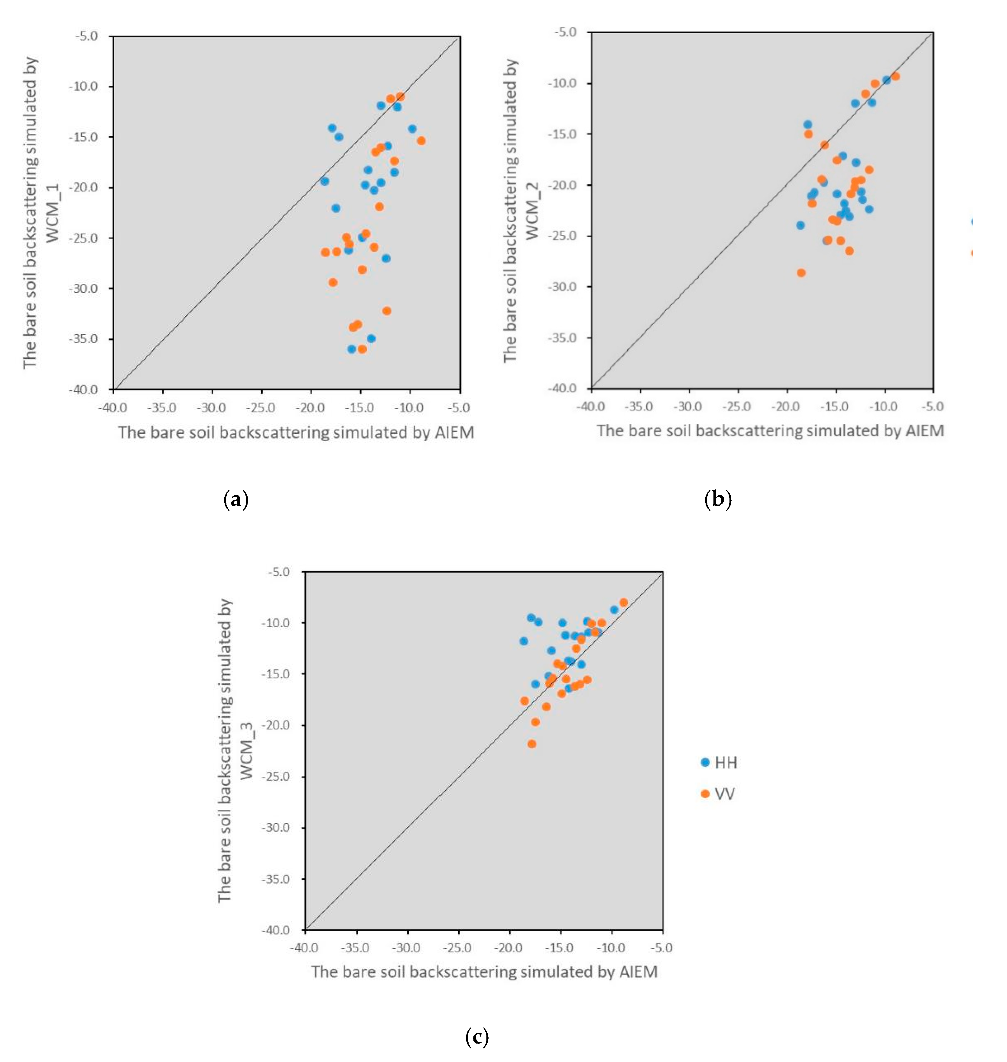
3.1.2. Water-Cloud Model

The backscattering coefficient obtained from the study area is affected by the land surface and radar configuration parameters [27,31]. In this study, the radar configurations were obtained from the head file of the GF-3 SAR sensor. Therefore, only the influences of land surface parameters were considered, including the soil moisture, roughness, and vegetation. To extract the backscattering of the bare soil surface, which is directly correlated to the soil moisture, the effect of vegetation canopy should be removed.

To describe the backscattering of the soil and vegetation in the vegetation-covered soil surfaces, a semi-empirical WCM, first developed by Attema and Ulaby [31], has been widely used as the vegetation impact correction model. The WCM is based on the following basic assumptions: (1) The vegetation canopy is represented as a homogeneous horizontal water cloud of identical and uniformly water spheres. (2) The multiple scattering between the canopy and soil is ignored. (3) The only significant variables in the model are the height of the canopy layer and cloud density, and the latter is assumed to be proportional to the volumetric VWC of the canopy [31].

For a given incidence angle, the classic WCM can be expressed as follows:

$${\sigma }^0={\sigma }_{veg}^0+{\tau }^2\times {\sigma }_{soil}^0$$

(7)

$${\tau }^2=\exp \left(-2\times B\times VWC/\cos \theta \right)$$

(8)

$${\sigma }_{veg}^0=\mathrm{A}\times VWC\times \cos \theta \times \left(1-{\tau }^2\right)$$

(9)

where ${\sigma }^0$ is the total backscattering coefficient, considering the incoherent sum of the contributions of the vegetation and underlying soil (dB), ${\sigma }_{veg}^0$ is the backscattering coefficient of the vegetation canopy (dB), ${\sigma }_{soil}^0$ is the direct backscattering coefficient of the underlying soil surface (dB), ${\tau }^2$ is the two-way transmissivity of the vegetation, VWC is the vegetation water content (kg/m²), $\theta$ is the incident angle (°), and A and B are parameters depending on the vegetation type. There is no general theoretical basis to obtain the values of A and B, which are typically determined by fitting the WCM against experimental datasets.

The original WCM has been subsequently modified or extended by various researchers [27]. Bindlish and Barros showed that the accuracy of the WCM could be improved by considering the radar-shadow effect. The concept of a dimensionless vegetation correlation length was used to better describe the geometric effect of the vegetation spacing; this parameter is similar to the surface correlation length used in the AIEM [59]. It can be interpreted as the distance at which the plants are considered independent scatterers [60]. Based on the improved WCM, Equations (10) and (11) must be modified to correct for the radar-shadow effect. The modified total backscattering coefficient and vegetation effect can be expressed as follows:

$${\sigma }^0={\sigma }_{veg}^{*}+{\tau }^2\times {\sigma }_{soil}^0$$

(10)

$${\sigma }_{veg}^{*}={\sigma }_{veg}^0\times \left[1-exp\left(-\alpha \right)\right]$$

(11)

where ${\sigma }_{veg}^{*}$ is the modified vegetation contribution, and $\alpha$ is the radar-shadow coefficient parameter, which is also considered the dimensionless vegetation correlation length.

In this study, three different WCM experiments were conducted: in the first case, the classic WCM was used, and the empirical parameters A and B were recorded as 0.0012 and 0.091, respectively, based on the values reported by Bindlish [60] (WCM_1). In the second case, the same classic WCM was used; however, the empirical parameters A and B were obtained using the least-squares method with the in situ experimental datasets (WCM_2). In the third case, an improved WCM considering the radar-shadow effects was selected; the empirical parameters A, B, and $\alpha$ were calculated using the least-squares method (WCM_3) with the in situ experimental datasets.

3.2. Soil Moisture Content Retrieval Model

To convert the bare soil backscattering coefficient to the soil moisture content, four commonly used inversion models (AIEM model, LUT method, Oh model, and Dubois model) were coupled. In this section, only the general principles and formulae of these models are introduced. A more detailed discussion of the relevant techniques and theory can be found in the references mentioned in this section.

The process of coupling the four models involved five steps. Only the general principles of these models are introduced in this section, and since steps 2 and 3 involve the analysis and application of the results generated in the intermediate process, the details of these are described in Section 4.2.

Step 1: The AIEM-simulated database was generated using the AIEM model, based on the in situ datasets and GF-3 configuration.

Step 2: Based on the AIEM-simulated database obtained in step 1, the responses of the bare soil backscattering coefficients and input parameters were analyzed, and the relationship structure between the soil moisture and input parameters was then determined. Thereafter, the empirical model was constructed using the measured soil moisture and bare soil backscattering coefficient; this model was used as an algorithm to map the soil moisture (m_v1).

Step 3: Similarly, based on the AIEM-simulated database, the LUT method was established using tree cost functions, which generate three soil moisture maps (m_v2, m_v3, and m_v4) and three RMS height results (s1, s2, and s3).

Step 4: In parallel with the above three steps, based on the in-situ database and backscattering coefficient, the Oh model was used to map the soil moisture (m_v5), along with the RMS height result (s4).

Step 5: After the above four steps, a total of four RMS height results were obtained, which were used as input data to the Dubois model. Based on the backscattering coefficient and measured soil moisture, four soil moisture maps (m_v6, m_v7, m_v8, and m_v9) were obtained corresponding to the four RMS height results.

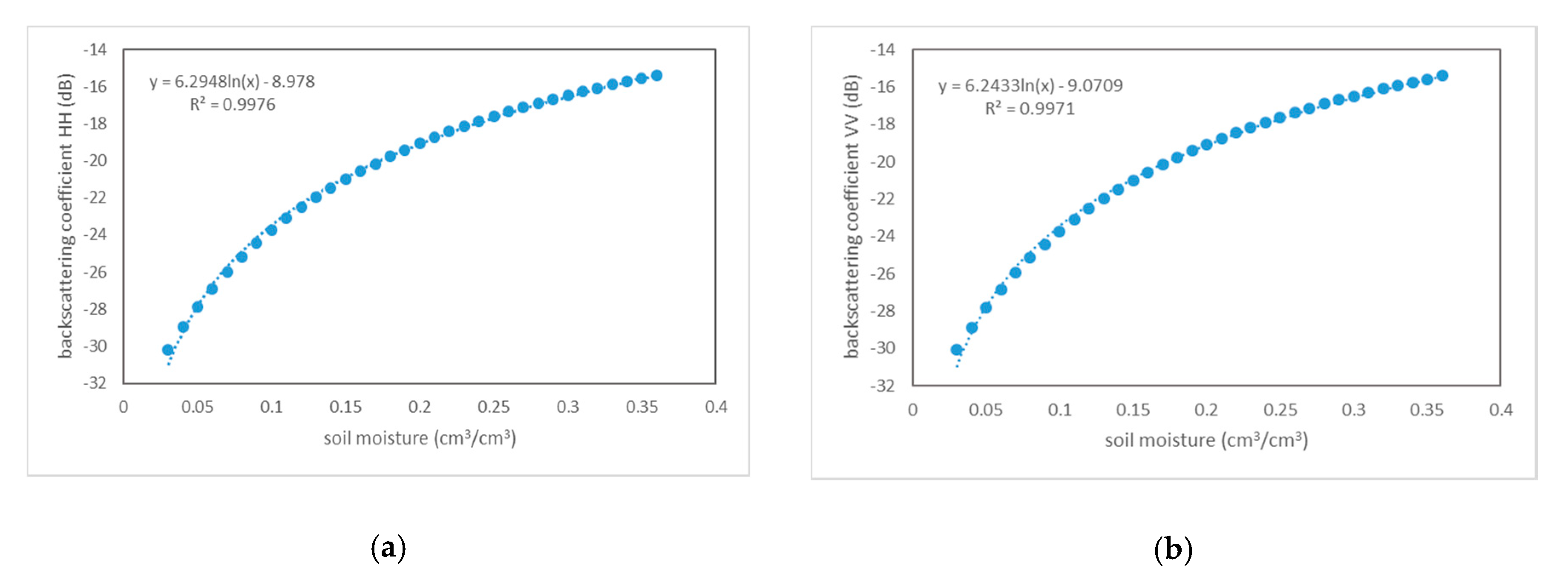
3.2.1. Estimated Model Constructed by AIEM

The AIEM model was developed by Chen and Wu in 2003 based on the classic IEM [35,36,37]. The AIEM is a well-established theoretical model in which the discontinuities in the surface roughness and Fresnel reflection coefficient were resolved by replacing the Fresnel reflection coefficients with a transition function [37,38,65]. Extensive experimental datasets were used to analyze the accuracy and validity of this model, the results of which indicated that the AIEM could accurately simulate the backscattering coefficients under a wide range of conditions [38,66].

In this study, the AIEM was adopted to establish a simulated database, and the responses of the bare soil backscattering coefficients, incident angle, roughness parameter, soil dielectric constant, and frequency were simulated under the configuration of the GF-3 sensor. The soil dielectric constant simulated from the AIEM was converted to the soil moisture via the dielectric-mixed Dobson model [67]. The frequency of the GF-3 sensor was fixed at 5.4 GHz, and other input parameters based on in situ data are as listed in

Table 2. Values of the input parameters to the AIEM model.

Input Parameters	Minimum	Maximum	Interval
Incidence angle (°)	30	60	1
RMS height (cm)	0.3	1.8	0.1
Correlation length (cm)	5	25	1
Soil moisture (vol. cm³/cm³)	0.03	0.36	0.01

.

Considering the difficulties in simulating the bare soil backscattering coefficients in cross-polarization using the AIEM, only the backscattering coefficients simulated in HH and VV polarizations were used in this study. Based on the AIEM and Dobson model, the equations of the bare soil backscattering coefficients can be expressed as follows:

$${\sigma }_{PP}^0=f\left(\theta ,f,s,l,m_v\right)$$

(12)

where $\theta$ is the incidence angle, $f$ is the frequency of the GF-3 sensor, $s$ is the RMS height, $l$ is the correlation length, and $m_v$ is the bare soil moisture content.

3.2.2. LUT Inversion Method

The LUT of the HH and VV polarization backscattering coefficients was obtained from previous studies [37,38]. In this study, the LUT method was used to obtain soil moisture and root mean square (RMS) height at the same time. It was based on the AIEM-simulated database, and under the configuration of GF-3 satellite, each record of the database contains five interrelated parameter values, including backscattering coefficient, root mean square (RMS) height, correlation length and soil moisture. For a particular pixel of the bare soil backscattering coefficient map, a specific record in the simulated database could be located by minimizing the cost function, and the soil moisture and root mean square (RMS) height in this record were extracted as the best-fit inversion value corresponding to the backscattering coefficient of the pixel.

Three cost functions were established to retrieve the bare soil moisture in this study:

$$Z_1=min\left(\sqrt{{\left({\sigma }_{HH}^0-{\sigma }_{HH\_AIEM}^0\right)}^2}\right)$$

(13)

$$Z_2=min\left(\sqrt{{\left({\sigma }_{VV}^0-{\sigma }_{VV\_AIEM}^0\right)}^2}\right)$$

(14)

$$Z_3=min\left(\sqrt{{\left({\sigma }_{HH}^0-{\sigma }_{HH\_AIEM}^0\right)}^2+{\left({\sigma }_{VV}^0-{\sigma }_{VV\_AIEM}^0\right)}^2}\right)$$

(15)

where ${\sigma }_{HH}^0$ and ${\sigma }_{VV}^0$ are the HH and VV polarization backscattering coefficients (dB) obtained from the bare soil backscattering images, respectively, and ${\sigma }_{HH\_AIEM}^0$ and ${\sigma }_{VV\_AIEM}^0$ are the HH and VV polarization backscattering coefficients (dB) in the AIEM-simulated database, respectively.

3.2.3. Semi-Empirical Oh Model

Oh et al. proposed several versions of the semi-empirical polarimetric models between 1992 and 2004 [37,39]. The Oh model is based on physical theoretical models, and the relevant parameters in this model were obtained as field experimental data using several polarimeter radar scatterometers [39,68]. The latest version of the Oh model modified in 2004 contains a new equation that ignores the correlation length, built on the previous version [37]. This improvement was made on the basis of the results of a published research, which indicated that the ratio q (${\sigma }_{HV}^0/{\sigma }_{VV}^0$) is not sensitive enough to the roughness parameters and that the measurement of the correlation length may vary depending on the scale of the instrument used [39].

In this study, a new expression for the Oh model (2004) was used to estimate the soil moisture of the bare soil. The input parameters of the Oh model (2004) include the incidence angle, wavenumber, RMS height, and soil moisture or dielectric constant. The 2004 version of the Oh model can be expressed as [37,39]:

$${\sigma }_{VH}^0=0.11\times m_v^{0.7}\times {\left(cos\theta \right)}^{2.2}\times \left[1-exp\left(-0.32\times {\left(ks\right)}^{1.8}\right)\right]$$

(16)

$$\mathrm{p}\equiv \frac{{\sigma }_{HH}^0}{{\sigma }_{VV}^0}=1-{\left(\frac{\theta }{{90}^{°}}\right)}^{0.35\times m_v^{-0.65}}\times exp\left[-0.4\times {\left(ks\right)}^{1.4}\right]$$

(17)

$$\mathrm{q}\equiv \frac{{\sigma }_{VH}^0}{{\sigma }_{VV}^0}=0.095\times {\left(0.13+sin1.5\theta \right)}^{1.4}\times \left\{1-exp\left[-1.3\times {\left(ks\right)}^{0.9}\right]\right\}$$

(18)

where p is the co-polarized ratio, q is the cross-polarized ratio, ${\sigma }_{VH}^0$ represents the backscattering coefficients for VH polarization (dB), and $ks$ is the RMS height normalized to the wavelength (k is the wavenumber). The dataset in this study satisfies the validity range of the Oh model (2004) (0.04–0.29 cm³/cm³ for $m_v$, 0.13–6.98 for $ks$, and 10–70° for $\theta$) [37].

3.2.4. Semi-Empirical Dubois Model

The Dubois model was developed in 1995 using scatterometer data for retrieving the soil moisture content and RMS height from the remote sensing radar data [37]. The Dubois model has been applied in some studies, with satisfactory accuracy [40,41]. The validity domain of the model is $m_v$ < 0.35 cm³/cm³ and $ks$ ≤ 2.5, $\theta$ ≥ 30°. The equations applicable to HH and VV polarization data are:

$${\sigma }_{VV}^0={10}^{-2.35}\times \frac{{\cos }^3\theta }{{\sin }^3\theta }\times {10}^{0.046\times \epsilon \times \tan \theta }\times {\left(ks\times \sin \theta \right)}^{1.1}\times {\lambda }^{0.7}$$

(19)

$${\sigma }_{HH}^0={10}^{-2.75}\times \frac{{\cos }^{1.5}\theta }{{\sin }^5\theta }\times {10}^{0.028\times \epsilon \times \tan \theta }\times {\left(ks\times \sin \theta \right)}^{1.4}\times {\lambda }^{0.7}$$

(20)

where $\epsilon$ is the dielectric constant, and $\lambda$ is the radar wavelength.

In this study, the Dubois and Dobson models were combined to complete the following processes: the RMS height map obtained using the Oh model and LUT inversion method was used as the input data, and the soil dielectric constant was generated using the Dubois model based on the HH and VV polarization backscattering coefficients, which were converted to the soil moisture content using the dielectric-mixed Dobson model.

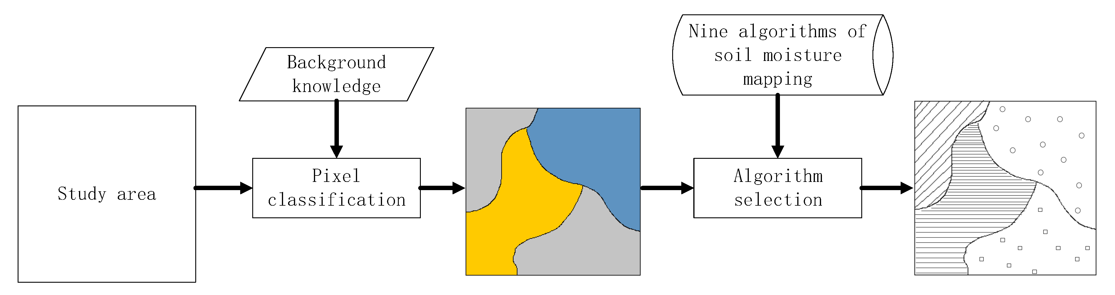
3.3. Optimal Solution Method

This section presents a simple and effective optimal solution method used to select and combine the nine soil moisture mapping algorithms proposed above based on three types of background knowledge. Figure 5 shows the overall process of the optimal solution method.

For a specific background knowledge, the pixels in the study area were classified into several categories using the classification strategy constructed based on this knowledge, and the algorithm with the highest accuracy was selected in terms of the evaluation index. The algorithm results corresponding to each category were calculated independently. Thereafter, the calculation results of all the categories were combined to form the soil moisture map of the entire study area.

A total of three spliced maps of the soil moisture were obtained using three classification strategies. Finally, these maps were compared, and the one with the best accuracy was selected as the optimal solution soil moisture map of the study area.

Three optimal solution classification strategies were proposed as follows: (1) Based on the four main land use types (farmland, grassland, shrub, and bare land) in the study area, a statistical analysis was made on the accuracy of the nine soil moisture inversion maps, and the best inversion method for each type was selected; (2) Based on the percentage of clay, nine soil moisture inversion accuracies were calculated corresponding to the five clay percentage values (14, 26, 28, 29, and 37%), and the best inversion method was selected for each type; (3) Similarly, based on the slope levels of the study area, a statistical analysis was made on the accuracies of the nine soil moisture inversion maps under five slope levels (Level 1: ≤1°; Level 2: 1–2°; Level 3: 2–3°; Level 4: 3–4°; Level 5: ≥4°), and the inversion method with the highest accuracy for each slope level was selected as the optimal solution method.

The equation of the optimal solution methods is expressed as follows:

$$m_v=f\left(m_{v1},m_{v2},\dots \dots ,m_{v9}\right)$$

(21)

where $m_{vn}$ is the retrieved moisture based on the four models.

4. Results and Discussion

4.1. Vegetation Effect Correction

This section presents the results of the calculation parameters of the empirical VWC model and WCM with localized parameters. To prove the superiority of the two models compared with the commonly used empirical models and empirical parameters, we developed conventional one-variable quadratic models and WCM with empirical parameters for comparative experiments. The comparison results are given in this section.

The developed empirical model was used to retrieve the VWC from the GF-1 vegetation indices, compared with the one-variable quadratic model. The agreement between the measured VWC and the modeled VWC was evaluated on the basis of the Pearson correlation coefficient (PCC).

Table 3. Parameters of the VWC model and the PCC based on the 19 validation sample datasets.

VWC model	Empirical Parameters							PCC
	a		b			c
VWCNDVI	26.0820		−1.8558			1.0915		0.9158
VWCEVI	4.6957		1.4673			0.9790		0.9054
VWCRVI	1.3854		−1.7960			1.3724		0.9124
VWCDVI	46.9080		5.8157			0.9459		0.8805
VWC	d	e		f	g		h	0.9442
	1.1604	4.3773		18.2684	14.1764		−4.8787

lists the coefficient of determination values based on 19 validation sample datasets.

From Table 3, we find that by comparing the performances of the four vegetation indices in the one-variable quadratic models, VWC_NDVI provides a higher accuracy than the other vegetation index models (PCC = 0.9158). However, the accuracy of the VWC estimated from the combined vegetation model was significantly higher than those estimated from any one of the one-variable quadratic models (PCC = 0.9442).

The VWC was estimated using GF-1 satellite data. As shown in Figure 6, the PCC between the estimated and measured VWC values is 0.9440, the root-mean-square error (RMSE) of the estimated VWC is 0.1651 kg/m², and the coefficient of determination (R²) is 0.8915. The correlation between the measured and estimated VWC values was significant at the 0.01 level.

Three different WCM experiments were conducted using the results of the above VWC. As mentioned previously, the classic WCM was used, and the empirical parameters A and B were recorded as 0.0012 and 0.091, respectively (WCM_1); in the second case, the same classic WCM was used; however, the empirical parameters A and B were obtained using the least-squares method with the in situ experimental datasets (WCM_2); in the third case, the improved WCM considering the radar-shadow effects was selected, and the empirical parameters A, B, and $\alpha$ were calculated using the least-squares method (WCM_3) with the in situ experimental datasets. The values of the empirical parameters used in the WCM were recorded by referring to published works or calculated based on the in situ experimental datasets. The AIEM model was used to simulate the bare soil backscattering at each sampling location where in situ experimental data of the soil moisture and auxiliary data were available.

To evaluate the validity of the three WCM experiments conducted on the vegetation effect correction in the GF-1 and GF-3 satellite configurations, the bare soil backscattering simulated using the WCM was compared with that simulated using the AIEM, in Figure 7.

Based on the analysis of the comparative experimental results, we find that the empirical VWC model and WCM with localized parameters considering the radar-shadow effects do have evident accuracy advantages, confirming that the accuracy of the calculated bare soil backscattering coefficient could be ensured.

4.2. Bare Soil Moisture Estimation Based on Four Commonly Used Models

The process of coupling the four commonly used models included the five steps described in Section 3.2. In this section, Section 4.2.1, Section 4.2.2, Section 4.2.3 and Section 4.2.4 correspond to steps 2–5, respectively. Because steps 2 and 3 involve the analysis and application of the results generated in the intermediate process, they will be analyzed in more detail.

4.2.1. Bare Soil Moisture Estimation Based on AIEM

To build the bare soil moisture empirical estimation model based on the AIEM and map the soil moisture content, three steps were carried out. First, the responses of the backscattering coefficient and input parameters were analyzed to support the judgment of the structure of the inversion model; second, the parameters of this model were calculated based on the in situ experimental data; third, the soil moisture content in the entire area was mapped based on the model.

The input parameters of the AIEM include the radar system parameters and surface parameters of the study area. In the GF-3 radar sensor configuration, the frequency and incidence angle of the radar system parameters can be obtained from the header file. Therefore, only the responses of the bare soil backscattering coefficients and surface parameters of the study area were mainly considered in this study.

At a frequency of 5.4 GHz and an incident angle of 37°, the AIEM was used to generate a simulated database of the changed soil moisture conditions with a fixed roughness parameter value. Two conditions were required to be analyzed: first, the correlation length was considered a fixed value (15 cm), and the RMS height was considered a fixed-interval parameter (0.3, 0.6, 0.9, 1.2, 1.5, and 1.7 cm); second, the RMS height was considered a fixed value (1.0 cm), and the correlation length was considered a fixed-interval parameter (5, 10, 15, 20, and 25 cm). Figure 8 shows the results. The following rules can be summarized from this figure: First, When the roughness parameter is fixed, there is an evident nonlinear relationship between the soil moisture and the soil backscattering coefficients, the trends of which do not vary with the roughness interval parameter. With the increase in the soil moisture, the trend in the soil backscattering coefficient is upward, and the growth rate gradually decreases with an increase in the soil moisture.

Second, when the correlation length is fixed, the soil backscattering coefficient increases with the increase in the RMS height, and the increase amplitude gradually flattens with the increase in the RMS height. Third, at a fixed RMS height value, the soil backscattering coefficient decreases with the increase in the correlation length; however, the change trend is not as evident as the trends in the soil backscattering coefficients and RMS height. Fourth, under the same parameter conditions, the soil backscattering coefficient value for the HH polarization is slightly lower than that for the VV polarization.

At a frequency of 5.4 GHz and an incident angle of 37°, the AIEM was used to create a database for two conditions: first, the correlation length was considered a fixed value (15 cm), and the soil moisture was considered a fixed-interval parameter (0.03, 0.09, 0.15, 0.21, 0.27, and 0.33 cm³/cm³); second, the RMS height was considered a fixed value (1.0 cm), and the soil moisture condition was the same as in the first case. The responses of the roughness parameter and bare soil backscattering coefficient could be analyzed based on the database.

The following rules can be summarized from Figure 9: First, at a fixed soil moisture value, the backscattering coefficient decreases with the increase in the correlation length, whereas it increases with the increase in the RMS height.

Second, the sensitivity of the backscattering coefficient to the correlation length declines with the increase in the soil moisture.

Third, the soil backscattering coefficients are highly sensitive to the RMS height and tend to decrease with the increase in the soil moisture; however, this trend is not as evident as the change tendency in the correlation length.

Fourth, at a fixed soil moisture value, the soil backscattering coefficients gradually decrease with the increase in the RMS height; the change range gradually decreases, and the curve tends to flatten.

For a fixed sensor configuration, the soil backscattering coefficient is mainly affected by the roughness parameter and soil moisture. As shown in Figure 9, there is a significant nonlinear relationship between the soil backscattering coefficient and surface parameter for both the polarizations. In this section, based on the above qualitative analysis, a quantitative estimation model is presented and verified.

The effects of the roughness parameter and soil moisture on the soil backscattering coefficient are considered independent of each other, based on published studies [9,42]. In this study, the quantitative relationship between the soil backscattering coefficient and surface parameter could be described as the sum of the contributions of the roughness and soil moisture.

The first step is to establish a quantitative relationship between the soil backscattering coefficients and two roughness parameters based on the AIEM-simulated database for an average value (0.19) of the soil moisture from the in-situ datasets. For a quantitative model, the greater the number of roughness parameters, the greater the uncertainty in the model [64]. Therefore, a combined roughness parameter that combines the correlation length and the RMS height into one comprehensive parameter is selected. The combined roughness parameter has been widely used in previous studies for soil moisture estimation [9,37,69]. The results of these studies show that the new roughness parameter can help characterize the natural surface roughness conditions, while reducing the uncertainty of the estimation model. Under the different conditions of study areas and sensor configurations, the form of the combined roughness parameter can be different. In this study, three forms of the combined roughness parameter were tested to select the most suitable one for the surface conditions. Based on the database simulated using the AIEM, a multivariate regression analysis of the three forms of the combined roughness parameter and the soil backscattering coefficient was performed using the 1stOpt software.

Table 4. Quantitative relationship between the three forms of combined roughness parameters and the soil backscattering coefficient.

Combined Roughness Parameter	Formula	PCC	References
$Z_{S1}=\mathrm{S}/\mathrm{L}$	${\sigma }_{HH}^0=9.0421+13.0996\times \ln \left(Z_{S1}\right)$	0.8070	[9]
	${\sigma }_{VV}^0=6.8906+12.0569\times \ln \left(Z_{S1}\right)$	0.8339
$Z_{S2}=S^2/\mathrm{L}$	${\sigma }_{HH}^0=-1.7147+8.7825\times \ln \left(Z_{S2}\right)$	0.9579	[70]
	${\sigma }_{VV}^0=-3.2885+7.9854\times \ln \left(Z_{S2}\right)$	0.9659
$Z_{S3}=S^3/\mathrm{L}$	${\sigma }_{HH}^0=-8.3608+6.1922\times \ln \left(Z_{S3}\right)$	0.9629	[71]
	${\sigma }_{VV}^0=-9.4118+5.6029\times \ln \left(Z_{S3}\right)$	0.9680

lists the results. From Table 4, we find that there is a significant logarithmic relationship between the three forms of the combined roughness parameter and the soil backscattering coefficients. The PCC of all the constructed equations is greater than 0.8.

In contrast, the equations based on $Z_{S3}$ give the highest precision for both HH (0.9629) and VV (0.9680) polarizations. Therefore, the form of $Z_{S3}$ was used as $Z_S$ in this study, to characterize the combined effect of the correlation length and RMS height. Figure 10 shows the corresponding relationship between $Z_S$ and the soil backscattering coefficient under different soil moisture conditions.

The functional expressions between the soil moisture and the backscattering coefficients for a correlation length of 15 cm and an RMS height of 1 cm based on the simulated database are shown in Figure 10. The R-square of the regression equations for both HH and VV polarizations is greater than 0.99.

According to Figure 10, the effect of soil moisture on soil backscattering coefficients under the condition of fixed roughness parameters can be expressed as follows:

$${\sigma }_{HH}^0=-8.9780+6.2948\times \ln \left(m_v\right)$$

(22)

$${\sigma }_{VV}^0=-9.0709+6.2433\times \ln \left(m_v\right)$$

(23)

Based on the above analysis, for a fixed frequency and incident angle, the expression of the quantitative model can be written as:

$${\sigma }_{HH}^0=-17.3388+6.2948\times \ln \left(m_v\right)+6.1922\times \ln \left(Z_s\right)$$

(24)

$${\sigma }_{VV}^0=-18.4827+6.2433\times \ln \left(m_v\right)+5.6029\times \ln \left(Z_s\right)$$

(25)

Combining Equations (24) and (25), the soil moisture can be estimated mathematically, and the general expression is as follows:

$$m_v=\exp \left(i\times {\sigma }_{VV}^0+j\times {\sigma }_{HH}^0+k\right)$$

(26)

where $i$, $j$, and $k$ are the empirical parameters. In this study, the empirical parameters were obtained using the least-squares method based on the in-situ datasets. The bare soil moisture estimation equation based on the in-situ experiments is as follows:

$$m_v=\exp \left(-0.0407\times {\sigma }_{VV}^0+0.0236\times {\sigma }_{HH}^0-2.0599\right)$$

(27)

The soil moisture map of the entire study area was obtained using this estimation model based on the backscattering coefficients for HH and VV polarizations.

4.2.2. Bare Soil Moisture Estimation Based on the Oh Model

The backscattering coefficients for the VV, HH, and VH polarizations used in the Oh model were obtained from the results of the vegetation effect correction model described in Section 4.1. The backscattering coefficients of urban land and water bodies are significantly different from those of bare soil [69,72,73]. Therefore, the threshold value summarized based on the datasets can be used to effectively mask the urban land and water bodies. For bare soil, the backscattering coefficient for VV polarization is always greater than that for HH polarization, and the latter is greater than that for VH polarization [37,39]. Based on the statistical analysis of the backscattering coefficients, we found the existence of pixels whose backscattering coefficients for HH polarization are higher than that for VV polarization. The reason for this phenomenon may be that, despite the high accuracy of the vegetation correction model, some pixels are still affected by the influence of sparse vegetation [37].

In this study, the pixels in the Oh model were screened based on the following conditions: First, the backscattering coefficients of the pixel are above the threshold value set for urban land and water bodies, summarized based on the datasets. Second, the backscattering coefficient of the pixel for VV polarization is greater than that for HH polarization. Lastly, the estimated soil moisture and $ks$ should meet the range of soil moisture condition of the Oh model: 0.04 cm³/cm³ < mv < 0.29 cm³/cm³, and 0.13 <$ks$ < 6.98.

4.2.3. Bare Soil Moisture Estimation Based on LUT

The LUT in this study was based on the AIEM-simulated database, described in Section 3.2.1, with fixed incidence angle (37°) and frequency (5.4 GHz) values under the configuration of GF-3 images. This LUT indicates the one-to-one correspondence relationship between the bare soil backscattering coefficients for HH and VV polarizations, roughness parameters, and soil moisture. The pixels of the bare soil backscattering-coefficient images, obtained in Section 4.1, were calculated using the cost functions one by one. When the cost function value ${\mathrm{Z}}_n$ (n = 1, 2, and 3) reached the minimum, the soil moisture value corresponding to ${\sigma }_{HH\_AIEM}^0$ and ${\sigma }_{VV\_AIEM}^0$ in the LUT was used as the best-fit inversion soil moisture value under the HH or VV polarization.

The results of the retrieved soil moisture content based on the cost functions Z₁, Z₂, and Z₃ show that the average soil moisture contents were 0.32, 0.29, and 0.30, respectively, with standard deviations of 0.05, 0.07, and 0.07, respectively.

4.2.4. Soil Moisture Estimation Based on Dubois Model

The four RMS height results retrieved from the LUT and Oh method were used in the Dubois model as input data to indirectly estimate the soil moisture. The inversion results of the soil moisture under the two polarization conditions could be obtained simultaneously in the Dubois model. After comparing their accuracies, we selected the HH polarization mode results of this model. Considering the limitation of the application conditions of the Dubois model, the pixels of the input and output images that do not meet the conditions were set as null values. Consequently, four soil moisture inversion maps were obtained.

4.2.5. Validation and Analysis of the Individual Soil Moisture Inversion Models

To evaluate the performance of the nine inversion soil moisture maps obtained using the most commonly used soil moisture models (AIEM, Oh model, LUT inversion model, and Dubois model), a validation experiment was conducted to confirm the agreement between the modeled soil moisture and the measured soil moisture in terms of the RMSE, PCC, mean absolute error (MAE), and bias. The RMSE and MAE could reflect the differences between the estimated and measured soil moisture values, where a low index value represents a high prediction accuracy. The positive and negative values of the bias could reflect the deviation direction. The PCC could reflect the linear correlation between the estimated and measured soil moisture values, where a value close to 1 represents a strong linear correlation.

Table 5. RMSE, MAE, PCC, and bias between the measured and estimated soil moisture values based on the validation dataset.

Inversion Models	RMSE (cm³/cm³)	MAE (cm³/cm³)	PCC	Bias (cm³/cm³)
$m_{v1}$	0.0321	0.0260	0.9115	−0.0150
$m_{v2}$	0.0538	0.0338	0.7441	−0.0117
$m_{v3}$	0.0769	0.0563	0.7287	−0.0426
$m_{v4}$	0.1059	0.0811	0.5679	0.0230
$m_{v5}$	0.0428	0.0306	0.8843	0.0174
$m_{v6}$	0.0710	0.0567	0.6551	−0.0420
$m_{v7}$	0.0687	0.0529	0.4114	0.0266
$m_{v8}$	0.0761	0.0608	0.6278	0.0107
$m_{v9}$	0.0676	0.0564	0.4599	−0.0141

lists the RMSE, MAE, PCC, and bias between the measured and estimated soil moisture values based on the 60 sample values from the validation dataset acquired during the in situ measurements. It should be noted that $m_{v1}$ represents the result of the estimation model based on the AIEM; $m_{v2}$,$m_{v3}$, and $m_{v4}$ represent the results of the LUT inversion model; $m_{v5}$ represents the results of the Oh semi-empirical model; $m_{v6}$,$m_{v7}$,$m_{v8}$, and $m_{v9}$ represent the results of the indirect soil moisture estimation method based on the Dubois model.

In terms of the RMSE and MAE, the estimation model constructed using the AIEM ($m_{v1}$: RMSE = 0.0321 cm³/cm³, MAE = 0.0260 cm³/cm³) was more accurate than the other models, followed by the Oh model ($m_{v5}$: RMSE = 0.0428 cm³/cm³, MAE = 0.0306 cm³/cm³) and the LUT inversion method under HH polarization ($m_{v2}$: RMSE = 0.0538 cm³/cm³, MAE = 0.0338 cm³/cm³). The indirect Dubois model combined with the Oh model ($m_{v9}$), combined with the LUT inversion method under VV polarization ($m_{v7}$) and the direct LUT inversion method under VV polarization ($m_{v3}$) gave moderate accuracy results, with an RMSE value lower than 0.077 cm³/cm³ and MAE value lower than 0.056 cm³/cm³. The accuracy of the LUT model for both HH and VV polarizations ($m_{v4}$) is relatively lower than those of the other inversion models.

The PCC could directly reflect the linear correlation between the estimated and measured soil moisture values. As listed in Table 5, the soil moisture estimated from the inversion model constructed using the AIEM ($m_{v1}$) had a strong linear relationship, with the PCC reaching 0.9115. The soil moisture calculated using the Oh model ($m_{v5}$) and LUT inversion method under HH or VV polarizations ($m_{v2}$ and $m_{v3}$) also had a good linear relationship with the measured values (PCC higher than 0.70). In contrast, there is no significant linear correlation between the results estimated using the indirect Dubois model combined with the Oh model ($m_{v9}$) and LUT inversion method under VV polarization ($m_{v7}$) and the measured soil moisture (PCC lower than 0.50).

The statistical analysis of the bias results shows that, among the nine inversion soil moisture maps, five models ($m_{v1}$, $m_{v2}$, $m_{v3}$, $m_{v6}$, and $m_{v9}$) show negative bias, indicating that the inversion results of these five models are generally higher than the measured soil moisture values; at the same time, four models ($m_{v4}$, $m_{v5}$, $m_{v7}$, and $m_{v8}$) show positive bias, indicating that these models give an overall underestimated result.

In summary, the evaluation and analysis results of the nine inversion maps on the validation dataset are as follows:

(1)

The estimation model constructed using the AIEM ($m_{v1}$) gives the highest accuracy for all the four verification indexes, followed by the Oh model ($m_{v5}$) and LUT inversion method under HH polarization ($m_{v2}$), whereas the accuracy of the LUT model for both HH and VV polarizations ($m_{v4}$) is relatively poor. The good performance of the estimation model constructed using the AIEM is attributed to the well-established theoretical model describing the radar scattering process, and at the same time, 37 sample datasets from the in-situ measurements were used as modeling data in establishing the regression model [9,42]. Previous studies have also shown that the Oh model is a highly accurate semiempirical model and that it is more favorable in the case of cross-polarized data for the inversion of complex surfaces [37,48]. However, because the model cannot express the soil moisture precisely for pixels with soil moisture below 0.04 or greater than 0.29, the precision of the model is compromised [69,70,74].

(2)

The RMS height, obtained from the LUT inversion method or Oh model, was used as input data for the Dubois model to estimate the soil moisture indirectly. In general, the indirect Dubois model ($m_{v6}$, $m_{v7}$, $m_{v8}$, and $m_{v9}$) has a relatively lower inversion accuracy than the direct inversion models ($m_{v1}$, $m_{v2}$, $m_{v3}$, $m_{v4}$, and $m_{v5}$). There are two possible reasons for this: first, significant errors exist in the process of RMS height inversion, which will be transmitted to the indirect inversion Dubois model; second, some factors, such as the residual vegetation effects and the row directional effects, may be taken as soil moisture fluctuation in the Dubois model [72,75].

(3)

Among the three LUT direct inversion methods ($m_{v2}$, $m_{v3}$, and $m_{v4}$), the differences between the estimated and measured soil moisture values are relatively minimum under HH polarization ($m_{v2}$: RMSE = 0.0538, MAE = 0.0338), followed by the inversion method under VV polarization ($m_{v3}$: RMSE = 0.0769, MAE = 0.0563). The linear correlation between the estimated and measured soil moisture values is acceptable under single polarization ($m_{v2}$ and $m_{v3}$), and the PCC values are greater than 0.7. This shows that the LUT inversion under single polarization is feasible to retrieve the soil moisture, consistent with previous results [37,40]. However, the accuracy of the direct or indirect LUT inversion under dual-polarization ($m_{v4}$ and $m_{v8}$) is unsatisfactory, inconsistent with a previous research by Zhang et al. [56]. The possible reason for the inconsistency is that the surface coverage of the study area in the previous research was monotonous, whereas in this study, the surface coverage was complex, and the vegetation types were varied, including a certain proportion of nurseries with evident body scattering effect.

4.3. Optimal Solution Method

Based on the nine soil moisture mapping algorithms, a simple and effective optimal solution method of pixel classification and algorithm selection was implemented, in order to obtain the most accurate soil moisture map. The principle and main steps of the optimal solution method have been described in detail in Section 3.3. In this section, the process and results of the algorithm selection, as well as the verification process of the accuracy of the spliced soil moisture maps, are described in detail.

In the last section, the accuracy of all the methods is verified and analyzed for the entire validation dataset. The overall analysis shows that the estimation model constructed using the AIEM ($m_{v1}$,) is the best, followed by the Oh model ($m_{v5}$) and LUT inversion method under HH polarization ($m_{v2}$). However, if the study area is divided into different categories based on background knowledge, the accuracy of the nine inversion maps in each category could be estimated differently, probably different from that of the overall analysis. In this study, three types of background knowledge data were used, including land use types, percentage content of clay, and slope levels.

The 30-m resolution land use data were downloaded from the website of Finer Resolution Observation and Monitoring Global Land Cover Products (http://data.ess.tsinghua.edu.cn/). The land use cover product is the first 30-m resolution global land cover map produced using Landsat Thematic Mapper and Enhanced Thematic Mapper Plus data. The soil texture data were downloaded from the Geographic Data Sharing Infrastructure, College of Urban and Environmental Science, Peking University (http://geodata.pku.edu.cn), and divided on the basis of three categories: the percentage of sand, percentage of silt, and percentage of clay. The slope levels were derived from the Shuttle Radar Topography Mission digital elevation model with a resolution of 30 m using the ArcGIS 10.2 software.

4.3.1. Construction of the Optimal Solution Method under Three Strategies

On the premise of introducing background knowledge to classify the study area, the soil moisture inversion method with the highest accuracy under each category was selected as the optimal solution method. In this study, three construction strategies for the optimal solution method were proposed based on the modeling dataset.

In strategy 1, the study area was divided into four categories based on the four main land use types. The soil moisture inversion map with the highest accuracy was selected as the optimal solution model for this certain land use type (

Table 6. Optimal solution strategy based on land use types and the accuracy of each algorithm (strategy 1).

Land Use Types	Optimal Model	RMSE (cm³/cm³)	MAE (cm³/cm³)	PCC	BIAS (cm³/cm³)
farmland	${\mathit{m}}_{\mathit{v}\mathbf{1}}$	0.0327	0.0264	0.9436	−0.0187
grassland	${\mathit{m}}_{\mathit{v}\mathbf{5}}$	0.0171	0.0128	0.8984	0.0128
shrub	${\mathit{m}}_{\mathit{v}\mathbf{1}}$	0.0340	0.0273	0.8763	0.0065
bare land	${\mathit{m}}_{\mathit{v}\mathbf{2}}$	0.0231	0.0201	0.9033	0.0134

). From Table 6, we find that, although the estimation model constructed using the AIEM ($m_{v1}$) has the highest accuracy in the overall evaluation process, it does not have the highest accuracy in all the four land use types. The Oh model ($m_{v5}$) and LUT inversion method under HH polarization ($m_{v2}$) shows the best precision in the case of grassland and bare land, respectively.

The study area was divided into five categories based on the value of the percentage content of clay, in strategy 2. The soil moisture inversion map with the highest accuracy was selected as the optimal solution method for this certain category (

Table 7. Optimal solution method strategy based on the percentage content of clay and the accuracy of each algorithm (strategy 2).

Percentage Content of Clay (%)	Optimal Model	RMSE (cm³/cm³)	MAE (cm³/cm³)	PCC	Bias (cm³/cm³)
14	$m_{v1}$	0.0468	0.0338	0.8409	−0.0296
26	$m_{v3}$	0.0354	0.0291	0.9145	−0.0119
28	$m_{v1}$	0.0231	0.0193	0.9673	−0.0141
29	$m_{v5}$	0.0251	0.0213	0.9555	0.0193
37	$m_{v2}$	0.0261	0.0269	0.9376	−0.0196

). In the category with the highest percentage of clay content, the LUT inversion method under HH polarization ($m_{v2}$) gave the best precision; in the category with the lowest percentage of clay content, the estimation model constructed using the AIEM ($m_{v1}$) was selected as the optimal solution method; in the other three categories, respectively, the LUT inversion method under VV polarization ($m_{v3}$), estimation model constructed using the AIEM ($m_{v1}$), and Oh model ($m_{v5}$) gave the highest precision.

In strategy 3, the study area was divided into five categories based on five slope levels, as listed in

Table 8. Optimal solution modeling strategy based on the slope levels and the accuracy of each algorithm (strategy 3).

Levels of Slope	Optimal Model	RMSE (cm³/cm³)	MAE (cm³/cm³)	PCC	BIAS (cm³/cm³)
Level 1 (≤1°)	$m_{v3}$	0.0438	0.0379	0.8419	−0.0156
Level 2 (1–2°)	$m_{v1}$	0.0216	0.0204	0.9114	−0.0125
Level 3 (2–3°)	$m_{v5}$	0.0387	0.0291	0.8871	0.0102
Level 4 (3–4°)	$m_{v3}$	0.0332	0.0254	0.8933	−0.0144
Level 5 (>4°)	$m_{v5}$	0.0380	0.0288	0.8674	0.0135

. The LUT inversion method under VV polarization ($m_{v3}$) was selected as the optimal solution method in Levels 1 and 4. The Oh model ($m_{v5}$) gave the highest accuracy in Levels 3 and 5.

4.3.2. Validation and Analysis of the Three Strategies

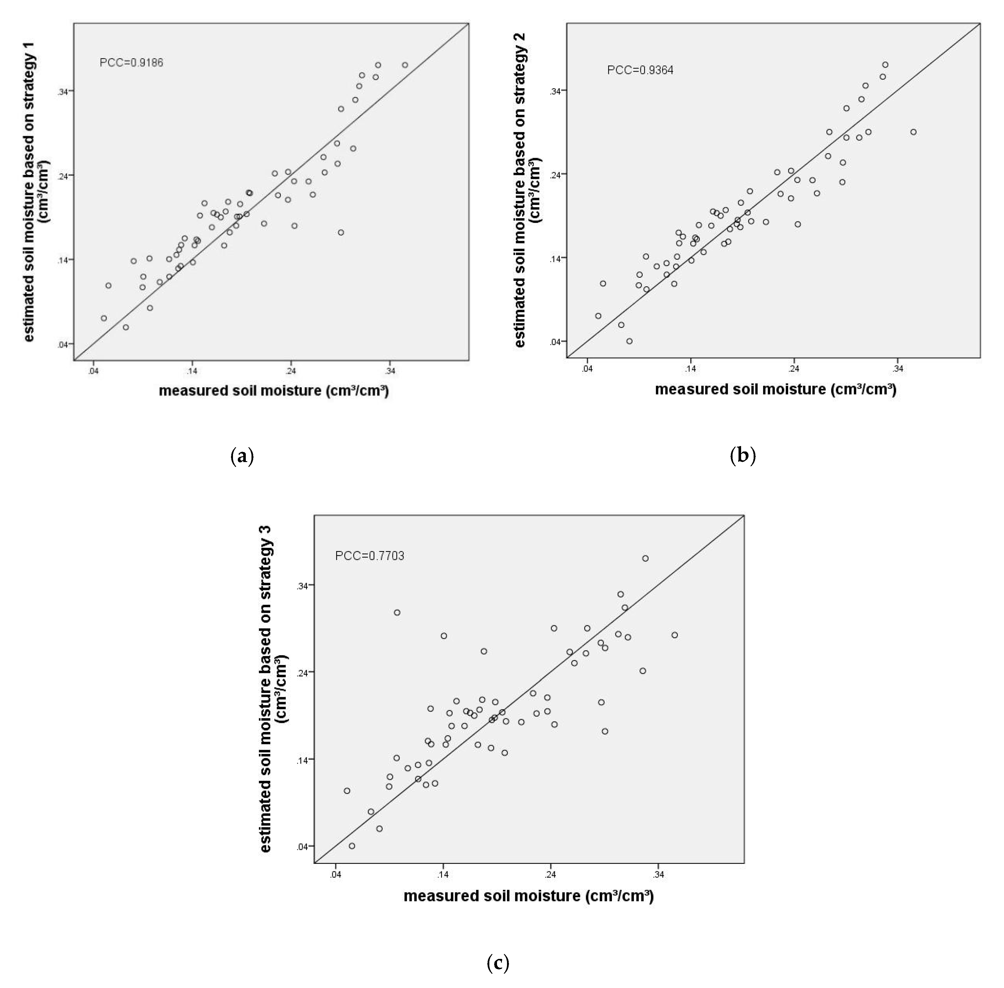
The scatter plot could directly reflect the correlation between the estimated and measured soil moisture values and the corresponding error between them. In this study, a set of scatter plots (Figure 11) were used to show the results of the optimal solution methods under the three different strategies.

Table 9. RMSE, MAE, PCC, and bias between the measured and estimated soil moisture based on the validation dataset.

Modeling Strategies	RMSE (cm³/cm³)	MAE (cm³/cm³)	PCC	BIAS (cm³/cm³)
Strategy 1	0.0314	0.0249	0.9186	−0.0182
Strategy 2	0.0271	0.0225	0.9364	−0.0133
Strategy 3	0.0502	0.0351	0.7703	−0.0231

lists the validation results under the three strategies. The RMSE, MAE, PCC, and bias between the measured soil moisture and the one estimated using the optimal solution method were calculated based on the 60 sample values from the validation dataset acquired during the in-situ measurements. It should be noted that the modeling strategies represent the three strategies for building the optimal solution method, as described in the previous section, based on land use types, percentage content of clay, and slope levels.

In terms of the RMSE and MAE, the soil moisture obtained using the optimal solution method under strategies 2 and 1 was more accurate than that obtained from the nine individual inversion soil moisture maps (the highest precision was: RMSE = 0.0321 cm³/cm³, MAE = 0.0260 cm³/cm³). The optimal solution method under strategy 2 (RMSE = 0.0271 cm³/cm³, MAE = 0.0225 cm³/cm³) exhibited a higher accuracy than the other two models, followed by optimal solution strategy 1 (RMSE = 0.0314 cm³/cm³, MAE = 0.0249 cm³/cm³).

Similarly, the optimal solution method under strategies 2 and 1 exhibited a higher precision than the nine individual inversion soil moisture maps (the highest precision was: PCC = 0.9115 cm³/cm³). As listed in Table 9, the soil moisture estimated using the optimal solution method under strategy 2 had a strong linear relationship, with the PCC value reaching 0.9364. The soil moisture calculated using the optimal solution method under strategy 1 also had a good linear relationship with the measured values (PCC value higher than 0.90).

Interestingly, the bias values of the soil moisture estimated using the optimal solution methods under the three strategies were negative, indicating that all the strategies gave an overall overestimated result.

In this study, a mask file built using the threshold value was used to mask the urban land and water bodies to improve the accuracy of the bare soil moisture estimation. Figure 12 shows the soil moisture map retrieved using the optimal solution method under strategy 2.

In summary, the evaluation and analysis results on the validation dataset are as follows:

(1)

The optimal solution method showed advantages, confirming the assumptions made in this study. Among them, the soil moisture calculated using the optimal solution method under strategies 2 and 1 was more accurate than those obtained from the nine individual inversion soil moisture maps. The RMSE index for the optimal solution method under strategy 2 was 0.005 cm³/cm³ lower than that for the individual estimation model constructed using the AIEM ($m_{v1}$: the only model with the highest accuracy among the nine individual inversion maps), and the RMSE index for the optimal solution method under strategy 1 was 0.0007 cm³/cm³ lower than that for the individual estimation model. Similarly, the PCC index for the optimal solution method under strategy 2 was 0.0249 higher than that for the individual estimation model constructed using the AIEM, and the optimal solution method under strategy 1 was 0.0071 higher than that for the individual estimation model. This means that the error between the estimated results of the optimal solution methods under most strategies and the measured soil moisture was lower and that their linear correlation was stronger compared with the individual inversion models.

(2)

Among the strategies used for constructing the optimal solution methods, strategy 2 gave the best accuracy, followed by strategy 1. Compared with the former two strategies, the accuracy of the optimal solution method under strategy 3 was relatively low. Nevertheless, it was still higher than the accuracy of the nine individual models (77.78%), thus demonstrating its superiority. To some extent, this inconsistent result reflects the sensitivity of the soil moisture to the different background knowledge. For the study area, the optimal solution construction strategy with the clay percentage content as the background knowledge exhibited the best performance, followed by the optimal solution construction strategy with the land use type as the background knowledge. The optimal solution strategy with the slope level as the background knowledge exhibited the lowest performance.

5. Conclusions

To accurately map the soil moisture of a study area in Jiangsu Province, China, in this study, we used both optical and radar remote sensing data in a combined manner, improved and coupled several commonly used inversion models, fully utilized in situ ground experimental datasets, and introduced background knowledge into the optimal solution method.

For study areas with a complex coverage, it is important to effectively remove the influence of vegetation canopy. In the process of removing the influence of vegetation canopy, we made two improvements based on the conventional WCM. A combined VWC model was proposed, and its accuracy (PCC = 0.9442) was found to be significantly higher than that of the one-variable quadratic models. The empirical parameters A, B, and α calculated based on the in situ experimental datasets (WCM_3) were selected as the WCM parameters to remove the effect of vegetation canopy.

Based on an individual inversion algorithm constructed using four commonly used models, nine soil moisture inversion maps were obtained. The estimated model constructed using the AIEM ($m_{v1}$) exhibited a higher accuracy than the other models, followed by the Oh model ($m_{v5}$) and LUT inversion method under HH polarization ($m_{v2}$). In general, the indirect Dubois model ($m_{v6}$, $m_{v7}$, $m_{v8}$, and $m_{v9}$) exhibited a relatively lower inversion accuracy than the direct inversion models ($m_{v1}$, $m_{v2}$, $m_{v3}$, $m_{v4}$, and $m_{v5}$). The possible reasons for these were analyzed. The influencing factors may have included the inherent characteristics of these models, the sensitivity of the radar polarization mode to the soil moisture, and the error transmission of the intermediate parameters of the indirect models.

Notably, we attempted to retrieve the RMS height based on the LUT method; this is a relatively new approach. The RMS height was retrieved from the LUT method and Oh model as input to estimate the soil moisture using the Dubois model. Although the accuracy of these indirect algorithms was relatively lower than that of the direct inversion algorithm, the attempts made gave feasible and valuable results to some extent.

Optimal solution methods were proposed by analyzing the nine individual inversion algorithms with background knowledge. The superiority of the optimal solution method was significant. The model under strategy 2 (RMSE = 0.0271 cm³/cm³, MAE = 0.0225 cm³/cm³, PCC = 0.9364) gave the best accuracy, followed by strategy 1. Compared with the former two strategies, the accuracy of the optimal solution method under strategy 3 was relatively low, though it was still higher than the accuracy of the nine individual models (77.78%). The superiority of the optimal solution methods was attributed to the integration of various categories of the nine individual algorithms with the best accuracy based on background knowledge.

In this study, various efforts were made to retrieve the soil moisture with high accuracy. Some of the individual inversion algorithms and most of the optimal solution methods gave satisfactory results. However, as with any study, there remain some shortcomings: (1) The surface coverage of the study area was complex and inconsistent with the basic assumptions of the WCM. (2) Although the influence of vegetation water was reduced as much as possible, the polarization backscattering coefficient is significantly affected by the structure of the vegetation canopy, which would introduce some errors in the calculation process. (3) There were uncertainties in the in situ measurement of the RMS height, which may have caused errors in the inversion processes. (4) Only a few types of background knowledge data were used in the optimal solution methods, and the construction methods were relatively simple. Future research can be carried out from the following aspects: GF-1 could be replaced by GF-6 to obtain more spectral information; this may give a better accuracy in removing the influence of the vegetation canopy. In the process of bare soil moisture inversion, more diversified and comprehensive multi-model coupling methods could be tried to explore the potential of each model and improve the coupling algorithms. More diverse and representative background knowledge could be introduced in the process of constructing the optimal solution method, and the algorithm used for the construction process can be further improved.

References

1. Anagnostopoulos, V.; Petropoulos, G.P.; Ireland, G.; Carlson, T.N. A modernized version of a 1D soil vegetation atmosphere transfer model for improving its future use in land surface interactions studies. Environ. Model. Softw. 2017, 90, 147–156. [Google Scholar] [CrossRef] [Green Version]
2. Gherboudj, I.; Magagi, R.; Berg, A.A.; Toth, B. Soil moisture retrieval over agricultural fields from multi-polarized and multi-angular RADARSAT-2 SAR data. Remote Sens. Environ. 2011, 115, 33–43. [Google Scholar] [CrossRef]
3. She, D.; Liu, D.; Liu, Y.; Liu, Y.; Xu, C.; Qu, X.; Chen, F. Profile characteristics of temporal stability of soil water storage in two land uses. Arab. J. Geosci. 2014, 7, 21–34. [Google Scholar]
4. Taibi, A.E.O.; Elfeki, A.; Zhang, G. Modeling hydrologic responses of the Zwalm catchment using the REW approach: Propagation of uncertainty in soil properties to model output. Arab. J. Geosci. 2011, 4, 1005–1018. [Google Scholar] [CrossRef]
5. Kornelsen, K.C.; Coulibaly, P. Advances in soil moisture retrieval from synthetic aperture radar and hydrological application. J. Hydrol. 2013, 476, 460–489. [Google Scholar] [CrossRef]
6. Seneviratne, S.I.; Corti, T.; Davin, E.L.; Hirschi, M.; Jaeger, E.B.; Lehner, I.; Orlowsky, B.; Teuling, A.J. Investigating soil moisture–climate interactions in a changing climate: A review. Earth Sci. Rev. 2010, 99, 125–161. [Google Scholar] [CrossRef]
7. Fisher, J.B.; Melton, F.; Middleton, E.; Hain, C.; Anderson, M.; Allen, R.; McCabe, M.F.; Hook, S.; Baldocchi, D.; Townsend, P.A.; et al. The future of evapotranspiration: Global requirements for ecosystem functioning, carbon and climate feedbacks, agricultural management, and water resources. Water Resour. Res. 2017, 53, 2618–2626. [Google Scholar] [CrossRef]
8. Qiaozhen, M.U.; Zhao, M.; Steven, W.J. Improvements to a MODIS global terrestrial evapotranspiration algorithm. Remote Sens. Environ. 2011, 115, 1781–1800. [Google Scholar]
9. Kong, J.; Yang, J.; Zhen, P.; Li, J.; Yang, L. A Coupling Model for Soil Moisture Retrieval in Sparse Vegetation Covered Areas Based on Microwave and Optical Remote Sensing Data. IEEE Trans. Geosci. Remote Sens. 2018, 56, 7162–7173. [Google Scholar] [CrossRef]
10. Amazirh, A.; Merlin, O.; Er-Raki, S.; Gao, Q.; Rivalland, V.; Malbeteau, Y.; Khabba, S.; JoséEscorihuelac, M. Retrieving surface soil moisture at high spatio-temporal resolution from a synergy between Sentinel-1 radar and Landsat thermal data: A study case over bare soil. Remote Sens. Environ. 2018, 211, 321–337. [Google Scholar] [CrossRef]
11. Du, Y.; Ulaby, F.T.; Dobson, M.C. Sensitivity to soil moisture by active and passive microwave sensors. IEEE Trans. Geosci. Remote Sens. 2000, 38, 105–114. [Google Scholar] [CrossRef]
12. Bruckler, L.; Witono, H.; Stengel, P. Near surface soil moisture estimation from microwave measurements. Remote Sens. Environ. 1988, 26, 101–121. [Google Scholar] [CrossRef]
13. Bao, Y.; Zhang, Y.; Wang, J.; Min, J. Surface soil moisture estimation over dense crop using Envisat ASAR and Landsat TM imagery: An approach. Int. J. Remote Sens. 2014, 35, 6190–6212. [Google Scholar] [CrossRef]
14. Baghdadi, N.; Hajj, M.E.; Zribi, M. Coupling SAR C-band and optical data for soil moisture and leaf area index retrieval over irrigated grasslands. IEEE J. Sel. Top. Appl. Earth Obs. Remote Sens. 2016, 9, 3551–3554. [Google Scholar] [CrossRef] [Green Version]
15. Dianjun, Z.; Guoqing, Z. Estimation of Soil Moisture from Optical and Thermal Remote Sensing: A Review. Sensors 2016, 16, 1308. [Google Scholar]
16. Verstraeten, W.W.; Veroustraete, F.; van der Sande, C.J.; Grootaers, I.; Feyen, J. Soil moisture retrieval using thermal inertia, determined with visible and thermal spaceborne data, validated for European forests. Remote Sens. Environ. 2006, 101, 299–314. [Google Scholar] [CrossRef]
17. Yansong, B.; Libin, L.; Shanyu, W.; Deng, K.A.K.; Petropoulos, G.P. Surface soil moisture retrievals over partially vegetated areas from the synergy of Sentinel-1 and Landsat 8 data using a modified water-cloud model. Int. J. Appl. Earth Obs. Geoinf. 2018, 72, 76–85. [Google Scholar]
18. Zhang, X.; Chen, B.; Fan, H.; Huang, J. The Potential Use of Multi-Band SAR Data for Soil Moisture Retrieval over Bare Agricultural Areas: Hebei, China. Remote Sens. 2015, 8, 7. [Google Scholar] [CrossRef] [Green Version]
19. Mattar, C.; Wigneron, J.P.; Sobrino, J.A.; Novello, N.; Calvet, J.C.; Albergel, C.; Richaume, P.; Mialon, A.; Guyon, D.; Jiménez-Muñoz, J.C. A Combined Optical-Microwave Method to Retrieve Soil Moisture Over Vegetated Areas. IEEE Trans. Geosci. Remote Sens. 2012, 50, 1404–1413. [Google Scholar] [CrossRef]
20. Santamaria-Artigas, A.; Mattar, C.; Wigneron, J.P. Application of a Combined Optical-Passive Microwave Method to Retrieve Soil Moisture at Regional Scale Over Chile. IEEE J. Sel. Top. Appl. Earth Obs. Remote Sens. 2016, 9, 1493–1504. [Google Scholar] [CrossRef]
21. Miernecki, M.; Wigneron, J.P.; Lopez-Baeza, E.; Kerr, Y.; De Jeu, R.; De Lannoy, G.J.M.; Jackson, T.J.; O’Neill, P.E.; Schwankh, M.; Moran, R.F.; et al. Comparison of SMOS and SMAP soil moisture retrieval approaches using tower-based radiometer data over a vineyard field. Remote Sens. Environ. 2014, 154, 89–101. [Google Scholar] [CrossRef] [Green Version]
22. Yan, F.; Qin, Z.; Li, M.; Li, W. Progress in soil moisture estimation from remote sensing data for agricultural drought monitoring. Proc. SPIE Int. Soc. Opt. Eng. 2006, 6366, 636601. [Google Scholar]
23. Zeng, J.; Li, Z.; Chen, Q.; Bi, H. Method for Soil Moisture and Surface Temperature Estimation in the Tibetan Plateau Using Spaceborne Radiometer Observations. IEEE Geosci. Remote Sens. Lett. 2015, 12, 97–101. [Google Scholar] [CrossRef]
24. Chen, Q.; Zeng, J.; Cui, C.; Li, Z.; Chen, K.; Bai, X.; Xu, J. Soil Moisture Retrieval From SMAP: A Validation and Error Analysis Study Using Ground-Based Observations Over the Little Washita Watershed. IEEE Trans. Geosci. Remote Sens. 2018, 56, 1394–1408. [Google Scholar] [CrossRef]
25. Ulaby, F.T.; Batlivala, P.P.; Dobson, M.C. Microwave Backscatter Dependence on Surface Roughness, Soil Moisture, and Soil Texture: Part I-Bare Soil. IEEE Trans. Geosci. Electron. 1978, GE-16, 286–295. [Google Scholar] [CrossRef]
26. Zhao, X.; Huang, N.; Song, X.F.; Niu, Z.; Li, Z.Y. A new method for soil moisture inversion in vegetation-covered area based on Radarsat 2 and Landsat 8. J. Infrared Millim. Waves 2016, 35, 609–616. [Google Scholar]
27. Lievens, H.; Verhoest, N.E.C. On the Retrieval of Soil Moisture in Wheat Fields from L-Band SAR Based on Water Cloud Modeling, the IEM, and Effective Roughness Parameters. IEEE Geosci. Remote Sens. Lett. 2011, 8, 740–744. [Google Scholar] [CrossRef]
28. Wang, C.; Qi, J.; Moran, S.; Marsett, R. Soil moisture estimation in a semiarid rangeland using ERS-2 and TM imagery. Remote Sens. Environ. 2004, 90, 178–189. [Google Scholar] [CrossRef]
29. Holah, N.; Baghdadi, N.; Zribi, M.; Bruand, A.; King, C. Potential of ASAR/ENVISAT for the characterization of soil surface parameters over bare agricultural fields. Remote Sens. Environ. 2005, 96, 78–86. [Google Scholar] [CrossRef] [Green Version]
30. Joseph, A.T.; Velde, R.V.D.; O’Neill, P.E.; Lang, R.; Gish, T. Effects of corn on C- and L-band radar backscatter: A correction method for soil moisture retrieval. Remote Sens. Environ. 2010, 114, 2417–2430. [Google Scholar] [CrossRef]
31. Attema, E.P.W.; Ulaby, F.T. Vegetation modeled as a water cloud. Radio Sci. 1978, 13, 357–364. [Google Scholar] [CrossRef]
32. Ulaby, F.T.; Mcdonald, K.; Sarabandi, K.; Dobson, M.C. Michigan microwave canopy scattering model. Int. J. Remote Sens. 1990, 11, 1223–1253. [Google Scholar] [CrossRef]
33. Hu, D.; Guo, N.; Sha, S.; Wang, L. Soil Moisture Retrieved Using Radarsat-2/SAR and MODIS Remote Sensing Data in Vegetated Areas of Loess Plateau Soil Moisture Retrieved Using Radarsat-2/SAR and MODIS Remote Sensing Data in Vegetated Areas of Loess Plateau. Remote Sens. Technol. Appl. 2015, 30. [Google Scholar]
34. Baghdadi, N.; King, C.; Chanzy, A.; Wigneron, J.P. An empirical calibration of the integral equation model based on SAR data, soil moisture and surface roughness measurement over bare soils. Int. J. Remote Sens. 2002, 23, 4325–4340. [Google Scholar] [CrossRef]
35. He, B.; Xing, M.; Bai, X. A Synergistic Methodology for Soil Moisture Estimation in an Alpine Prairie Using Radar and Optical Satellite Data. Remote Sens. 2014, 6, 10966–10985. [Google Scholar] [CrossRef] [Green Version]
36. Fung, A.K.; Li, Z.; Chen, K.S. Backscattering from a randomly rough dielectric surface. IEEE Trans. Geosci. Remote Sens. 1992, 30, 369. [Google Scholar] [CrossRef]
37. Baghdadi, N.; Zribi, M. Evaluation of radar backscatter models IEM, OH and Dubois using experimental observations. Int. J. Remote Sens. 2006, 27, 3831–3852. [Google Scholar] [CrossRef]
38. Wu, T.D.; Chen, K.S.; Fung, A.K.; Tsay, M.K. A transition model for the reflection coefficient in surface scattering. IEEE Trans. Geosci. Remote Sens. 2001, 39, 2040–2050. [Google Scholar]
39. Oh, Y.; Sarabandi, K.; Ulaby, F.T. Semi-empirical model of the ensemble-averaged differential Mueller matrix for microwave backscattering from bare soil surfaces. IEEE Trans. Geosci. Remote Sens. 2002, 40, 1348–1355. [Google Scholar] [CrossRef] [Green Version]
40. Dubois, P.C.; Van Zyl, J.; Engman, T. Measuring soil moisture with imaging radars. IEEE Trans. Geosci. Remote Sens. 1995, 33, 926. [Google Scholar] [CrossRef] [Green Version]
41. Khabazan, S.; Motagh, M.; Hosseini, M. Evaluation of Radar Backscattering Models IEM, OH, and Dubois using L and C-Bands SAR Data over different vegetation canopy covers and soil depths. ISPRS Int. Arch. Photogramm. Remote Sens. Spat. Inf. Sci. 2013, XL-1/W3, 225–230. [Google Scholar] [CrossRef] [Green Version]
42. Huang, S.; Ding, J.; Zou, J.; Liu, B.; Zhang, J.; Chen, W. Soil Moisture Retrival Based on Sentinel-1 Imagery under Sparse Vegetation Coverage. Sensors 2019, 19, 589. [Google Scholar] [CrossRef] [Green Version]
43. Biftu, G.F.; Gan, T.Y. Retrieving near-surface soil moisture from Radarsat SAR data. Water Resour. Res. 1999, 35, 1569–1579. [Google Scholar] [CrossRef]
44. Chai, X.; Zhang, T.; Shao, Y.; Gong, H.; Liu, L.; Xie, K. Modeling and Mapping Soil Moisture of Plateau Pasture Using RADARSAT-2 Imagery. Remote Sens. 2015, 7, 1279–1299. [Google Scholar] [CrossRef] [Green Version]
45. Chiara, P.; Brian, B.; Alexander, G.; Dwyer, E. Quality Assessment of the CCI ECV Soil Moisture Product Using ENVISAT ASAR Wide Swath Data over Spain, Ireland and Finland. Remote Sens. 2015, 7, 15388–15423. [Google Scholar]
46. Dabrowska, K.; Budzynska, M.; Tomaszewska, M.; Malińska, A.; Gatkowska, M.; Bartold, M.; Malek, I. Assessment of Carbon Flux and Soil Moisture in Wetlands Applying Sentinel-1 Data. Remote Sens. 2016, 8, 756. [Google Scholar] [CrossRef] [Green Version]
47. Alexakis, D.D.; Mexis, F.K.; Vozinaki, A.K.; Daliakopoulos, I.N.; Tsanis, I.K. Soil Moisture Content Estimation Based on Sentinel-1 and Auxiliary Earth Observation Products. A Hydrological Approach. Sensors 2017, 17, 1455. [Google Scholar] [CrossRef] [PubMed] [Green Version]
48. Gao, Q.; Zribi, M.; Escorihuela, M.J.; Baghdadi, N. Synergetic Use of Sentinel-1 and Sentinel-2 Data for Soil Moisture Mapping at 100 m Resolution. Sensors 2017, 17, 1966. [Google Scholar] [CrossRef] [Green Version]
49. Rahman, M.S.; Di, L.; Yu, E.; Lin, L.; Zhang, C.; Tang, J. Rapid Flood Progress Monitoring in Cropland with NASA SMAP. Remote Sens. 2019, 11, 191. [Google Scholar] [CrossRef] [Green Version]
50. Meyer, T.; Weihermüller, L.; Vereecken, H.; Jonard, F. Vegetation Optical Depth and Soil Moisture Retrieved from L-Band Radiometry over the Growth Cycle of a Winter Wheat. Remote Sens. 2018, 10, 1637. [Google Scholar] [CrossRef] [Green Version]
51. Wang, C.; Zhang, Z.; Paloscia, S.; Zhang, H.; Wu, F.; Wu, Q. Permafrost Soil Moisture Monitoring Using Multi-Temporal TerraSAR-X Data in Beiluhe of Northern Tibet, China. Remote Sens. 2018, 10, 1577. [Google Scholar] [CrossRef] [Green Version]
52. Leconte, R.; Brissette, F.; Galarneau, M.; Rousselle, J. Mapping near-surface soil moisture with RADARSAT-1 synthetic aperture radar data. Water Resour. Res. 2004, 40. [Google Scholar] [CrossRef]
53. Zhang, L.; Lv, X.; Chen, Q.; Sun, G.; Yao, J. Estimation of Surface Soil Moisture during Corn Growth Stage from SAR and Optical Data Using a Combined Scattering Model. Remote Sens. 2020, 12, 1844. [Google Scholar] [CrossRef]
54. Hoskera, A.K.; Nico, G.; Ahmed, M.I.; Whitbread, A. Accuracies of Soil Moisture Estimations Using a Semi-Empirical Model Over Bare Soil Agricultural Croplands from Sentinel-1 SAR Data. Remote Sens. 2020, 12, 1664. [Google Scholar] [CrossRef]
55. Page, M.L.; Jarlan, L.; El Hajj, M.M.; Zribi, M.; Baghdadi, N.; Boone, A. Potential for the Detection of Irrigation Events on Maize Plots Using Sentinel-1 Soil Moisture Products. Remote Sens. 2020, 12, 1621. [Google Scholar] [CrossRef]
56. Zhang, L.; Meng, Q.Y.; Yao, S.; Wang, Q.; Zeng, J.; Zhao, S.; Ma, J. Soil Moisture Retrieval from the Chinese GF-3 Satellite and Optical Data over Agricultural Fields. Sensors 2018, 18, 2675. [Google Scholar] [CrossRef] [Green Version]
57. He, L.; Chen, J.M.; Chen, K.S. Simulation and SMAP Observation of Sun-Glint Over the Land Surface at the L-Band. IEEE Trans. Geosci. Remote Sens. 2017, 55, 2589–2604. [Google Scholar] [CrossRef]
58. Zribi, M.; Gorrab, A.; Baghdadi, N.; Lili-Chabaane, Z. Influence of Radar Frequency on the Relationship between Bare Surface Soil Moisture Vertical Profile and Radar Backscatter. IEEE Geosci. Remote Sens. Lett. 2014, 848–852. [Google Scholar] [CrossRef] [Green Version]
59. Gong, P.; Wang, J.; Yu, L.; Zhao, Y.; Zhao, Y.; Liang, L. Finer resolution observation and monitoring of global land cover: First mapping results with Landsat TM and ETM+ data. Int. J. Remote Sens. 2013, 34, 2607–2654. [Google Scholar] [CrossRef] [Green Version]
60. Bindlish, R.; Barros, A.P. Parameterization of vegetation backscatter in radar-based, soil moisture estimation. Remote Sens. Environ. 2001, 76, 130–137. [Google Scholar] [CrossRef]
61. Hansan, Z.; Quan, J. Accurate Measurement of Key Parameters of Film Capacitors for EV Power Control Unit. In Proceedings of the 2019 IEEE 4th Int. Future Energy Electronics Conference (IFEEC), Singapore, 25–28 November 2019; Volume 10, p. 1109. [Google Scholar]
62. Eom, H.J.; Fung, A.K. A scatter model for vegetation up to Ku-band. Remote Sens. Environ. 1984, 15, 185–200. [Google Scholar] [CrossRef]
63. Zhang, J.H.; Xu, Y.; Yao, F.M.; Wng, P.J.; Gou, W.J.; Yang, L.M. Advances in estimation methods of vegetation water content based on optical remote sensing techniques. Sci. China Technol. Sci. 2010, 5, 5–13. [Google Scholar] [CrossRef]
64. Prakash, R.; Singh, D.; Pathak, N.P.A. Fusion approach to retrieve soil moisture with SAR and optical data. Remote Sens. 2012, 5, 196–206. [Google Scholar] [CrossRef]
65. Bai, X.; He, B.; Li, X. Optimum Surface Roughness to Parameterize Advanced Integral Equation Model for Soil Moisture Retrieval in Prairie Area Using Radarsat-2 Data. IEEE Trans. Geosci. Remote Sens. 2016, 54, 2437–2449. [Google Scholar] [CrossRef]
66. Zheng, X.M.; Ding, Y.L.; Zhao, K.; Jiang, T.; Li, X.F.; Zhang, S.Y.; Li, Y.Y.; Wu, L.L.; Sun, J.; Ren, J.H.; et al. Estimation of Vegetation Water Content from Landsat 8 OLI Data. Spectrosc. Spectr. Anal. 2014, 34, 3385–3390. [Google Scholar]
67. Zeng, J.; Chen, K.S.; Liu, Y.; Bi, H.; Chen, Q. Radar Response of Off-Specular Bistatic Scattering to Soil Moisture and Surface Roughness at L-Band. IEEE Geosci. Remote Sens. Lett. 2016, 13, 1–5. [Google Scholar] [CrossRef]
68. Dobson, M.C. Microwave dielectric behavior of wet soil-Part II: Dielectric-mixing models. IEEE Trans. Geosci. Remote Sens 1985, 23, 35–46. [Google Scholar] [CrossRef]
69. Barber, M.; Grings, F.; Perna, P.; Piscitelli, M.; Maas, M.; Bruscantini, C.A.; Jacobo-berlles, J.; Karszenbaum, H. Speckle Noise and Soil Heterogeneities as Error Sources in a Bayesian Soil Moisture Retrieval Scheme for SAR Data. IEEE J. Sel. Top. Appl. Earth Obs. Remote Sens. 2012, 5, 942–951. [Google Scholar] [CrossRef]
70. Zribi, M.; Dechambre, M. A new empirical model to retrieve soil moisture and roughness from C-band radar data. Remote Sens. Environ. 2003, 84, 42–52. [Google Scholar] [CrossRef]
71. Shi, J.; Wang, J.; Hsu, A.Y.; O’Neill, P.E.; Engman, E.T. Estimation of bare surface soil moisture and surface roughness parameter using L-band SAR image data. IEEE Trans. Geosci. Remote Sens. 2002, 35, 1254–1266. [Google Scholar]
72. Chen, J.; Jia, Y.; Yu, F. Soil moisture inversion by radar with dual-polarization. Trans. Chin. Soc. Agric. Eng. 2013, 5, 109–115. [Google Scholar]
73. Gou, S.; Bai, X.; Chen, Y.; Zhang, S.; Zhu, Q.; Du, P. An Improved Approach for Soil Moisture Estimation in Gully Fields of the Loess Plateau Using Sentinel-1A Radar Images. Remote Sens. 2019, 11, 349. [Google Scholar]
74. Brunner, D.; Bruzzone, L.; Ferro, A.; Fortuny, J.; Lemoine, G. Analysis of the double bounce scattering mechanism of buildings in VHR SAR data. Proc. SPIE Int. Soc. Opt. Eng. 2008, 7109. [Google Scholar] [CrossRef]
75. Al-Bakri, J.; Suleiman, A.; Berg, A. A comparison of two models to predict soil moisture from remote sensing data of RADARSAT II. Arab. J. Geosci. 2014, 7, 4851–4860. [Google Scholar] [CrossRef]
Figure 1. (a) Geographical location of the study area and (b) major land-cover types.
Remotesensing 12 02123 g001
Figure 2. Map of sampling sites and elevation (a) and statistical characteristics of measured soil moisture samples (b).
Remotesensing 12 02123 g002
Figure 3. Calibration of volumetric soil moisture acquired by TDR probes.
Remotesensing 12 02123 g003
Figure 4. Flowchart of the proposed soil moisture mapping. VWC, vegetation water content; mvn, soil moisture content obtained by four commonly used models; s and l: the root-mean-square (RMS) height and correlation length.
Remotesensing 12 02123 g004
Figure 5. Schematic of the optimal solution method based on a specific background knowledge. Color: pixel classification results; Pattern: soil moisture results after mosaic.
Remotesensing 12 02123 g005
Figure 6. Scatter plot between the measured and estimated vegetation water content values using the new empirical model based on 19 sample datasets. The 1:1 line is included in the plot.
Remotesensing 12 02123 g006
Figure 7. Scatter plots between the bare soil backscattering (dB) simulated by AIEM and three different water-cloud model strategies based on experimental data. The 1:1 line is included in the plot. (a) WCM_1; (b) WCM_2; (c) WCM_3.
Remotesensing 12 02123 g007
Figure 8. Responses of the soil moisture and soil backscattering coefficient: (a,c) HH polarization; (b,d) VV polarization.
Remotesensing 12 02123 g008aRemotesensing 12 02123 g008b
Figure 9. Responses of the roughness parameters and soil backscattering coefficient: (a,c) HH polarization; (b,d) VV polarization.
Remotesensing 12 02123 g009aRemotesensing 12 02123 g009b
Figure 10. Responses of soil moisture and soil backscattering coefficients. (a) HH polarization; (b) VV polarization.
Remotesensing 12 02123 g010
Figure 11. Scatter plots between the measured and estimated soil moisture values obtained using the optimal solution methods based on the 60 in situ experimental datasets. A 1:1 line is included in this plot. (a) strategy 1; (b) strategy 2; (c) strategy 3.
Remotesensing 12 02123 g011
Figure 12. Map of retrieved soil moisture content based on the optimal solution method under strategy 2.
Remotesensing 12 02123 g012