Geosynchronous Spaceborne-Airborne Bistatic Moving Target Indication System: Performance Analysis and Configuration Design

Abstract

Geosynchronous spaceborne-airborne bistatic synthetic aperture radar (GEO SA-BSAR), consisting of GEO transmitter and airborne receiver, has stable coverage for a long time and benefits moving target detection. However, the performance of GEO SA-BSAR moving target indication (MTI) system varies widely between bistatic configurations. The traditional configuration design for GEO SA-BSAR system only considers the imaging performance, which may cause the poor MTI performance. In this paper, we propose a bistatic configuration design method to jointly optimize the MTI and SAR imaging performance for GEO SA-BSAR MTI system. The relationship between the MTI performance and bistatic configuration parameters is derived analytically and analyzed based on the maximum output signal to clutter and noise ratio (SCNR) criterion. Then, the MTI performance and SAR imaging performance are jointly considered to model the configuration design problem as a multi-objective optimization problem under the constrained condition. Finally, the optimal configuration for GEO SA-BSAR MTI system is given.

1. Introduction

Bistatic synthetic aperture radar (BSAR), whose transmitter and receiver are located on different platforms, has attracted much attention in recent years. BSAR has advantages of stealthy and flexible configuration, which can help it to detect and monitor moving targets in the complex electromagnetic environment. In particular, for the BSAR system with existing spaceborne transmitter and airborne receiver, only the receiving equipment is needed to be deployed that significantly reduces the cost and the spaceborne SAR with high orbit can provide a wide monitoring scope. Several successful experiments on spaceborne-airborne BSAR (SA-BSAR) had been carried out by NASA’s Jet Propulsion Laboratory (JPL) in 1984 [1] and by the German Aerospace Center (DLR) and the Research Establishment for Applied Science (FGAN) from 2007 to 2009 [2,3,4,5,6,7], respectively. These experiments constrained the satellite and the airplane to fly along parallel flight paths and achieved the stationary scenes imaging. This means that the basic and core problems for SA-BSAR system can be solved, such as the beam, time and phase synchronization [2,8], platform motion compensation [3], imaging algorithm [4,5,6,7], etc. It is also indicated that we can take the advantages of SA-BSAR system to apply it to the moving target indication (MTI).

Low earth orbit SA-BSAR (LEO SA-BSAR) system, whose major mission is for stationary scenes imaging, is hard to measure slow velocity for its clutter spectrum broadening seriously. However, with the significant increase of transmitter’s orbital altitude, the ground speed of geosynchronous SA-BSAR (GEO SA-BSAR) reduces [9]. Thus, it can provide stable coverage area or a long time for airborne receiver. In addition, GEO SA-BSAR also has the advantages of larger coverage and shorter revisit time compared with LEO SAR case [10,11], which benefits MTI. At present, the research on GEO SAR has attracted much attention and involves in all aspects, including system design and optimization [12,13,14], resolution analysis [15,16], accurate imaging algorithm [17,18], deformation retrieval [19] and MTI [20,21,22], which prompts the development of GEO SA-BSAR MTI system.

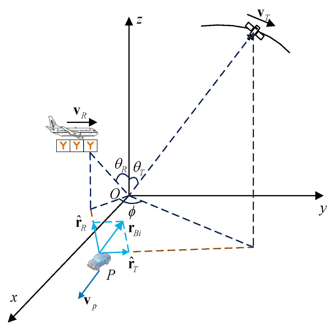
In order to monitor moving target in a particular area, GEO SA-BSAR MTI system determines the system operating time according to the ephemeris, attitude and antenna beam direction of GEO SAR to ensure the area can always be illuminated during the synthetic aperture time. Then, the airborne multi-channel receiver can obtain and process the echoes to detect the moving targets. Considering the beam of GEO SAR covers thousands of kilometers and the airplane’s flight path can be designed in advance, the configuration of GEO SA-BSAR MTI system is flexible, leading to different MTI performance.

As early as 1997, the system with geosynchronous illumination and bistatic reception was first proposed for large coverage monitoring and MTI [23]. It only analyzed the feasibility of MTI based on the system parameters without considering the configuration design and data processing. Subsequently, the research of GEO SA-BSAR focuses on imaging characteristics, resolution, bistatic configuration and imaging algorithm for stationary scenes [24,25,26,27,28,29,30]. Literature [26] analyzed the imaging performance of GEO SA-BSAR system under different bistatic configuration, based on which the bistatic configuration for GEO SA-BSAR imaging system was obtained to make the imaging performance indicators approach to the given values as far as possible. However, the configuration for MTI is not considered, causing the poor MTI performance if the configuration for imaging stationary scenes is employed directly.

In addition, the research on GEO SA-BSAR MTI system mainly focuses on the geostationary SA-BSAR. The MTI processing of geostationary SA-BSAR has been studied in literature [31], in which two airborne side-looking radars with different carrier frequencies, antenna spacings or velocities were adopted to solve the azimuth ambiguity problem. However, there are few studies on non-geostationary SA-BSAR MTI system.

Without changing the equipment, good MTI performance and SAR imaging performance can be achieved at the same time only by changing the bistatic configuration. The key to determine the system configuration is to obtain the relationship between the performance indicators and configuration parameters, which was not involved in previous studies. Then, the configuration design problem is modeled as an optimization problem of MTI performance and SAR imaging performance. Therefore, this paper proposes a configuration design method of GEO SA-BSAR MTI system to achieve the optimal MTI performance while ensuring good SAR imaging performance. The main contributions of this paper are twofold. First, the relationship between the MTI performance and bistatic configuration parameters has been analyzed theoretically. Second, it obtain the bistatic configuration that ensures GEO SA-BSAR system has the best performance of MTI while imaging stationary scene, which extends the function of GEO SA-BSAR system. This has been added in the text.

In this paper, the observation geometry and special issues of the bistatic configuration for GEO SA-BSAR MTI system are introduced in Section 2. Next, in Section 3, the performance of GEO SA-BSAR MTI system is first investigated under the arbitrary bistatic configuration. The performance indicator of MTI system includes signal to clutter and noise ratio (SCNR) loss and Cramer–Rao lower bounds (CRLB). Based on optimal output SCNR criterion, the analytical expressions of minimum detectable velocity (MDV), the maximum unambiguous velocity (MUV) in terms of configuration parameters can be obtained. Moreover, the theoretical variance of parameter estimation is deduced based on CRLB. Then, according to the relationship between MTI performance and configuration parameters and SAR imaging performance requirements, Section 4 models the configuration design problem as a multi-objective optimization problem containing constraint conditions. Considering the objective functions are more than three, the constraint non-dominated sorting evolutionary algorithm III is used to optimize bistatic configuration and more than one solution can be obtained at the same time. The best bistatic configuration of GEO SA-BSAR MTI system can be selected from the solutions to guide aircraft flight track. In Section 5 the optimal configuration of GEO SA-BSAR MTI system is obtained through simulation, and the performance of the system is also verified by simulation. Finally, the conclusion is given.

2. GEO SA-BSAR System for MTI

2.1. System and Geometry

GEO SA-BSAR MTI system transmits signals by GEO SAR, which can provide a stable beam coverage for a long time. Then, the airplane equipped with a multi-channel receiver obtains the echoes from the surface that can be illumined by GEO SAR. The reference point local coordinate system is selected to analyze the geometric model of GEO SA-BSAR MTI system. The coordinate system has its origin at the center of the interest scene, with the z-axis vertical, the y-axis pointing to the flight direction of airplane and the x-axis completes the right-handed system. The geometric relationship between the GEO SA-BSAR MTI system and the ground target is shown in Figure 1. The airplane flies along the y-axis with the constant speed $v_R$ and the velocity of GEO SAR at the aperture center moment (ACM) is $v_T$. $\psi$ is the ground projection of the velocity angle between $v_R$ and $v_T$. Moreover, the incidence angle of GEO SAR is ${\theta }_T$. The first channel of the airborne multichannel receiver is regarded as reference channel and its incidence angle is ${\theta }_R$. The ground projection of bistatic angle is $\varphi$.

For the ground target $P$ locating at $\left(x_0,y_0\right)$, ${\widehat{r}}_R$ is the ground projection of unit vector of the slant range between the target and airplane at ACM, ${\widehat{r}}_T$ is the ground projection of unit vector of the slant range between the target and GEO satellite at ACM and the sum of ${\widehat{r}}_R$ and ${\widehat{r}}_T$ is $r_{Bi}$. During the synthetic aperture time, the target is assumed to be in uniform motion with the velocity of $v_p={\left(v_x,v_y\right)}^T$. It is a stationary target when $v_p=0$. In addition, the system parameters of GEO SA-BSAR adopted in this paper are shown in

Table 1. Receiver system parameters and GEO SAR orbit elements of GEO SA-BSAR MTI system.

Receiver System Parameters		GEO SAR Orbit Elements
Wavelength	0.24 m	Eccentricity	0
Bandwidth	100 MHz	Inclination	16°
Receiver’s height	10 km	Semi-major axis	42,164 km
Receiver’s velocity	200 m/s	Longitude of ascending node	88°
Synthetic aperture time	10 s
Number of channels	3	Argument of perigee	——
Antenna size	6 m

.

2.2. Bistatic Configuration

With the trajectory of GEO SAR known by ephemeris, the flight track can be determined by $\psi$, ${\theta }_R$ and $\varphi$. Different $\psi$, ${\theta }_R$ and $\varphi$ lead to different SAR imaging performance and MTI performance. The SAR imaging performance is described in this section.

The imaging performance indicators of GEO SA-BSAR imaging system mainly include the ground range resolution ${\rho }_{gr}$, the azimuth resolution ${\rho }_{az}$, the resolution direction angle $\zeta$ and the clutter to noise ratio (CNR) (Since the stationary scene is regarded as the clutter in MTI, the signal to noise ratio (SNR) of the stationary target is as the CNR in this paper). Literature [26,32,33] analyzed the influence of bistatic configuration on imaging performance of static scene in detail:

$$\{\begin{array}{l}{\rho }_{gr}=\frac{0.886c}{B_r\Vert r_{Bi}\Vert }\\ {\rho }_{az}=\frac{0.886\lambda }{{\displaystyle \underset{T_a}{\int }\Vert H^{\perp }\left({\mathsf{\omega }}_{TP}\left(t_a\right)+{\mathsf{\omega }}_{RP}\right)\Vert d{t}_a}}\\ \zeta ={\cos }^{-1}\left(\mathsf{\Theta }\cdot \mathsf{\Xi }\right)\\ CNR=\frac{P_t{G}_t{G}_r{\sigma }_0{\rho }_{gr}{\rho }_{az}{\lambda }^2{T}_a{D}_c}{{\left(4\pi \right)}^3{R}_t^2{R}_r^2{L}_{T}k{T}_0{F}_n}\end{array}$$

(1)

According to the geometric relationship, $\Vert r_{Bi}\Vert$ is determined by bistatic configuration parameters ${\theta }_R$ and $\varphi$. ${\sigma }_0$ is the normalized radar cross section, which can be calculated according to [34].

According to the preset requirements of imaging performance indicators, the genetic algorithm was used to obtain the bistatic configuration to ensure actual performance was closest to the requirements. The genetic algorithm is proposed based on the evolution to solve the optimization problems [35,36]. In this paper, the parameters shown in Table 1 are used to obtain the bistatic configuration that meets ${\rho }_{grD}=3m$, ${\rho }_{azD}=3m$, ${\zeta }_D={90}^{\circ }$ and $CN{R}_D=20 \mathrm{dB}$. The configuration design results are shown in

Table 2. The bistatic configuration of GEO SA-BSAR system for stationary scene imaging.

Bistatic Configuration			Imaging Performance
${\theta }_R$ (°)	$\varphi$ (°)	$\psi$ (°)	${\rho }_{gr}$ (m)	${\rho }_{az}$ (m)	$\alpha$ (°)	$CNR$ (dB)
66.9126	347.8532	194.8475	3.0577	3.0425	89.9844	20.0000

.

2.3. Special Issues for Moving Target Indication

The traditional GEO SA-BSAR bistatic configuration design only optimizes the imaging performance of the stationary scenes. This design scheme does not consider the MTI performance, so the MTI performance may be poor and the moving target cannot even be detected.

For the optimal configuration design results for GEO SA-BSAR stationary scenes imaging in Table 2, the MUV is only 16.55 m/s (the calculation expression can be seen Section 3), which does not benefit moving target detection. Therefore, in order to determining the bistatic configuration of GEO SA-BSAR MTI system, the MTI performance and imaging performance are exploited together to rebuild the multi-objective optimization function to obtain the configuration that is suitable for MTI and meets the conditions of GEO SA-BSAR imaging.

The key to determine the bistatic configuration of GEO SA-BSAR MTI system is to establish the analytical expression between the MTI performance and configuration parameters. The performance of BSAR GMTI is usually characterized by the output SCNR loss curve, which cannot visually represent the relationship between the MTI performance and configuration parameters. Therefore, it is necessary to extract key performance indicators from the output SCNR loss curve and derive their analytical expression about configuration parameters, which is used to guide configuration design.

3. Signal Model and Performance Analysis of GEO SA-BSAR MTI System

The performance indicators to be optimized include the MDV, MUV, location accuracy and velocity accuracy of the GEO SA-BSAR MTI system. In this section, according to the GEO SA-BSAR signal model in range-Doppler domain, the clutter covariance matrix of GEO SA-BSAR is derived and the steering vector of moving target is obtained. Then, the analytical expression of MTI performance indicators is derived.

3.1. Signal Model

3.1.1. Clutter Signal Model and Clutter Covariance Matrix

The clutter of GEO SA-BSAR can be expressed as the superposition of all stationary targets. Based on the GEO SA-BSAR stationary target signal model in literature [29], after the range migration correction and range compression, the signal model of the $m$-th channel can be expressed as:

$$\begin{array}{c}{s}_{c,m}\left(t_r,t_a\right)={\displaystyle \iint \sigma \left(x_0,y_0\right)\sin \mathrm{c}\left[B_r\left(t_r-\frac{R_{bi0}+k_{T1}{y}_m/v_R}{c}\right)\right]{\omega }_{a,c}\left(\frac{t_a}{T_a}\right)}\\ \times \exp \left\{-j\frac{2\pi }{\lambda }\left[R_{bi,m}\left(x_0,y_0;t_a\right)-k_{10}{t}_a\right]\right\}d{x}_{0}d{y}_0\end{array}$$

(2)

where the subscript $c$ represents the clutter. In addition, $\left(x_0,y_0\right)$ represents the position coordinates of the stationary target and $\sigma \left(x_0,y_0\right)$ represents the scattering characteristics of the target.

Considering that SAR STAP processing is carried out in the range-Doppler domain, the signal in the range-Doppler domain of the stationary clutter in the $m$-th channel of GEO SA-BSAR can be obtained by using the series reversal method and the principle of stationary phase [37]:

$$\begin{array}{c}{s}_{c,m}^{rd}\left(t_r,f_a\right)=\exp \left\{j\frac{2\pi }{\lambda }{d}_{c,m}\left(f_a\right)\right\}{\displaystyle \iint \sin \mathrm{c}\left[B_r\left(t_r-\frac{R_{bi0}+k_{T1}{y}_m/v_R}{c}\right)\right]}\\ \times W_{a,c}\left(f_a\right)\sigma \left(x_0,y_0\right)\exp \left\{-j{\psi }_c\left(x_0,y_0;f_a\right)\right\}d{x}_{0}d{y}_0\end{array}$$

(3)

where $\exp \left\{-j{\psi }_t\left(x_0,y_0;f_a\right)\right\}$ represents the same phase term of different channels and $\exp \left\{j\frac{2\pi }{\lambda }{d}_{t,m}\left(x_0,y_0;f_a\right)\right\}$ represents the phase difference term of the $m$-th channel relative to the reference channel:

$$\begin{array}{c}{\psi }_c\left(x_0,y_0;f_a\right)=\frac{2\pi R_{bi0}}{\lambda }-\frac{\pi \lambda }{2k_{bi2}}{\left(f_a+\frac{k_{bi1}-k_{10}}{\lambda }\right)}^2-\frac{\pi {\lambda }^2{k}_{bi3}}{4k_{bi2}^3}{\left(f_a+\frac{k_{bi1}-k_{10}}{\lambda }\right)}^3\\ -\frac{2\pi {\lambda }^3\left(9k_{bi3}^2-4k_{bi2}{k}_{bi4}\right)}{64k_{bi2}^5}{\left(f_a+\frac{k_{bi1}-k_{10}}{\lambda }\right)}^4\end{array}$$

(4)

$$d_{c,m}\left(f_a\right)=-k_{T1}\frac{y_m}{v_R}-\lambda \frac{y_m}{v_R}{f}_a$$

(5)

As a result that the imaging scene of GEO SA-BSAR is very small compared with GEO SAR, the change of $d_{c,m}$ is far less than $\lambda /16$ with the space variant $k_{T1}$, which means the changes of $d_{c,m}$ can be ignored. Therefore, for any range-Doppler cell, there is only a fixed phase difference between the signal model of $m$-th channel and reference. Then, the normalized steering vector of clutter can be expressed as $p_c\left(f_a\right)=\frac{1}{\sqrt{M}}{\left[\begin{array}{cccc}1& \exp \left\{j2\pi d_{c,2}/\lambda \right\}& \cdots & \exp \left\{j2\pi d_{c,M}/\lambda \right\}\end{array}\right]}^T$. The clutter covariance matrix can be written as:

$$R_Q\left(f_a\right)=R_N+R_C={\sigma }_n^2{I}_M+E\left[C\left(f_a\right)C^H\left(f_a\right)\right]$$

(6)

where $R_N$ is the noise covariance matrix. $R_C$ is the covariance matrix of the static scene signal. $C\left(f_a\right)$ is the multi-channel clutter and is expressed as:

$$C\left(f_a\right)={\left[\begin{array}{ccc}{s}_{c,1}^{rd}\left(f_a\right)& \cdots & s_{c,M}^{rd}\left(f_a\right)\end{array}\right]}^T$$

(7)

Suppose the amplitude of clutter obeys the Gaussian distribution with mean value of zero and variance of ${\sigma }_c^2$. Moreover, the different clutter points are independent of each other that means:

$$E\left\{\sigma \left(x_1,y_1\right)\cdot {\sigma }^H\left(x_2,y_2\right)\right\}=0,\left(x_1,y_1\right)\ne \left(x_2,y_2\right)$$

(8)

Then, the cross term of different clutter scatterers in the covariance matrix is zero, and the covariance matrix can be rewritten as:

$$R_Q\left(f_a\right)={\sigma }_n^2{I}_M+{\sigma }_c^2{A}_{a,c}^2\left(f_a\right)p_c\left(f_a\right)p_c^H\left(f_a\right)$$

(9)

where $A_{a,c}^2\left(f_a\right)$ is the term generated by the azimuthal envelope, which can be expressed as:

$$A_{a.c}^2\left(f_a\right)={\displaystyle \iint W_{a,c}^2\left(f_a\right)d{x}_{0}d{y}_0}$$

(10)

According to the matrix inverse lemma, it is obtained that:

$$R_Q^{-1}\left(f_a\right)=\frac{1}{{\sigma }_n^2}\left[I_M-\frac{{\sigma }_c^2{A}_{a,c}^2\left(f_a\right)}{{\sigma }_n^2+M{\sigma }_c^2{A}_{a,c}^2\left(f_a\right)}{p}_c\left(f_a\right)p_c^H\left(f_a\right)\right]$$

(11)

3.1.2. Signal Model of Moving Target in RD Domain and Its Steering Vector

After range compression and range migration correction of the stationary target, the moving target’s signal is transformed to the range-Doppler domain:

$$\begin{array}{c}{s}_{t,m}^{rd}\left(t_r,f_a\right)={\sigma }_t\left(x_0,y_0\right)\sin \mathrm{c}\left[B_r\left(t_r-\frac{R_{bi0}+\Delta R_{bi,t}\left(f_a\right)}{c}\right)\right]W_{a,t}\left(f_a\right)\\ \times \exp \left\{-j{\psi }_t\left(x_0,y_0;f_a\right)\right\}\exp \left\{j\frac{2\pi }{\lambda }{d}_{t,m}\left(x_0,y_0;f_a\right)\right\}\end{array}$$

(12)

where the subscript $t$ represents the moving target.

$$\begin{array}{c}{\psi }_t\left(x_0,y_0;f_a\right)=\frac{2\pi R_{bi0}}{\lambda }-\frac{\pi \lambda }{2k_{bi2,t}}{\left(f_a+\frac{k_{bi1,t}-k_{10}}{\lambda }\right)}^2-\frac{\pi {\lambda }^2{k}_{R3,t}}{4k_{bi2,t}^3}{\left(f_a+\frac{k_{bi1,t}-k_{10}}{\lambda }\right)}^3\\ -\frac{2\pi {\lambda }^3\left(9k_{R3,t}^2-4k_{bi2,t}{k}_{R4,t}\right)}{64k_{bi2,t}^5}{\left(f_a+\frac{k_{bi1,t}-k_{10}}{\lambda }\right)}^4\end{array}$$

(13)

$$\begin{array}{c}{d}_{t,m}\left(x_0,y_0;f_a\right)=-k_{T1,t}\frac{y_m}{v_R}-\lambda \frac{y_m}{v_R}{f}_a+\frac{v_x\left(x_R-x_0\right)+v_y\left(y_R-y_0\right)}{v_R{R}_{R0}}{y}_m\\ =-k_{T1}\frac{y_m}{v_R}-\lambda \frac{y_m}{v_R}{f}_a+\frac{v_r\Vert r_{Bi}\Vert }{v_R}{y}_m\end{array}$$

(14)

The phase difference between different channels is related to the target velocity, where

$$v_r=\frac{v_x}{\Vert r_{Bi}\Vert }\left(\frac{x_R-x_0}{R_{R0}}+\frac{x_{T0}-x_0}{R_{T0}}\right)+\frac{v_y}{\Vert r_{Bi}\Vert }\left(\frac{y_R-y_0}{R_{R0}}+\frac{y_{T0}-y_0}{R_{T0}}\right)$$

(15)

$$\Vert r_{Bi}\Vert =\sqrt{{\left(\frac{x_R-x_0}{R_{R0}}+\frac{x_{T0}-x_0}{R_{T0}}\right)}^2+{\left(\frac{y_R-y_0}{R_{R0}}+\frac{y_{T0}-y_0}{R_{T0}}\right)}^2}$$

(16)

The physical meaning of the velocity $v_r$ is the projection of the target’s velocity in the direction of the vector $r_{Bi}$. Therefore, the normalized steering vector of the moving target is:

$$p_t\left(f_a,{\mathsf{\vartheta }}_s\right)=\frac{1}{\sqrt{M}}{\left[\begin{array}{cccc}1& \exp \left\{j2\pi d_{t,2}/\lambda \right\}& \cdots & \exp \left\{j2\pi d_{t,M}/\lambda \right\}\end{array}\right]}^T$$

(17)

3.2. MTI Performance Analysis of GEO SA-BSAR

3.2.1. Minimum Detectable Velocity

The MDV of GEO SA-BSAR system is related to the loss of the moving target’s output SCNR. It is considered that the target cannot be detected when the output SCNR loss exceeds 5 dB [38], so the MDV is the corresponding velocity when the SCNR loss is equal to 5 dB.

The ISTAP algorithm [39] can be used to obtain the optimal output SCNR of GEO SA-BSAR MTI system. First of all, the multichannel signals after time calibration is transformed to the range-Doppler domain. Then, the clutter suppression and beamforming are achieved by post-Doppler STAP after processing. Finally, the azimuthal pulse compression is used to get the SAR image. The target detection is achieved in SAR images. Under the above algorithm, the filtered signal should be coherently accumulated along the azimuth direction, so the SCNR loss can be expressed as:

$$SCN{R}_{loss}\left({\mathsf{\vartheta }}_s\right)=\frac{SCN{R}_{out}}{SNR}=\frac{{\displaystyle \int S^H\left(f_a,{\mathsf{\vartheta }}_s\right)R_Q^{-1}\left(f_a\right)S\left(f_a,{\mathsf{\vartheta }}_s\right)}d{f}_a}{{\displaystyle \int S^H\left(f_a,{\mathsf{\vartheta }}_s\right)S\left(f_a,{\mathsf{\vartheta }}_s\right)}d{f}_a/{\sigma }_n^2}$$

(18)

where $S\left(f_a,{\mathsf{\vartheta }}_s\right)$ is the multi-channel signal of moving target in range-Doppler domain, which can be represented as:

$$S\left(f_a,{\mathsf{\vartheta }}_s\right)={\left[\begin{array}{ccc}{s}_{t,1}^{rd}\left(f_a\right)& \cdots & s_{t,M}^{rd}\left(f_a\right)\end{array}\right]}^T$$

(19)

Substitute Equations (11) and (19) into Equation (18) to get:

$$SCN{R}_{loss}\left({\mathsf{\vartheta }}_s\right)=\frac{{\sigma }_n^2}{{\sigma }_t^2{\displaystyle \int W_{a,t}^{2}d{f}_a}}{\displaystyle \int \left(\frac{{\sigma }_t^2{W}_{a,t}^2}{{\sigma }_n^2}-\frac{{\sigma }_t^2{W}_{a,t}^2}{{\sigma }_n^2}\cdot \frac{{\sigma }_c^2{A}_{a,c}^2}{{\sigma }_n^2+{\sigma }_c^2{A}_{a,c}^2}{p}_t^H{p}_c{p}_c^H{p}_t\right)d{f}_a}$$

(20)

where

$$\begin{array}{cc}{p}_t^H\left(f_a,{\mathsf{\vartheta }}_s\right)p_c\left(f_a\right)& =\frac{1}{M}{\displaystyle \sum _{m=1}^M\exp \left\{j\frac{2\pi }{\lambda }\left(d_{c,m}-d_{t,m}\right)\right\}}\\ & =\frac{1}{M}{\displaystyle \sum _{m=1}^M\exp \left\{-j\frac{2\pi v_r\Vert r_{Bi}\Vert }{\lambda v_R}{y}_m\right\}}\end{array}$$

(21)

For linear array, $y_m=\left(m-1\right)d$ and it can be calculated that:

$$\begin{array}{cc}SCN{R}_{loss}\left({\mathsf{\vartheta }}_s\right)& =1-\frac{{\sin }^2\left(\pi M\beta \right)}{M^2{\sin }^2\left(\pi \beta \right)}\frac{1}{{\displaystyle \int W_{a,t}^{2}d{f}_a}}{\displaystyle \int \frac{{\sigma }_c^2{A}_{a,c}^2}{{\sigma }_n^2+{\sigma }_c^2{A}_{a,c}^2}{W}_{a,t}^{2}d{f}_a}\hfill \\ & =1-\frac{{\sin }^2\left(\pi M\beta \right)}{{\sin }^2\left(\pi \beta \right)}\frac{{\displaystyle \int CNR\cdot A_{a,c}^2\cdot W_{a,t}^2/\left(1+CNR\cdot A_{a,c}^2\right)d{f}_a}}{M^2{\displaystyle \int W_{a,t}^{2}d{f}_a}}\hfill \end{array}$$

(22)

where $\beta =\frac{d\cdot v_r\Vert r_{Bi}\Vert }{\lambda v_R}$. The expression of the output SCNR loss can be used to derive the MDV of the moving target. It is considered that when the SNR loss is $-X\mathrm{dB}$, the corresponding speed is the MDV. It is satisfied that:

$$\frac{\sin c\left(M\beta \right)}{\sin c\left(\beta \right)}\approx \frac{M^2{\displaystyle \int W_{a,t}^{2}d{f}_a}}{{\displaystyle \int CNR\cdot A_{a,c}^2\cdot W_{a,t}^2/\left(1+CNR\cdot A_{a,c}^2\right)d{f}_a}}\sqrt{1-{10}^{-\frac{X}{10}}}$$

(23)

Therefore, the MDV can be expressed as:

$$v_{r\_MDV}=\alpha \frac{v_R\lambda }{Md\Vert r_{Bi}\Vert }$$

(24)

where $\alpha$ satisfies $\sin \mathrm{c}\left(\alpha \right)/\sin \mathrm{c}\left(\frac{\alpha }{M}\right)=\frac{M^2{\displaystyle \int W_t^{2}d{f}_a}}{{\displaystyle \int CNR\cdot A_{a,c}^2\cdot W_t^2/\left(1+CNR\cdot A_{a,c}^2\right)d{f}_a}}\sqrt{1-{10}^{-\frac{X}{10}}}$. From Equation (24), the MDV is not only related to the number of channel and channel spacing, but also the CNR and $\Vert r_{Bi}\Vert$. With the increase of the number of channels and channel spacing, the MDV decreases. In addition, CNR changing with the ground scattering characteristics and $\Vert r_{Bi}\Vert$ are determined by bistatic configuration. $\Vert r_{Bi}\Vert$ is mainly determined by the ground projection of bistatic angle $\varphi$ and airborne receiver’s incidence angle ${\theta }_R$, which can be expressed as:

$$\Vert r_{Bi}\Vert =\sqrt{{\sin }^2{\theta }_R+{\sin }^2{\theta }_T+2\cos \varphi \sin {\theta }_R\sin {\theta }_T}<2$$

(25)

3.2.2. Maximum Unambiguous Velocity

By observing the output SCNR loss in Equation (22), it can be found that when $\pi \beta =n\pi$ ($n$ is an integer), a notch will appear in output SCNR loss curve and the target cannot be detected. The corresponding velocity is called a blind velocity. If the velocity is larger than the blind velocity, the ambiguous velocity will generate. Therefore, the MUV can be expressed as:

$$v_{r\_\max }=\frac{v_R\lambda }{d\Vert r_{Bi}\Vert }$$

(26)

It is obvious that when the value of $\Vert r_{Bi}\Vert$ is equal to 2, the MUV is minimum. Considering that the velocity of airplane is 200 m/s, wave length is 0.24 m and the channel spacing is 2 m, the minimum MUV is 12 m/s, which does not include all of the moving target velocity. We need to reduce $\Vert r_{Bi}\Vert$ to acquire greater MUV. However, increasing $\Vert r_{Bi}\Vert$ will cause larger MDV. Therefore, the choice of $\Vert r_{Bi}\Vert$ should be compromised according to the practical application.

For Equation (22), the effect of small PRF is not considered. In fact, the PRF of GEO SAR is small, so the ambiguous velocity may also occur. The frequency shift of Doppler center caused by the target motion is:

$$\begin{array}{ccc}\Delta f_{dc}& =\hfill & \frac{1}{\lambda }\left[\frac{v_x\left(x_{T0}-x_0\right)+v_y\left(y_{T0}-y_0\right)}{R_{T0}}+\frac{v_x\left(x_R-x_0\right)+v_y\left(y_R-y_0\right)}{R_{R0}}\right]\hfill \\ & =\hfill & \frac{v_r}{\lambda }\Vert r_{Bi}\Vert \hfill \end{array}$$

(27)

Therefore, the MUV limited by PRF is:

$$v_{r\_\max }=\frac{\lambda \cdot PRF}{\Vert r_{Bi}\Vert }$$

(28)

Thus it can be seen that the MUV is still related to $\Vert r_{Bi}\Vert$. A small $\Vert r_{Bi}\Vert$ will cause a large MUV. By exploiting the multi-channel data, there are many methods to expand spectrum and solve the problem of velocity ambiguity. If the wavelength is 0.24 m and the number of channels is 3, the PRF after spectrum expansion is 300 Hz. When the value of $\Vert r_{Bi}\Vert$ is equal to 2, the minimum value of MUV is 36 m/s, which has satisfied the velocity detection range of most targets.

3.2.3. Parameter Estimation Accuracy

In order to achieve parameters estimation, different target parameters are used to build the spatial filter bank to process the multi-channel data and the parameters can be estimated by finding the maximum output SCNR. It can be found from Equation (17) that the parameter to be estimated is $u=v_r\Vert r_{Bi}\Vert$, in which the parameter $v_r$ represents radial velocity of the target and $\Vert r_{Bi}\Vert$ varies with the position of the target.

In this section, we analysis the CRLB of moving target parameters under the background of clutter and noise. The CRLB is the variance’s lower bound of all unbiased estimates, and the unbiased estimate that can reach this lower bound is an effective estimate. Although the effective estimate may not exist, the variance of the effective estimate can be used to measure the performance of the parameter estimation. Therefore, the CRLB provides a necessary condition for configuration design.

The model of signal in clutter and noise can be written as:

$$Z=S\left(f_a;\Theta \right)+Q$$

(29)

where $Q$ is the model of clutter and noise, and $S$ is the multi-channel signal model of the moving target in the range-Doppler domain, as shown in Equation (19). $\Theta ={\left[u,{\sigma }_s,{\phi }_s\right]}^T$ is the parameters of the unknown moving target, including the amplitude and phase of the moving target ${\sigma }_s$ and ${\phi }_s$, and the parameters to be estimated $u$.

The moving target signal $S\left(f_a;\Theta \right)$ is considered as a function of unknown parameters $\mathsf{\Theta }$. Suppose the received multi-channel data obeys the Gaussian distribution [39,40]:

$$p\left(Z_1,Z_2,\dots ,Z_N|\Theta \right)=\frac{1}{{\pi }^{MN}{\displaystyle \prod _{n=1}^N\det R_Q\left(f_{an}\right)}}{e}^{{\displaystyle \sum _{n=1}^N-{\left(Z_n-S\left(f_{an};\Theta \right)\right)}^H{R}_Q^{-1}\left(f_{an}\right)\left(Z_n-S\left(f_{an};\Theta \right)\right)}}$$

(30)

Then, the logarithmic likelihood function of the parameter $\mathsf{\Theta }$ is:

$$L\left(\Theta \right)={\displaystyle \sum _{n=1}^N-{\left(Z_n-S\left(f_{an};\Theta \right)\right)}^H{R}_Q^{-1}\left(f_{an}\right)\left(Z_n-S\left(f_{an};\Theta \right)\right)}$$

(31)

According to the estimation theory, for the unbiased estimation $\widehat{\Theta }$, the CRLB of the error covariance matrix is limited by the inverse of Fisher information matrix $J$:

$$E\left\{\left(\widehat{\Theta }-\Theta \right){\left(\widehat{\Theta }-\Theta \right)}^T\right\}\ge J^{-1}$$

(32)

Each element of Fisher information matrix $J$ is:

$$j_{ik}=-E\left\{\frac{{\partial }^{2}L}{\partial {\theta }_i\partial {\theta }_k}\right\}={\displaystyle \sum _{n=1}^{N}2\mathrm{Re}\left\{\frac{\partial S{\left(f_{an};\Theta \right)}^H}{\partial {\theta }_i}{R}_Q^{-1}\left(f_{an}\right)\frac{\partial S\left(f_{an};\Theta \right)}{\partial {\theta }_k}\right\}}$$

(33)

where ${\theta }_i$, $i=1,2,3$ represent the parameters in $\mathsf{\Theta }$, respectively. The CRLB of each parameter is given by the main diagonal element, which is:

$$Var\left\{{\theta }_i\right\}\ge J_{ii}^{-1}$$

(34)

If the signal in the range-Doppler domain is briefly written as $S={\sigma }_s\exp \left(j{\phi }_s\right)d_t$, the Fisher information matrix can be obtained from Equation (33) in the following form:

$$J=2\left[\begin{array}{ccc}{\sigma }_s^2{\delta }_u& {\sigma }_s{\beta }_u& {\sigma }_s^2{\gamma }_u\\ {\sigma }_s{\beta }_u& \xi & 0\\ {\sigma }_s^2{\gamma }_u& 0& {\sigma }_s^2\xi \end{array}\right]$$

(35)

where each parameter is defined as:

$$\begin{array}{l}{\delta }_u={\displaystyle \sum _{n=1}^N\frac{\partial d_t^H\left(f_{an}\right)}{\partial u}{R}_Q^{-1}\left(f_{an}\right)\frac{\partial d_t\left(f_{an}\right)}{\partial u}}\\ \xi ={\displaystyle \sum _{n=1}^N{d}_t^H\left(f_{an}\right)R_Q^{-1}\left(f_{an}\right)d_t\left(f_{an}\right)}\\ {\beta }_u+j{\gamma }_u={\displaystyle \sum _{n=1}^N\frac{\partial d_t^H\left(f_{an}\right)}{\partial u}{R}_Q^{-1}\left(f_{an}\right)d_t\left(f_{an}\right)}\end{array}$$

(36)

where the partial derivative can be calculated by:

$$\frac{\partial d_t^H\left(f_{an}\right)}{\partial u}=\sqrt{M}\exp \left(-j{\psi }_t\right)\left[\left(\frac{\partial W_{a,t}}{\partial u}-j{W}_{a,t}\frac{\partial {\psi }_t}{\partial u}\right)p_t+W_{a,t}\frac{\partial p_t}{\partial u}\right]$$

(37)

$$\frac{\partial p_t}{\partial u}=j\frac{2\pi d}{\lambda v_R\sqrt{M}}{\left[\begin{array}{cccc}0& \exp \left\{j\frac{2\pi d_{t,2}}{\lambda }\right\}& \cdots & \left(M-1\right)\exp \left\{j\frac{2\pi d_{t,M}}{\lambda }\right\}\end{array}\right]}^T$$

(38)

Considering that the $W_{a,t}$ and ${\psi }_t$ are hard to be written as the explicit expression of $u$, the numerical method is used to compute their partial derivative.

The parameters in $\mathsf{\Theta }$ that need to be estimated is $u$, while ${\sigma }_s$ and ${\phi }_s$ are regarded as nuisance parameters. Then, the CRLB of $u$ is:

$$Var\left\{u\right\}\ge {\left(J^{-1}\right)}_{11}=\frac{\xi }{2{\sigma }_s^2\left[{\delta }_u\xi -\left({\beta }_u^2+{\gamma }_u^2\right)\right]}$$

(39)

Then, the radial velocity’s CRLB is:

$${\sigma }_{v_r}\ge \frac{\sqrt{{\left(J^{-1}\right)}_{11}}}{\Vert r_{Bi}\Vert }$$

(40)

According to Equations (35) and (38), the CRLB of radial velocity varies with the radial velocity. In order to compare the radial velocity accuracy for different configurations, the maximum value of CRLB is selected for comparison. It is believed that smaller maximum value of CRLB leads to better parameter estimation performance.

According to the time-shift characteristic of the Fourier transform, it can be seen from Equation (13) that the target’s slow time offset is:

$$\Delta t_a=\frac{\left(k_{bi1,t}-k_{10}\right)}{2k_{bi2,t}}+\frac{3{\left(k_{bi1,t}-k_{10}\right)}^2{k}_{R3,t}}{8k_{bi2,t}^3}+\frac{{\left(k_{bi1,t}-k_{10}\right)}^3\left(9k_{R3,t}^2-4k_{bi2,t}{k}_{R4.t}\right)}{16k_{bi2,t}^5}$$

(41)

where $k_{bi1,t}~k_{bi4,t}$ are determined by the motion parameters and the position of the target. For the GEO SA-BSAR MTI system, its equivalent velocity is:

$$v_e=\sqrt{{\left(k_{T1}-v_R\sin {\theta }_{st}\right)}^2+\left(2R_{R0}{k}_{T2}+v_R^2{\cos }^2{\theta }_{st}\right)}$$

(42)

where ${\theta }_{st}$ is the squint angle of the observation target relative to the airplane:

$${\theta }_{st}=arc\sin \left(\frac{\left|y_R\right|}{\sqrt{{\left(x_R-x_0\right)}^2+y_R^2+z_R^2}}\right)$$

(43)

Then, according to the slow time offset and the equivalent velocity, the azimuthal offset of the moving target can be obtained as follows:

$$\Delta X=v_e\Delta t_a$$

(44)

Therefore, the location accuracy can be expressed as:

$${\sigma }_x^2={\left(\frac{\partial \Delta X}{\partial v_r}\right)}^2{\sigma }_{v_r}^2$$

(45)

According to Equations (38) and (43), the CRLB of radial velocity and position is not only related to configuration parameters $\Vert {\overrightarrow{r}}_{Bi}\Vert$, but also related to the signal of moving target, which is change with all three configuration parameters of GEO SA-BSAR. The specific changes are analyzed by numerical simulation method in Section 5.

4. Optimal Configuration Design for GEO SA-BSAR MTI System

By designing the bistatic configuration of GEO SA-BSAR MTI system, the optimal MTI performance is achieved while meeting the requirements of the imaging performance. As mentioned above, the MTI performance includes MDV, MUV, velocity accuracy and location accuracy. It is obvious that the optimal MTI performance means the minimum MDV, the maximum MUV the minimum velocity and location accuracy. However, it can be seen from Equations (24) and (26) that a small MDV also leads to a small MUV. That means the MDV and MUV are unable to be optimal at the same time. Therefore, we can forecast the velocity range of the area to be monitored and make the MUV greater than the upper bound of the velocity. Then, the MDV, the velocity and location accuracy are minimized.

In addition, the imaging performance of GEO SA-BSAR MTI system must also be good. The traditional GEO SA-BSAR imaging geometry is designed to satisfy the given imaging performance indicators as much as possible. However, for the GEO SA-BSAR MTI system, we only need to ensure that we can obtain a clear SAR image. To achieve a clear SAR image, the range and azimuth resolution should be appropriate, the resolution direction angle should be 90° and the SNR of a clear SAR image should be at least greater than 5 dB. Therefore, we only limit the upper bound of range and azimuth resolution. In addition, the resolution direction angle is limited to be as close as possible to 90° and the CNR is at least greater than 5 dB.

Based on the MTI and imaging performance requirements of the GEO SA-BSAR MTI system mentioned above, it is assumed that the tolerable minimum MUV is $v_{r\_\max \_\mathrm{Re}}$, the upper limit of range resolution is ${\rho }_{gr\_\mathrm{Re}}$, the upper limit of azimuth resolution is ${\rho }_{az\_\mathrm{Re}}$ and the tolerable error between the resolution direction angle and 90° is $\epsilon$. Thus, the function to be optimized is:

$$\begin{array}{ll}\min & \left[\begin{array}{c}{f}_1\left(x\right)\\ f_2\left(x\right)\\ f_3\left(x\right)\end{array}\right]=\left[\begin{array}{c}{v}_{r\_MDV}\left(x\right)\\ {\sigma }_{v_r}\left(x\right)\\ {\sigma }_x\left(x\right)\end{array}\right]\\ s.t.& {\rho }_{gr}\left(x\right)\le {\rho }_{gr\_\mathrm{Re}}& {\rho }_{az}\left(x\right)\le {\rho }_{az\_\mathrm{Re}}\\ & CNR\left(x\right)\ge 5\mathrm{dB}& v_{r\_\max }\left(x\right)\ge v_{r\_\max \_\mathrm{Re}}\\ & \alpha \left(x\right)-{90}^{\circ }\le \epsilon \end{array}$$

(46)

where $x={\left({\theta }_R,\varphi ,\psi \right)}^T$. The value range is:

$$\{\begin{array}{l}{\theta }_R\in \left(0^{\circ },{90}^{\circ }\right)\\ \varphi \in \left[0^{\circ },{360}^{\circ }\right)\\ \psi \in \left[0^{\circ },{360}^{\circ }\right)\end{array}$$

(47)

The value of $v_{r\_\max \_\mathrm{Re}}$ is determined according to the observation area and can be set as the upper limit of moving targets’ velocity in the scene. For example, when monitoring the urban roads, $v_{r\_\max \_\mathrm{Re}}$ is selected as $30m/s$, which has almost covered the velocities of vehicles in urban areas. Then, ${\rho }_{az\_\mathrm{Re}}$ can be determined according to the synthetic aperture time. In general, the synthetic aperture time of 10 s can achieve 3 m azimuthal resolution in GEO SA-BSAR system and ${\rho }_{az\_\mathrm{Re}}$ can be 3 m. Next, ${\rho }_{gr\_\mathrm{Re}}$ cannot be too different from ${\rho }_{az\_\mathrm{Re}}$. Both $v_{r\_\max \_\mathrm{Re}}$ and ${\rho }_{gr\_\mathrm{Re}}$ are related to $\Vert r_{Bi}\Vert$, therefore ${\rho }_{gr\_\mathrm{Re}}$ should satisfy ${\rho }_{gr\_\mathrm{Re}}\ge \frac{0.886c\cdot d}{B_r\lambda v_R}{v}_{r\_\max \_\mathrm{Re}}$. Finally, $\epsilon$ can be 0.1 rad.

In order to solve the multi-objective optimization problem shown in (44), we adopted the constrained non-dominant sorting genetic algorithm III (NSGA-III) [41]. The common genetic algorithms to solve optimization problems, such as NSGA II and SPEA2, have good performance when solving the problem with two or less objective functions, but are easy to get local optimal solution for three or more objective functions. NSGA-III is developed from NSGA II and can solve the optimization problem with three or more objective functions. NSGA III first randomly generates $N$ variables as the initial parent population. Then, by genetic operation, the current parent population is used to create offspring population. The combined population of parent population and offspring population is processed the non-dominant sorting and divided into different levels. The next generation is selected from the combined population according to the level and the reference points to ensure the diversity of population. Finally, the solution can be obtained after multiple iterations. The NSGA III algorithm can obtain multiple non-dominant solutions at once, and can well solve the non-convex optimization problem shown in Equation (44).

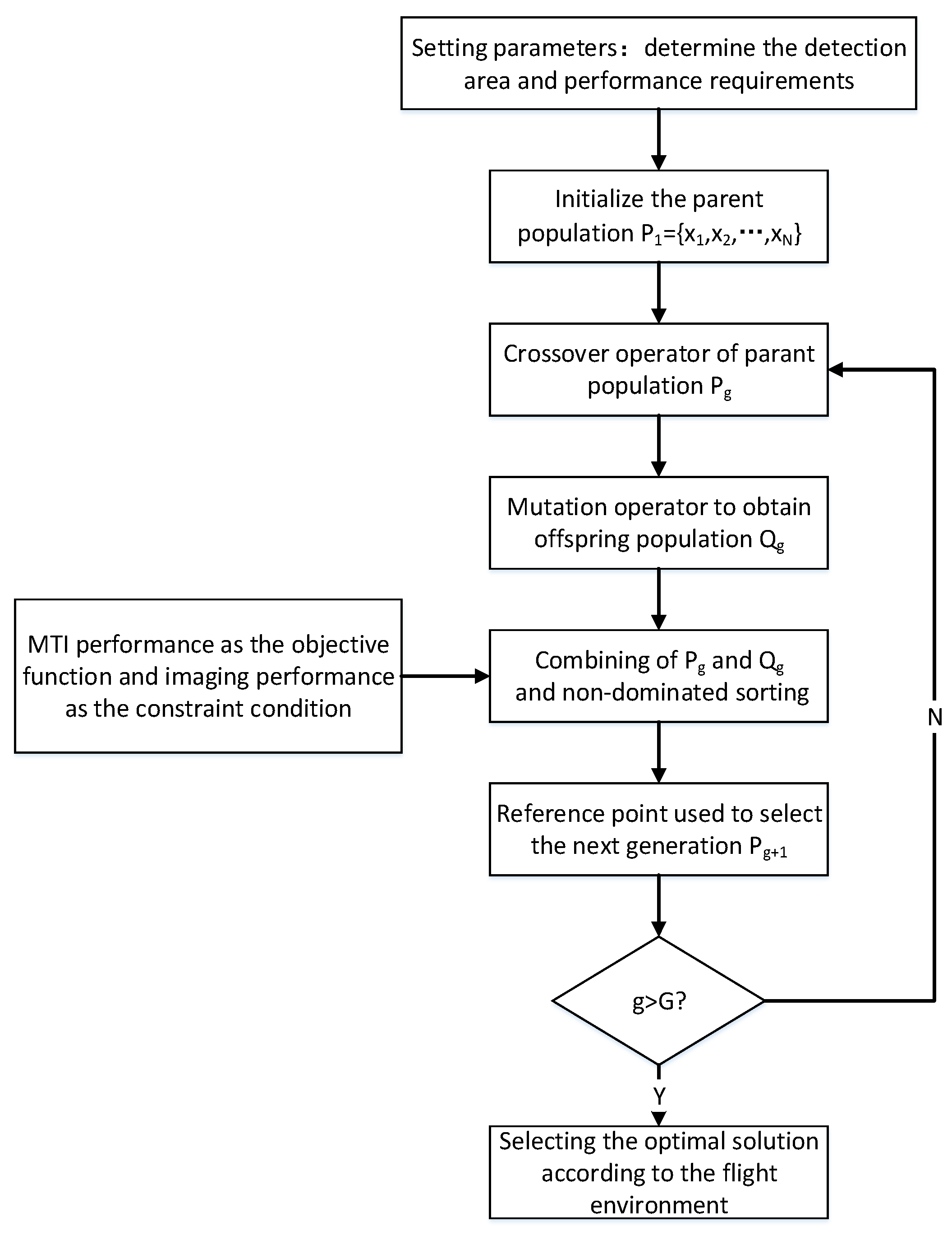
Based on constrained NSGA III algorithm, the specific steps of GEO SA-BSAR MTI system configuration design method are as follows (the flow chart is shown in Figure 2):

Step 1: setting parameters. According to the chosen observation area, the GEO SAR’s trajectory is determined by ephemeris, which guarantee the region can always be illuminated by GEO SAR during the synthetic aperture time. Then, MTI and imaging performance requirements are given. The minimum MUV that can be tolerated is $v_{r\_\max \_\mathrm{Re}}$, the upper limit of range resolution is ${\rho }_{gr\_\mathrm{Re}}$, the upper limit of azimuth resolution is ${\rho }_{az\_\mathrm{Re}}$ and the maximum error of resolution direction angle is $\epsilon$.

Step 2: initialize the parent population. The initial population $P_1=\left\{x_1,x_2,\dots ,x_N\right\}$ composed of $N$ individuals is generated randomly within the range of variable $x={\left({\theta }_R,\varphi ,\psi \right)}^T$.

Step 3: conducting the NSGA III algorithm until the number of iterations reaches the number of genetic $G$.

Step 3.1: for the $g$-th generation, the obtained parent population is $P_g$. In $P_g$, two individuals are randomly selected. Then, the crossover operator is used to simulate the two-point crossover, and the mutation operator is executed under a certain probability to obtain the offspring individuals. Finally, the offspring population containing $N$ individuals is obtained.

Step 3.2: combine the parent population $P_g$ and offspring population $Q_g$ to obtain population $R_g$. The objective function value of every individual in the population $R_g$ is computed by Equation (44). The optimization indicators including the MDV, velocity and location accuracy, as well as the constraint conditions including range resolution, azimuth resolution, resolution direction angle and MUV. The solutions satisfy the constraint conditions as the feasible solution, while the dissatisfied solution as the infeasible solution. Based on the non-dominated sorting, the feasible solution can be divided into several different levels $F_1,F_2,\dots ,F_T$. The infeasible solutions that are ordered according to the error that does not meet the constraint conditions, is arranged after the feasible solutions.

Step 3.3: add the solutions of each levels to the $P_{g+1}$ in order until the number of individuals in $P_{g+1}$ exceeds $N$ for the first time. If the last level added into $P_{g+1}$ is $F_L$, and the number of individuals in $F_L$ causes the number of individuals in $P_{g+1}$ to exceed $N$. Then, based on the method of reference point, each individual in the group $F_L$ is associated with the reference point. The individual nearest to the reference point is selected or randomly selected into $P_{g+1}$. Finally, the next generation of parent population $P_{g+1}$ with $N$ individuals is obtained.

Step 4: select the optimal solution. After the $G$-th iteration, the non-dominant solution set was selected as the optimal solution set from the population $P_G$. Finally, according to the flight environment, the most suitable solution was selected as the bistatic configuration of the real GEO SA-BSAR MTI system.

5. Simulation Verification

In this section, the influence of configuration parameters on the performance of GEO SA-BSAR MTI system is analyzed through simulation. Then, according to the modeling of multi-objective target function with constraint conditions, the optimal bistatic configuration of GEO SA-BSAR MTI system is obtained based on NSGA III algorithm. The system parameters and orbit parameters of the simulated GEO SA-BSAR MTI system are shown in Table 1. In addition, the calculation of ground clutter RCS is modeled as a random rough surface bistatic electromagnetic scattering theory problem [34], and the electromagnetic characteristic parameters used for modeling are also shown in

Table 3. System and electromagnetic characteristic parameters of GEO SA-BSAR MTI system.

System Parameters		Electromagnetic Characteristic Parameter
Peak transmitting power	5000 W	Root mean square height	1.002 cm
Noise temperature	300 K	Correlation length	21.34 cm
Transmitting antenna gain	50 dB	Complex dielectric constant	7
Receiving antenna gain	20.8 dB	Polarization mode	VV
Propagation loss	3.5 dB
Noise figure	4 dB	Rough surface probability distribution	exponential
Duty ratio	0.4

[26].

5.1. Output SCNR Loss Analysis

SCNR loss is one of the important performance indicators and it varies with ${\theta }_R$ and $\varphi$. SCNR loss of the first four configurations of GEO SA-BSAR MTI in

Table 4. Different configuration parameters of GEO SA-BSAR MTI system.

No.	1	2	3	4	5	6	7	8
${\theta }_R$ (deg)	35	60	35	60	35	60	35	60
$\varphi$ (deg)	0	0	150	150	0	0	150	150
$\psi$ (deg)	0	0	0	0	140	140	140	140

will be simulated. The simulation results are in Figure 3, where the solid line is the results by the patch-based approach (calculating SCNR loss by exploiting the echoes of moving target and clutter patches [38]) while the ‘*’ is calculated by using Equation (22). It can be seen that the analytical expression and the actual curve are fitting very well, which can be used to calculate the MDV and MUV.

From the Figure 3, it can be seen that the output SCNR loss curve may have several notches. The target with the velocity at the notch will be suppressed and cannot be detect. Under different GEO SA-BSAR bistatic configurations, the size and position of the notch of output SCNR loss curve will change, resulting in different MDV and MUV caused by the baseline length. It is worth noting that through the de-aliasing algorithm, the pulse repetition frequency (PRF) of the system is essentially increased, and the original 100 Hz PRF is expanded to 300 Hz. At this time, the minimum value of the MUV caused by low PRF under different configuration parameters is 36 m/s, which is already greater than the velocity of most targets, so it is not considered here.

Next, the influences of configuration parameters on the MDV and MUV are analyzed in detail. From the above theoretical analysis, it can be seen that the MDV and MUV of the GEO SA-BSAR MTI system are affected by configuration parameters $\Vert r_{bi}\Vert$, which are determined by the airplane’s incident angle ${\theta }_R$ and the ground projection of the bistatic angle $\varphi$. Figure 4a,b shows the change of the MDV and MUV of GEO SA-BSAR MTI system with ${\theta }_R$ and $\varphi$. From Figure 4a,b, it can be seen that the MDV and the MUV will increase and decrease together with the change of configuration parameters. That means when the configuration make MDV the smallest, the MUV is also small. In addition, there are more than one group of configurations that satisfy the same MUV and MDV. The MDV of most configuration parameters is less than 3 m/s, where the MUV of some configurations is less than 20 m/s, which is difficult to meet the actual demand. Since the MDV and the MUV are unable to be optimal at the same time, we make the MUV greater than a certain value and minimize the MDV when obtaining the optimal bistatic configuration.

The MDV and MUV for different airplane’s velocities are also shown in Figure 4, where (a) and (b) are results for the airplane’s velocity with 150 m/s, (c) and (d) for 200 m/s, (e) and (f) for 250 m/s. It can be seen that with increasing of airplane’s velocity, both the MDV and MUV become greater. It can also be proved by the expressions in Equations (24) and (26). Thus, when we need to detect target with large velocity, such as the vehicles on the highway, the higher airplane’s velocity can be selected.

5.2. CRLB Analysis

Another important MTI performance indicator is CRLB. The analytical expression of CRLB is hard to be given. We intend to adopt numerical simulation to show the relationship between the CRLB and bistatic configuration parameters. Firstly, we choose 8 bistatic configurations in Table 4 to simulate their CRLBs. Their CRLBs are shown in Figure 5, where (a) and (b) are the CRLBs for radial velocity and (c) and (d) are the CRLBs for azimuth position. It is obvious that the CRLB for radial velocity varies with ${\theta }_R$ and $\varphi$, but $\psi$ has little effect, while the CRLB for azimuth position is impacted by ${\theta }_R$, $\varphi$ and $\psi$ at the same time. Considering that CRLBs vary with radial velocity, their maximum values are used to compare different configurations’ performance. For Figure 5a,b, it can be seen that ${\theta }_R$ and $\varphi$ influence the priority of these configuration according to the CRLBs for radial velocity, while $\psi$ hardly changes the priority but has impacts on the values. For Figure 5c,d, it can be seen that ${\theta }_R$, $\varphi$ and $\psi$ determine the priority of these configuration according to the CRLBs for azimuth position together.

Further, the estimation accuracies according to the CRLBs are analysis. Considering that CRLB varies with radial velocity, their maximum values are analyzed. Figure 6 shows the variation of the velocity accuracy and location accuracy of the target with the ground projection of bistatic angle and airplane’s incidence angle when the ground projection of velocity angle is 0. Figure 7 shows the variation of the velocity accuracy and location accuracy with the ground projection of velocity angle and airplane’s incidence angle when the bistatic angle is 0. In Figure 6 and Figure 7, in order to better display the variation of velocity accuracy and location accuracy in most configurations, the variation range of color bar is restricted. In fact, when configuration parameters are not selected correctly, the velocity accuracy can reach 671 m/s, while the location accuracy can reach 5120 km. It can be seen from the variation trend of Figure 6 and Figure 7 that the location accuracy may be large even if the velocity accuracy is small, and the location accuracy and velocity measurement accuracy are not increasing or decreasing in the same direction. The accuracy is non-convex with the change of configuration parameters, so the genetic algorithm can be used to solve this non-convex optimization problem. In addition, the performance results for different airplane’s velocities are also shown in Figure 6 and Figure 7, where (a) and (b) are the results for the airplane’s velocity of 150 m/s, (c) and (d) for 200 m/s, (e) and (f) for 250 m/s. With the increasing of the airplane’s velocity, there are more bistatic configurations that have large radial velocity estimation errors, while the bistatic configurations with large location errors become less. For different airplane’s velocities, the bistatic configurations with low radial velocity and location accuracies still exist to achieve MTI.

5.3. Bistatic Configuration Design Results

From simulation of MTI performance with the change of configuration parameters, because the minimum MDV and maximum MUV cannot be met at the same time and velocity and location accuracy is non-convex, the problems of the configuration design can’t directly to minimize all performance indicators. We minimize the MDV, velocity accuracy and location accuracy under the condition of MDV more than a specified value. In addition, the imaging performance will also be consideration for configuration design as shown in Equation (44).

If it is required that the MUV is not more than 30 m/s, the range resolution no more than 4 m, the azimuth resolution no more than 3 m and the tolerable error of resolution angle is 0.1 rad, according to the parameters of NSGA III algorithm as shown in

Table 5. Simulation parameters of non-dominant sorting genetic algorithm III.

Parameters	Values	Parameters	Values
Population size	100	Number of iterations	500
Mutation probability	0.33	Crossover probability	0.9
Mutation factor	20	Crossover factor	20

, the result of configuration design and the corresponding performance indicators at the equator is shown in

Table 6. Results of configuration design of GEO SA-BSAR MTI system at the equator.

Configuration Number		1	2	3	4
Configuration Parameters	${\theta }_R$ (deg)	19.48	22.24	24.00	27.01
	$\varphi$ (deg)	80.44	75.93	74.97	72.97
	$\psi$ (deg)	204.50	201.64	205.55	205.83
MTI Performance	$v_{r\_MDV}$ (m/s)	3.91	3.86	3.74	3.52
	$v_{r\_MUV}$ (m/s)	35.42	32.95	31.87	30.05
	${\sigma }_{v_r}$ (m/s)	0.055	0.15	0.15	0.16
	${\sigma }_x$ (m)	2.22	6.42	7.36	8.52
Imaging Performance	${\rho }_{gr}$ (m)	3.92	3.65	3.53	3.32
	${\rho }_{az}$ (m)	1.22	1.26	1.28	1.33

. By once solving processing, several bistatic configurations that meet the requirement of MUV, range resolution, azimuth resolution and resolution direction angle are obtained. Configuration 1 can achieve the MDV of about 3.91 m/s, the location accuracy is about 2.22 m and the velocity accuracy is about 0.055 m/s.

The results of configuration design and the corresponding performance indicators at the perigee are shown in

Table 7. Results of configuration design of GEO SA-BSAR MTI system at the perigee.

Configuration Number		1	2	3
Configuration Parameters	${\theta }_R$ (deg)	19.48	21.61	22.21
	$\varphi$ (deg)	80.45	76.33	75.98
	$\psi$ (deg)	205.78	200.26	210.55
MTI Performance	$v_{r\_MDV}$ (m/s)	3.92	3.91	3.86
	$v_{r\_MUV}$ (m/s)	35.42	33.36	32.97
	${\sigma }_{v_r}$ (m/s)	0.056	0.14	0.15
	${\sigma }_x$ (m)	2.22	6.08	6.30
Imaging Performance	${\rho }_{gr}$ (m)	3.92	3.69	3.65
	${\rho }_{az}$ (m)	1.21	1.26	1.23

. Configuration 1 can achieve the MDV of about 3.92 m/s, the location accuracy is about 2.22 m and the velocity accuracy is about 0.056 m/s. In addition, the results at the middle position between the equator and the perigee are shown in

Table 8. Results of configuration design of GEO SA-BSAR MTI system at the middle position.

Configuration Number		1	2	3
Configuration Parameters	${\theta }_R$ (deg)	19.48	22.07	28.44
	$\varphi$ (deg)	279.49	283.93	284.02
	$\psi$ (deg)	153.64	148.77	146.97
MTI Performance	$v_{r\_MDV}$ (m/s)	3.92	3.88	3.52
	$v_{r\_MUV}$ (m/s)	35.44	33.06	30.02
	${\sigma }_{v_r}$ (m/s)	0.056	0.15	0.13
	${\sigma }_x$ (m)	2.17	6.20	6.78
Imaging Performance	${\rho }_{gr}$ (m)	3.92	3.66	3.65
	${\rho }_{az}$ (m)	1.21	1.23	1.23

. Configuration 1 can achieve the MDV of about 3.92 m/s, the location accuracy is about 2.17 m and the velocity accuracy is about 0.056 m/s. From the results of the different GEO SAR orbital positon, it can be seen that the optimal performances for different orbital location are similar. It results from the different orbital position lead to different GEO SAR velocity, which has little impacts on the MTI performance. Thus, the location of GEO SAR will not change the performance of GEO SA-BSAR MTI system.

6. Conclusions

In this paper, a configuration design method for GEO SA-BSAR MTI system is proposed. Based on the optimal SNR criterion, the analytical expressions of MDV and MUV in terms of configuration parameters are derived, which is determined by the airplane’s incident angle and the ground projection of bistatic angle. The CRLBs for radial velocity and azimuth position depends on the airplane’s incident angle, the ground projection of bistatic angle and velocity angle. According to the characteristic of MTI performance, the multi-objective optimization problem with constraint conditions is modelled to obtain the optimal bistatic configuration of GEO SA-BSAR system. Then, the NSGA III algorithm is exploited to obtain multiple optimal bistatic configuration for GEO SA-BSAR MTI system with the given lower limit of MUV, the upper limit of range resolution, the upper limit of the azimuth resolution and maximum error of resolution angle. The flight environment help to choose the most appropriate bistatic configuration. For a ‘small 8’ GEO orbit, after the configuration design, the MDV is about 3.91 m/s, the location accuracy is about 6.08 m and the velocity accuracy is about 0.14 m/s. In the future, we will further study the data processing of GEO SA-BSAR MTI system.

References

1. Gabriel, A.K.; Goldstein, R.M. Bistatic images from SIR-B. In Proceedings of the International Geoscience and Remote Sensing Symposium, Amherst, MA, USA, 7–9 October 1985; p. 112. [Google Scholar]
2. Espeter, T.; Walterscheid, I.; Klare, J.; Ender, J.H.G. Synchronization techniques for the bistatic spaceborne/airborne SAR experiment with TerraSAR-X and PAMIR. In Proceedings of the IEEE International Geoscience & Remote Sensing Symposium, Barcelona, Spain, 23–28 July 2007; pp. 2160–2163. [Google Scholar]
3. Espeter, T.; Walterscheid, I.; Klare, J.; Gierull, C.; Brenner, A.; Ender, J.; Loffeld, O. Progress of Hybrid Bistatic SAR: Synchronization Experiments and First Imaging Results. In Proceedings of the 7th European Conference on Synthetic Aperture Radar, Friedrichshafen, Germany, 2–5 June 2008. [Google Scholar]
4. Walterscheid, I.; Espeter, T.; Ender, J.H.G. Performance analysis of a hybrid bistatic SAR system operating in the double sliding spotlight mode. In Proceedings of the 2007 IEEE International Geoscience and Remote Sensing Symposium, Barcelona, Spain, 23–28 July 2007. [Google Scholar]
5. Rodriguezcassola, M.; Baumgartner, S.V.; Krieger, G.; Nottensteiner, A.; Horn, R.; Steinbrecher, U.; Metzig, R.; Limbach, M.; Prats, P.; Fischer, J.V.; et al. Bistatic spaceborne-airborne experiment TerraSAR-X/F-SAR: Data processing and results. In Proceedings of the 2008 IEEE International Geoscience and Remote Sensing Symposium, Boston, MA, USA, 7–11 July 2008. [Google Scholar]
6. Baumgartner, S.V.; Rodriguez-Cassola, M.; Nottensteiner, A.; Horn, R.; Scheiber, R.; Schwerdt, M.; Steinbrecher, U.; Metzig, R.; Limbach, M.; Mittermayer, J.; et al. Bistatic Experiment Using TerraSAR-X and DLR’s new F-SAR System. In Proceedings of the 7th European Conference on Synthetic Aperture Radar, Friedrichshafen, Germany, 2–5 June 2008. [Google Scholar]
7. Walterscheid, I.; Espeter, T.; Klare, J.; Nies, H.; Brenner, A.R.; Ender, J.H.G.; Wang, R.; Loffeld, O.D. Bistatic SAR Experiments with PAMIR and TerraSAR-X—Setup, Processing, and Image Results. IEEE Trans. Geosci. Remote Sens. 2010, 48, 3268–3279. [Google Scholar] [CrossRef]
8. Hong, F.; Wang, R.; Zhang, A.; Lu, P.; Balz, T. Integrated time and phase synchronization strategy for a multichannel spaceborne-stationary bistatic SAR system. Remote Sens. 2016, 8, 628. [Google Scholar] [CrossRef] [Green Version]
9. Long, T.; Hu, C.; Ding, Z.; Dong, X.; Tian, W.; Zeng, T. Geosynchronous SAR: System and Signal. Processing; Springer: Singapore, 2018. [Google Scholar]
10. Long, T.; Dong, X.; Hu, C.; Zeng, T. A New Method of Zero-Doppler Centroid Control in GEO SAR. IEEE Geosci. Remote Sens. Lett. 2011, 8, 512–516. [Google Scholar] [CrossRef]
11. Hu, C.; Zhang, B.; Dong, X.; Li, Y. Geosynchronous SAR Tomography: Theory and First Experimental Verification Using Beidou IGSO Satellite. IEEE Trans. Geosci. Remote Sens. 2019, 57, 6591–6607. [Google Scholar] [CrossRef]
12. Ruiz-Rodon, J.; Broquetas, A.; Makhoul, E.; Guarnieri, A.M.; Rocca, F. Nearly Zero Inclination Geosynchronous SAR Mission Analysis with Long Integration Time for Earth Observation. IEEE Trans. Geosci. Remote Sens. 2014, 52, 6379–6391. [Google Scholar] [CrossRef]
13. Cui, W.; Tian, J.; Xia, X.-G.; Wu, S. An approach for parameter estimation of maneuvering targets with nonlinear motions. IEEE Trans. Aerosp. Electron. Syst. 2020, 56, 67–83. [Google Scholar] [CrossRef]
14. Hobbs, S.; Sanchez, J.P. Laplace plane and low inclination geosynchronous radar mission design. Sci. China Inf. Sci. 2017, 60, 060305. [Google Scholar] [CrossRef]
15. Hu, C.; Long, T.; Zeng, T.; Liu, F.; Liu, Z. The Accurate Focusing and Resolution Analysis Method in Geosynchronous SAR. IEEE Trans. Geosci. Remote Sens. 2011, 49, 3548–3563. [Google Scholar] [CrossRef]
16. Hu, C.; Chen, Z.; Dong, X.; Cui, C. Multistatic Geosynchronous SAR Resolution Analysis and Grating Lobe Suppression Based on Array Spatial Ambiguity Function. IEEE Trans. Geosci. Remote Sens. 2020. early access. [Google Scholar] [CrossRef]
17. Dong, X.; Hu, J.; Hu, C.; Long, T.; Li, Y.; Tian, Y. Modeling and Quantitative Analysis of Tropospheric Impact on Inclined Geosynchronous SAR Imaging. Remote Sens. 2019, 11, 803. [Google Scholar] [CrossRef] [Green Version]
18. Hu, C.; Liu, Z.; Long, T. An improved focusing method for geosynchronous SAR. Adv. Space Res. 2013, 51, 1773–1783. [Google Scholar] [CrossRef]
19. Hu, C.; Li, Y.; Dong, X.; Wang, R.; Cui, C. Optimal 3D deformation measuring in inclined geosynchronous orbit SAR differential interferometry. Sci. China Inf. Sci. 2017, 60, 060303. [Google Scholar] [CrossRef]
20. Zhang, Y.; Xiong, W.; Dong, X.; Hu, C. A Novel Azimuth Spectrum Reconstruction and Imaging Method for Moving Targets in Geosynchronous Spaceborne-Airborne Bistatic Multichannel SAR. IEEE TGRS 2020. early access. [Google Scholar] [CrossRef]
21. Melzi, M.; Hu, C.; Dong, X.; Li, Y.; Cui, C. Velocity Estimation of Multiple Moving Targets in Single-Channel Geosynchronous SAR. IEEE TGRS 2020. early access. [Google Scholar] [CrossRef]
22. Zhang, Y.; Xiong, W.; Dong, X.; Hu, C.; Sun, Y. GRFT-Based Moving Ship Target Detection and Imaging in Geosynchronous SAR. Remote Sens. 2018, 10, 2002. [Google Scholar] [CrossRef] [Green Version]
23. Guttrich, G.; Sievers, W. Wide area surveillance concepts based on geosynchronous illumination and bistatic UAV or satellite reception. In Proceedings of the IEEE Aerospace Conference, Snowmass at Aspen, CO, USA, 13 February 1997. [Google Scholar]
24. Wu, J.; Sun, Z.; Huang, Y.; Yang, J.; Lv, Y.; Wang, Z. Geosynchronous spaceborne-airborne bistatic SAR: Potentials and prospects. In Proceedings of the Radar Conference, Arlington, VA, USA, 10–15 May 2015. [Google Scholar]
25. Sun, Z.; Wu, J.; Huang, Y.; Yang, J.; Yang, H.; Yang, X. Performance analysis and mission design for inclined geosynchronous spaceborne-airborne bistatic SAR. In Proceedings of the Radar Conference, Arlington, VA, USA, 10–15 May 2015. [Google Scholar]
26. Sun, Z.; Wu, J.; Pei, J.; Li, Z.; Huang, Y.; Yang, J. Inclined Geosynchronous Spaceborne–Airborne Bistatic SAR: Performance Analysis and Mission Design. IEEE Trans. Geosci. Remote Sens. 2016, 54, 343–357. [Google Scholar] [CrossRef]
27. Wu, J.; Sun, Z.; Zhang, Q.; An, H.; Yang, J.; Li, C.; Li, D. Geosynchronous spaceborne-airborne bistatic SAR for earth observation: Advantages and main aspects. In Proceedings of the 2016 IEEE 13th International Conference on Signal Processing (ICSP), Chengdu, China, 6–10 November 2016. [Google Scholar]
28. Wu, J.; Sun, Z.; Li, Z.; Huang, Y.; Yang, J.; Liu, Z. Focusing Translational Variant Bistatic Forward-Looking SAR Using Keystone Transform and Extended Nonlinear Chirp Scaling. Remote Sens. 2016, 8, 840. [Google Scholar] [CrossRef] [Green Version]
29. An, H.; Wu, J.; Sun, Z.; Yang, J. A Two-Step Nonlinear Chirp Scaling Method for Multichannel GEO Spaceborne-Airborne Bistatic SAR Spectrum Reconstructing and Focusing. IEEE Trans. Geosci. Remote Sens. 2019, 57, 3713–3728. [Google Scholar] [CrossRef]
30. Wu, J.; Sun, Z.; An, H.; Qu, J.; Yang, J. Azimuth Signal Multichannel Reconstruction and Channel Configuration Design for Geosynchronous Spaceborne-Airborne Bistatic SAR. IEEE Trans. Geosci. Remote Sens. 2018, 57, 1861–1872. [Google Scholar] [CrossRef]
31. Li, G.; Xu, J.; Peng, Y.-N.; Xia, X.-G. Bistatic Linear Antenna Array SAR for Moving Target Detection, Location, and Imaging with Two Passive Airborne Radars. IEEE Trans. Geosci. Remote Sens. 2007, 45, 554–565. [Google Scholar] [CrossRef]
32. Zeng, T.; Cherniakov, M.; Long, T. Generalized approach to resolution analysis in BSAR. IEEE Trans. Aerosp. Electron. Syst. 2005, 41, 461–474. [Google Scholar] [CrossRef]
33. Li, T.; Chen, K.-S.; Jin, M. Analysis and Simulation on Imaging Performance of Backward and Forward Bistatic Synthetic Aperture Radar. Remote Sens. 2018, 10, 1676. [Google Scholar] [CrossRef] [Green Version]
34. Fung, A.; Liu, W.; Chen, K.; Tsay, M. An improved IEM model for bistatic scattering from rough surfaces. J. Electromagn. Waves Appl. 2002, 16, 689–702. [Google Scholar] [CrossRef]
35. Mhetre, P.S. Genetic algorithm for linear and nonlinear equation. Int. J. Adv. Eng. Technol. 2012, 3, 114–118. [Google Scholar]
36. Deb, K.; Pratap, A.; Agarwal, S.; Meyarivan, T. A fast and elitist multiobjective genetic algorithm: NSGA-II. IEEE Trans. Evol. Comput. 2002, 6, 182–197. [Google Scholar] [CrossRef] [Green Version]
37. Wong, F.; Cumming, I.; Neo, Y.L. Focusing Bistatic SAR Data Using the Nonlinear Chirp Scaling Algorithm. IEEE Trans. Geosci. Remote Sens. 2008, 46, 2493–2505. [Google Scholar] [CrossRef] [Green Version]
38. Fertig, L.B. Analytical expressions for space-time adaptive processing (STAP) performance. IEEE Trans. Aerosp. Electron. Syst. 2015, 51, 42–53. [Google Scholar] [CrossRef]
39. Cerutti-Maori, D.; Sikaneta, I.; Gierull, C.H. Optimum SAR/GMTI Processing and Its Application to the Radar Satellite RADARSAT-2 for Traffic Monitoring. IEEE Trans. Geosci. Remote Sens. 2012, 50, 3868–3881. [Google Scholar] [CrossRef]
40. Gierull, C.H.; Cerutti-Maori, D.; Ender, J. Ground Moving Target Indication with Tandem Satellite Constellations. IEEE Geosci. Remote Sens. Lett. 2008, 5, 710–714. [Google Scholar] [CrossRef]
41. Deb, K.; Jain, H. An Evolutionary Many-Objective Optimization Algorithm Using Reference Point-Based Nondominated Sorting Approach, Part I: Solving Problems with Box Constraints. IEEE Trans. Evol. Comput. 2014, 18, 577–601. [Google Scholar] [CrossRef]
Figure 1. The local coordinate system of geosynchronous (GEO) spaceborne-airborne (SA)-bistatic synthetic aperture radar (BSAR) moving target indication (MTI) system.
Remotesensing 12 01810 g001
Figure 2. Configuration design flow chart of GEO SA-BSAR MTI system.
Remotesensing 12 01810 g002
Figure 3. Signal to clutter and noise ratio (SCNR) loss for different bistatic configuration: (a) configuration 1 and configuration 2; (b) configuration 3 and configuration 4.
Remotesensing 12 01810 g003
Figure 4. The variation of minimum detectable velocity (MDV) and maximum unambiguous velocity (MUV) with configuration parameters for different airplane’s velocities: (a) MDV for the airplane’s velocity of 150 m/s; (b) MUV for the airplane’s velocity of 150 m/s; (c) MDV for the airplane’s velocity of 200 m/s; (d) MUV for the airplane’s velocity of 200 m/s; (e) MDV for the airplane’s velocity of 250 m/s; (f) MUV for the airplane’s velocity of 250 m/s.
Remotesensing 12 01810 g004aRemotesensing 12 01810 g004b
Figure 5. Cramer–Rao lower bounds (CRLBs) for radial velocity and azimuth position of different bistatic configurations: (a) CRLBs for radial velocity of configurations 1~4; (b) CRLBs for radial velocity of configurations 5~6; (c) CRLBs for azimuth position of configuration 1~4; (d) CRLBs for azimuth position of configurations 5~6.
Remotesensing 12 01810 g005aRemotesensing 12 01810 g005b
Figure 6. When the velocity angle is 0, the variation of velocity and location accuracy with the receiver’s incidence angle and the ground projection of the bistatic angle for different airplane’s velocities: (a) the variation of velocity accuracy for the airplane’s velocity of 150 m/s; (b) the variation of location accuracy for the airplane’s velocity of 150 m/s; (c) the variation of velocity accuracy for the airplane’s velocity of 200 m/s; (d) the variation of location accuracy for the airplane’s velocity of 200 m/s; (e) the variation of velocity accuracy for the airplane’s velocity of 250 m/s; (f) the variation of location accuracy for the airplane’s velocity of 250 m/s.
Remotesensing 12 01810 g006aRemotesensing 12 01810 g006b
Figure 7. When the ground projection of bistatic angle is 0, the variation of velocity and location accuracy with the receiver’s incidence angle and ground projection of velocity angle for different airplane’s velocities: (a) the variation of velocity accuracy for the airplane’s velocity of 150 m/s; (b) the variation of location accuracy for the airplane’s velocity of 150 m/s; (c) the variation of velocity accuracy for the airplane’s velocity of 200 m/s; (d) the variation of location accuracy for the airplane’s velocity of 200 m/s; (e) the variation of velocity accuracy for the airplane’s velocity of 250 m/s; (f) the variation of location accuracy for the airplane’s velocity of 250 m/s.
Remotesensing 12 01810 g007aRemotesensing 12 01810 g007b