Article

Azimuth Multichannel Reconstruction for Moving Targets in Geosynchronous Spaceborne–Airborne Bistatic SAR

1
College of Information Engineering, Inner Mongolia University of Technology, Hohhot 010050, Inner Mongolia, China
2
Inner Mongolia Key Laboratory of Radar Technology and Application, Hohhot 010050, Inner Mongolia, China
3
Chinese Academy of Space Technology, Qian Xuesen Laboratory of Space Technology, Beijing 100094, China
*
Author to whom correspondence should be addressed.
Remote Sens. 2020, 12(11), 1703; https://doi.org/10.3390/rs12111703
Submission received: 23 April 2020 / Revised: 21 May 2020 / Accepted: 25 May 2020 / Published: 26 May 2020

Abstract

:
In a multichannel geosynchronous spaceborne–airborne bistatic synthetic aperture radar (GEO-SA-BiSAR) system, the airborne receiver can obtain high-resolution microwave images with good signal-to-noise ratios (SNRs) by passively receiving echoes from the desired area. Since the Doppler modulation and range history of a moving target are obviously different from a stationary target, a signal geometry model for moving targets in multichannel GEO-SA-BiSAR is established in this paper. According to simulation results, the along track velocity introduces target defocusing in azimuth, and the slant range velocity mainly causes multiple false targets. To resolve these problems, a modified multichannel reconstruction method in azimuth channel GEO-SA-BiSAR is proposed according to the azimuth multichannel impulse response of the imaged moving target. Before azimuth multichannel raw data combination, both spatial-variant range cell migration correction (RCMC) and azimuth nonlinear chirp scaling (ANLCS) should be performed to reduce the influence of the range offset and lower the Doppler bandwidth of the whole raw data, respectively. Afterward, a novel azimuth multichannel reconstruction algorithm is carried out via the modified reconstruction matrix based on the estimated target velocity. The target slant range velocity estimation is implemented by introducing the signal intensity ratio (SIR). Compared with the conventional method for the stationary target to handle the raw data of the moving target, the false targets could be obviously suppressed by using the proposed approach. Imaging results on both simulated point and distributed scene targets validate the proposed multichannel reconstruction approach.

Graphical Abstract

1. Introduction

Synthetic aperture radar (SAR) can get microwave images of the desired scene under all weather conditions, day and night [1]. For spaceborne SAR, most SAR systems are in a low earth orbit (LEO) at heights ranging from 300 km to 1200 km. With the development of the spaceborne SAR system, the disadvantages of LEO SAR, such as small instantaneous beam coverage and long revisit time, are becoming more and more obvious. To resolve these problems, the concept of geostationary SAR (GEO SAR) was proposed [2,3,4,5], which has an orbit height of nearly 36,500 km. Consequently, compared with LEO SAR, a larger wide-swath could be illuminated with a shorter revisit time by GEO SAR [6,7]. Therefore, GEO SAR has many advantages in military reconnaissance, ocean applications, and earth dynamics [8].
Although GEO SAR could overcome major shortcomings of LEO SAR, it is very difficult to get microwave images with high azimuth resolution and signal-to-noise ratio (SNR) [9]. Fortunately, compared with monostatic GEO SAR with the same transmit peak power, the bistatic SAR imaging scheme consisting of a GEO transmitter and an airborne receiver, named as geosynchronous spaceborne–airborne bistatic synthetic aperture radar (GEO-SA-BiSAR), could obtain SAR images with finer azimuth resolution and higher SNR [10,11]. Furthermore, compared with traditional monostatic SAR systems, the GEO-SA-BiSAR system has enormous advantages, such as well concealment, strong anti-attack ability, real-time SAR imaging capacity, and well flexibility [12,13]. Therefore, the unique characteristics of GEO-SA-BiSAR would make it be widely adopted in future. Compared with conventional LEO SAR, azimuth precisely data focusing in GEO-SA-BiSAR is more difficult. This is because the slant range history is more complex than other SAR systems, and the low operating pulse repetition frequency (PRF) in GEO SAR results in Doppler spectrum aliasing [14]. In GEO-SA-BiSAR systems, phase and time synchronization are very important issues, especially for the imaged scene with the low SNR level. In recent years, multiple phase/time synchronization processing approaches have been proposed [15,16,17]. In the GEO-SA-BiSAR system, the direct-path signal is received as the reference signal by an additional receive channel for phase and time synchronization. For the ocean scene with the low SNR, phase and time synchronization are usually implemented according to strong scatters such as small islands and stationary ships.
The operating PRF of the GEO-SA-BiSAR system is determined by the GEO transmitter, and a low PRF is chosen to obtain wide swath coverage and to lessen the burden of raw data storage onboard and down link transmission. The wide Doppler bandwidth for a fine azimuth resolution depends on the airborne receiver, because the Doppler modulation rate corresponding to the airborne receiver is obviously larger than the GEO transmitter. Therefore, the GEO-SA-BiSAR system brings a contradiction between the low PRF of the transmitter and the wide Doppler bandwidth determined by the receiver. Similar to the high resolution wide swath (HRWS) SAR system [18], the azimuth multichannel imaging scheme could resolve this contradiction by introducing additional azimuth spatial samples. The azimuth multichannel receiving technology is composed of multiple receiving sub-apertures on the receiving airborne platform, which can improve the target Doppler bandwidth for a better azimuth resolution but with a low PRF sampling rate. To combine azimuth multichannel SAR together before the single channel GEO-SA-BiSAR processor, azimuth multichannel reconstruction usually should be taken because of non-uniform sampling. In recent years, multiple reconstruction and imaging approaches for the stationary target have been proposed [19,20,21], but few studies have focused on the moving target in GEO-SA-BiSAR.
Compared with the stationary target in multichannel GEO-SA-BiSAR [22,23], the moving target has a different range history and Doppler modulation [24,25]. If azimuth multichannel reconstruction and imaging approaches for stationary scenes were adopted to handle the echoes of moving targets, imaging quality would be seriously reduced. To resolve this issue, the geometry model of the moving target in GEO-SA-BiSAR is analyzed in this paper, and the effects of the target velocity including the along track and slant range components on the focusing quality are analyzed. According to the azimuth multichannel impulse function, a novel azimuth multichannel reconstruction method for moving targets in GEO-SA-BiSAR is proposed. Before combining azimuth multichannel raw data, spatial-variant range cell migration correction (RCMC) is performed to reduce the influence of the range offset, and the Doppler bandwidth of the whole raw data is decreased via azimuth nonlinear chirp scaling (ANLCS). The key fact of the novel reconstruction approach is the modified reconstruction matrix based on the estimated moving target velocity. The along track velocity component is easily obtained by azimuth data autofocusing similarly to the single-channel SAR system. For the estimation of the slant range velocity component, a signal intensity ratio (SIR) is introduced to describe the ratio between the in-band and out-of-band signal after azimuth multichannel reconstruction with the estimated target velocity [26,27]. After azimuth multichannel reconstruction with the accurate target velocity, the moving target is well focused via the traditional image processing technique for moving targets, and its corresponding false targets due to the target velocity are obviously suppressed.
This paper is organized as follows. The signal model of the moving target in azimuth multichannel GEO-SA-BiSAR is established in Section 2. The effects of the moving target velocity on the target focusing quality are analyzed in Section 3. The proposed reconstruction approach is presented in detail in Section 4. Simulation results for both point and distributed targets are analyzed in Section 5 to validate the proposed reconstruction approach. Conclusions are reported in Section 6.

2. Geometry and Azimuth Signal Model for Moving Targets in GEO-SA-BiSAR

Because of the low operating PRF in GEO SAR, the azimuth raw data would be under-sampled and its spectrum would be aliased, if an azimuth signal with a large azimuth bandwidth were received by the airborne platform. There are two ways to resolve this contradiction. The first way is to improve the operating PRF value of the GEO SAR system, although this raises system complexity. The other way is to use azimuth multichannel reception technology on the airborne receiving platform to increase azimuth spatial samplings. The azimuth multichannel reception technique can improve the effective azimuth sampling rate without increasing PRF, and it has been implemented by multiple airborne/spaceborne SAR systems.

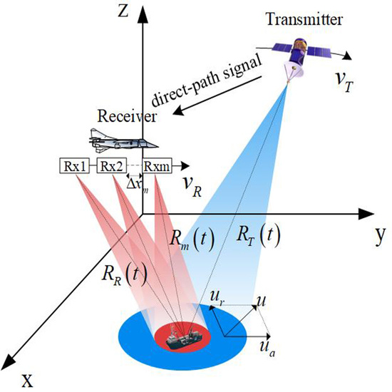
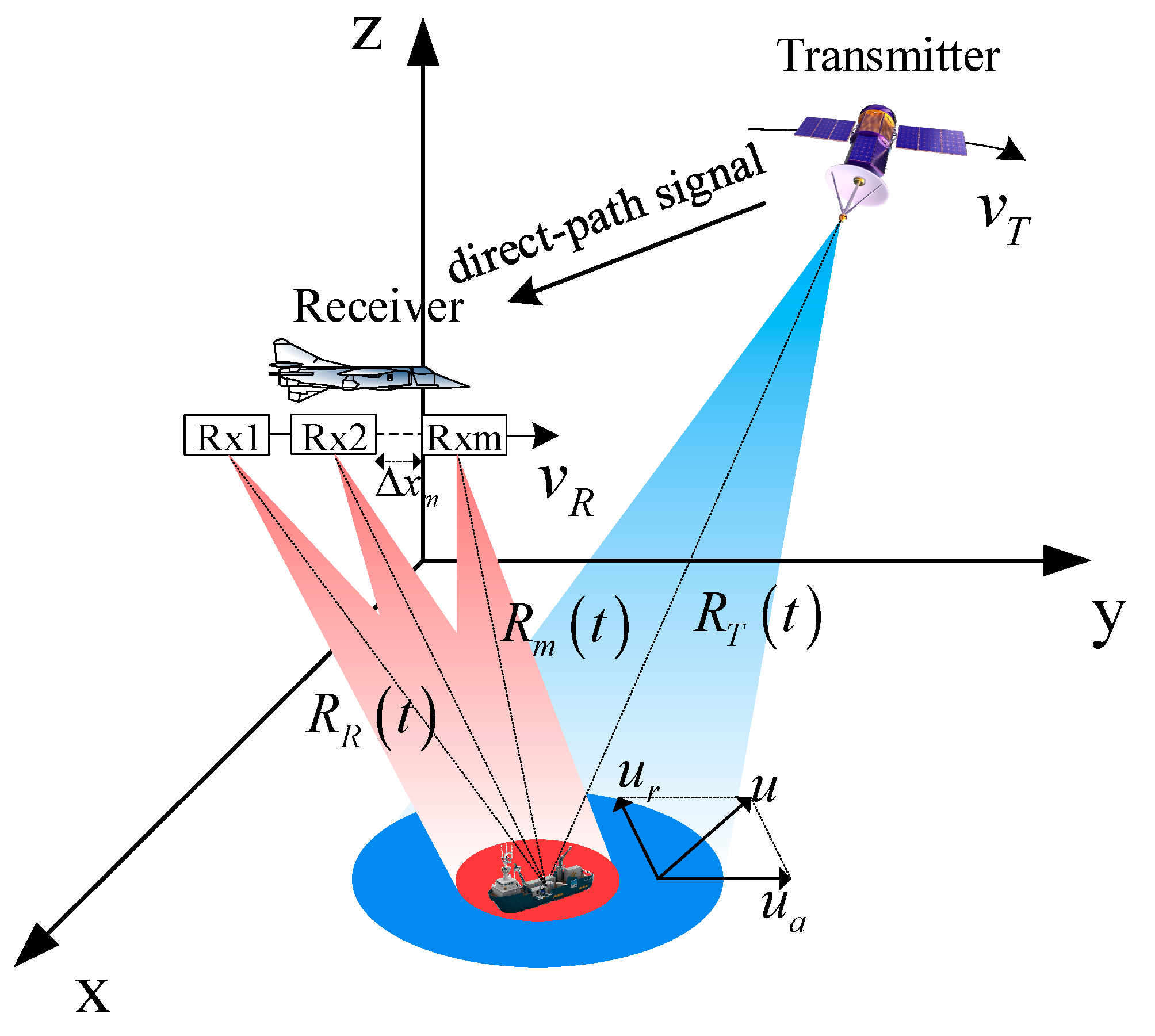
2.1. Geometry and Slant Range

The moving target imaging geometry in GEO-SA-BiSAR is illustrated in Figure 1. GEO SAR transmits radar signals, and the airborne receiver receives echoes reflected by the moving target. The GEO SAR moves with the velocity v T , and the velocity of the airborne is v R in the y-direction. The direct-path signal from the GEO transmitter is received by the airborne platform for time/phase synchronization. The M receiving sub-apertures are aligned in azimuth, and the physical interval between the m-th receiving sub-aperture and the reference is Δ x m . The target velocity u decomposes into the along track component u a and the slant range component u r for the convenience of subsequent analysis. The range R R ( t ) from the airborne receiving phase center to the illuminated moving target could be written as
R R ( t ) = ( R 0 u r t ) 2 + ( v r v t ) 2
with
v r v = v R u a
where R 0 denotes the shortest slant range from the receiver to the imaged moving target, and t is the azimuth time. The slant range history of (1) can be expanded into a Taylor series as follows:
R R ( t ) R 0 + u r 2 + v r v 2 2 R 0 ( t u r R 0 u r 2 + v r v 2 ) 2 u a 2 + v r v 2 2 R 0 ( u r R 0 u r 2 + v r v 2 ) 2
Similar to (1), the slant range history R m ( t ) for the m-th receiving channel in azimuth can be expressed as
R m ( t ) = ( R 0 u r t ) 2 + ( v r v t Δ x m ) 2
The slant range history of (4) expanded into a Taylor series can be expressed as
R m ( t ) R 0 + u r 2 + v r v 2 2 R 0 ( t u r R 0 u r 2 + v r v 2 v r v Δ x m u r 2 + v r v 2 ) 2 u r 2 + v r v 2 2 R 0 ( R 0 u r + v r v Δ x m u r 2 + v r v 2 ) 2 + 1 2 R 0 Δ x m 2
Combining (3) with (5), the following expression can be obtained:
R m ( t ) = R R ( t v r v Δ x m u r 2 + v r v 2 ) + Δ R R
with
Δ R R = 1 2 R 0 ( Δ x m 2 v r v 2 Δ x m 2 + 2 R 0 u r v r v Δ x m u r 2 + v r v 2 )
For a GEO SAR with a high orbit, a fourth-order approximation of R T ( t ) is usually modeled and established to accurately estimate the actual slant range between the GEO SAR system and the target with a long synthetic aperture time [28], and it is written as
R T ( t ) R 1 T + k 1 T t + k 2 T t 2 + k 3 T t 3 + k 4 T t 4
where R 1 T denotes the shortest distance between the moving target and the GEO transmitter, and k n T ( n = 1 , 2 , 3 , 4 ) represents the polynomial coefficients of the n-th order. However, the synthetic aperture time of the GEO-SA-BiSAR system is much smaller than monostatic GEO-SAR, and the phase errors caused by the last two terms are less than 1 × 10 4 π [24], which could be neglected. Consequently, R T ( t ) in (8) is expressed as
R T ( t ) R 1 T + k 1 T t + k 2 T t 2
with
k 1 T = ( r s r t ) ( v s v t ) 2 π R 1 T
k 2 T = 1 4 π [ ( v s v t ) 2 R 1 T + ( r s r t ) ( A S A t ) R 1 T π 2 k 1 T 2 R 1 T ]
where A t , v t , and r t indicate the acceleration, velocity, and range vectors of the illuminated moving target in the earth-centered inertial coordinate system, respectively, while A s , v s , and r s represent the acceleration, velocity, and range vectors of the GEO SAR platform, respectively. The distance obtained from (6) can be substituted into (9) to obtain:
R T ( t ) R 1 T + k 1 T ( t v r v Δ x m u r 2 + v r v 2 )   + k 2 T ( t v r v Δ x m u r 2 + v r v 2 ) 2 + Δ R T
with
Δ R T k 1 T v r v Δ x m u r 2 + v r v 2 + 2 k 2 T v r v Δ x m u r 2 + v r v 2 t k 2 T ( v r v Δ x m u r 2 + v r v 2 ) 2
With the parameters in Table 1, the maximum value of k 2 T is about 0.03, while the maximum slant range errors of the second and third terms in the whole synthetic aperture time are 1.6 × 10 3   m and 2.1 × 10 7   m , respectively. These range errors are much less than a quarter of the wavelength and can be ignored. Consequently, combining (6) and (12) together, the total slant range can be rewritten as follows:
R T ( t ) + R m ( t ) R T ( t v r v Δ x m u r 2 + v r v 2 ) + R R ( t v r v Δ x m u r 2 + v r v 2 ) + 1 2 R 0 ( Δ x m 2 v r v 2 Δ x m 2 + 2 R 0 u r v r v Δ x m u r 2 + v r v 2 ) + k 1 T v r v Δ x m u r 2 + v r v 2

2.2. Azimuth Multichannel Response Model

For an illuminated moving target, the baseband raw data of the m-th receiving sub-aperture can be written as
s s , m ( τ , t ) = A w r { τ R T ( t ) + R m ( t ) c } w a ( t ) exp { j 2 π λ [ R T ( t ) + R m ( t ) ] } exp { j π K r [ τ R T ( t ) + R m ( t ) c ] 2 } rect { τ [ R T ( t ) + R m ( t ) / c ] τ p }
where A is a complex constant, w r ( ) and w a ( ) indicate the transmit and receive pulse envelopes, respectively, τ is the fast time, c is the light speed, λ represents the carrier wavelength, K r denotes the chirp rate, and τ p indicates the duration of the transmitted pulse.
Since this paper is mainly focused on multichannel reconstruction in azimuth, the azimuth signal component of (15) is given as
s s , m ( t ) = exp { j 2 π λ [ R T ( t ) + R m ( t ) ] }
Substituting (14) into (16), the following expression is obtained:
s s , m ( t ) =   exp { j 2 π λ [ R T ( t v r v Δ x m u r 2 + v r v 2 ) + R R ( t v r v Δ x m u r 2 + v r v 2 ) ] } exp { j 2 π λ ( Δ R R + k 1 T v r v Δ x m u r 2 + v r v 2 ) }
For the stationary target, the slant range history R fixed , m ( t ) for the m-th receiving channel of the stationary target can be written as stationary target can be written as
R fixed , m ( t ) = R fixed , R ( t Δ x m v R )
with
R fixed , R ( t ) = R 0 2 + v R 2 t 2
The slant range history R fixed , T ( t ) between the transmit antenna phase center and the stationary target can be computed as
R fixed , T ( t ) R 1 T + k 1 T ( t Δ x m v R ) + k 2 T ( t Δ x m v R ) 2 + Δ R fixed , T
with
Δ R fixed , T k 1 T Δ x m v R
Consequently, the azimuth impulse response of the m-th receiving sub-aperture for the stationary target can be rewritten as [24]
s fixed , m ( t ) =   exp { j 2 π λ [ R fixed , T ( t Δ x m v R ) + R fixed , R ( t Δ x m v R ) ] } exp { j 2 π λ k 1 T Δ x m v R }
According to (17) and (22), the multichannel impulse response for an imaged moving target can also be obtained from the single channel GEO-BiSAR azimuth response as follows:
s s , m ( t ) = s s ( t Δ t m ) exp { j Δ φ m }
with
s s ( t ) = exp { j 2 π λ [ R T ( t ) + R R ( t ) ] }
v e = u r 2 + v r v 2 v r v
Δ t m = Δ x m v e
Δ φ m = 2 π λ [ 1 2 R 0 ( Δ x m 2   v r v Δ x m 2 2 R 0 u r Δ x m v e ) + k 1 T Δ x m v e ]

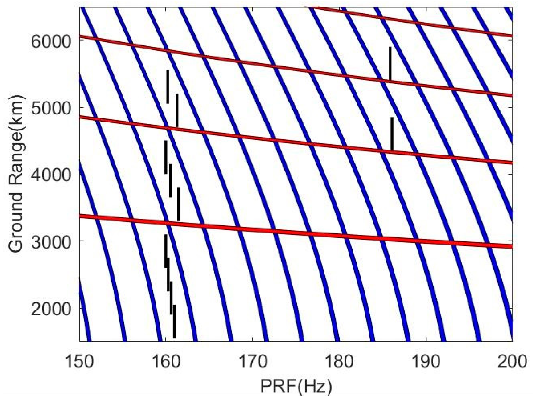
2.3. Doppler Bandwidth and PRF Analysis

The azimuth bandwidth of GEO-SA-BiSAR can be written as
B = | ( k 2 T λ 4 π + k R ) | T
with
k R = v R 2 λ R 0
where T is the illumination time for a point target in GEO-SA-BiSAR. With the parameters listed in Table 1, the azimuth bandwidth corresponding to the airborne multichannel receiver is 337.5 Hz, the Doppler bandwidth determined by the GEO transmitter is only 1.1 Hz (inclination is 60°), and the adopted synthetic aperture time is assumed to be 4.5 s.
The timing diagram selection result of the GEO SAR system for the swath coverage of 500 km is shown in Figure 2. The blue and red areas indicate the interference areas caused by nadir echoes and transmitted pulses, respectively, while these areas must be avoided during the timing diagram design. Generally speaking, because of the narrow instantaneous processed azimuth beam bandwidth of GEO monostatic SAR, the operating PRF in GEO monostatic SAR systems is usually less than 200 Hz in order to obtain the wide swath GEO SAR raw data with azimuth unambiguous sampling [29,30]. To obtain the desired area with 500 km ground range swath width, selected PRFs are indicated by the regions with black lines as shown in Figure 2, and the values of the selected PRF are in the range of 160–200 Hz. Therefore, the selected PRF value for the following SAR data simulation is set to 180 Hz.
According to the above analysis, the exploited azimuth bandwidth of the GEO-SA-BiSAR system is 338.6 Hz and larger than the adopted system PRF. Consequently, Doppler spectrum aliasing would occur as a result of the contradiction between the wider Doppler bandwidth because of the receiver velocity and the lower operating PRF in GEO SAR. In order to overcome the contradiction and resolve the Doppler spectrum aliasing, the azimuth multichannel receiving technology can be applied on the receiver platform. According to the principle of azimuth multichannel SAR [31,32], the total effective azimuth sampling rate with M azimuth channels can be increased to M PRF . Although just two azimuth receiving channels are needed in the airborne platform, three azimuth receiving channels are designed for a higher azimuth over-sampling rate in order to obtain a better Doppler spectrum ambiguity suppression effect.

3. Effects of the Target Velocity on Imaging Results

In the azimuth multichannel GEO-SA-BiSAR system, the different range history of the moving target causes the different multichannel impulse response in (23) with azimuth time delay and phase shift. To analyze the effects of the target velocity on these parameters in detail, designed simulation experiments are implemented, and Table 1 lists the corresponding simulation parameters.

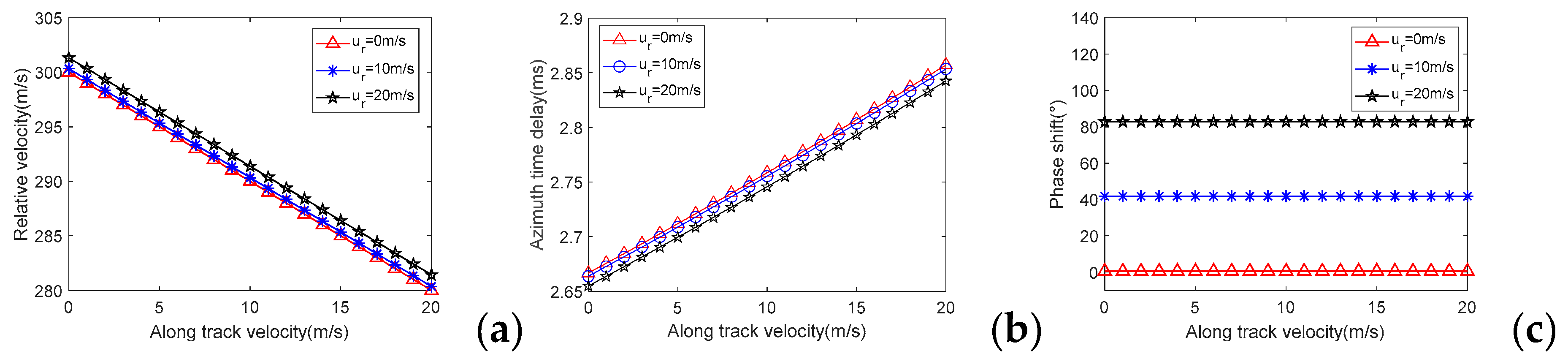
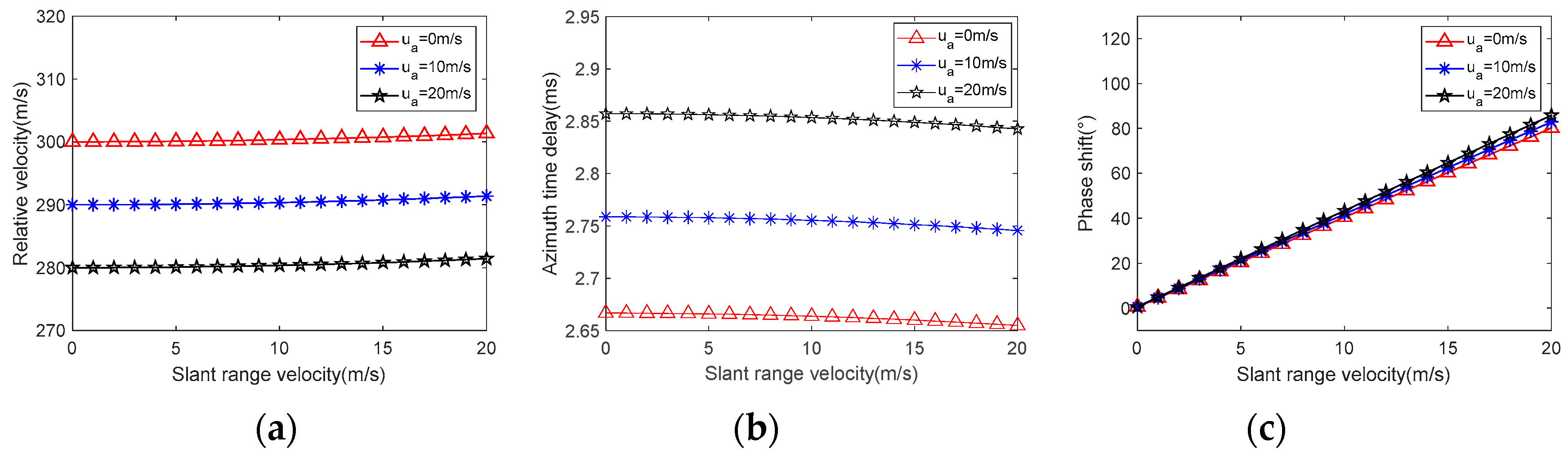
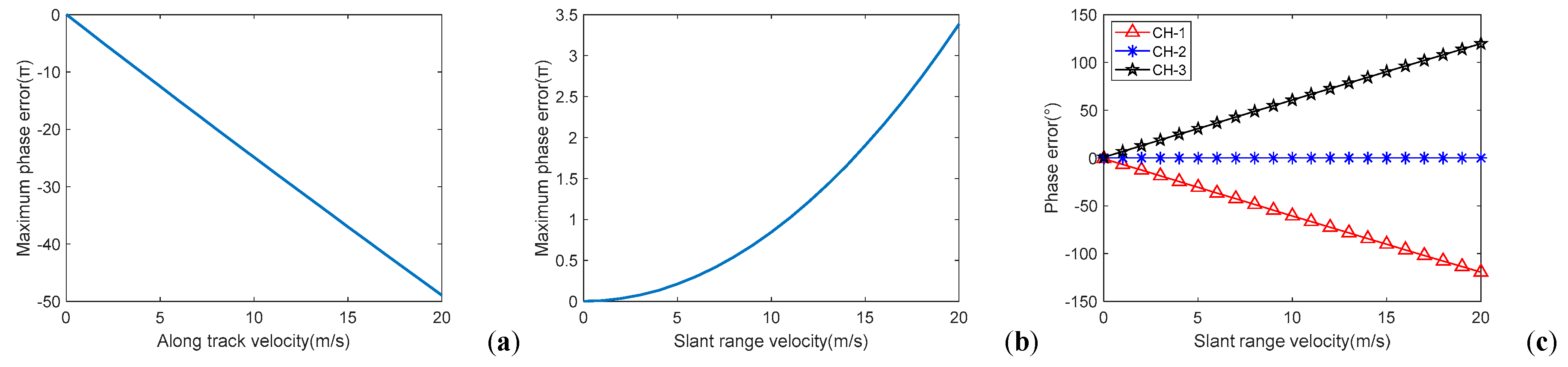
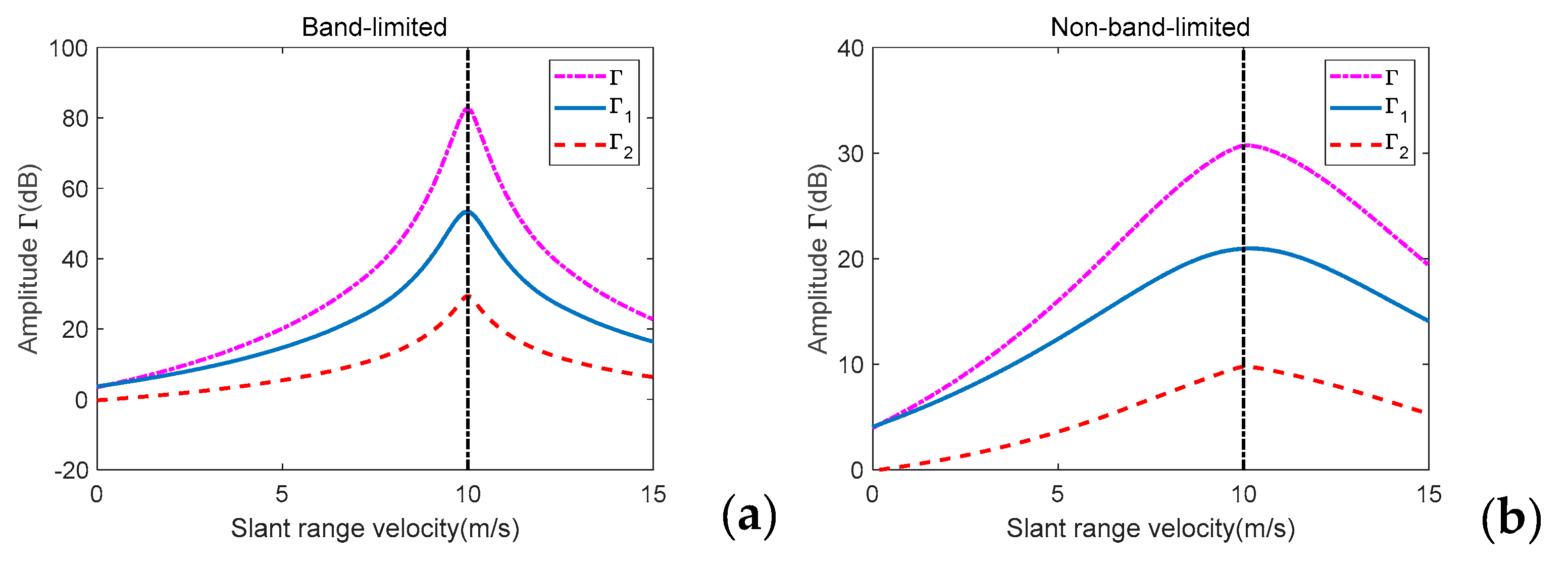
3.1. Effects on the Azimuth Multichannel Response

Figure 3 shows the influences of the along track velocity component on the three parameters aforementioned. The relative sensor velocity and azimuth time delay are sensitive to the along track velocity, but the phase shift is independent of the along track velocity. In Figure 3a, the relative sensor velocity varies from approximately 300 m/s to 280 m/s as the along track velocity changes. The influence of the along track velocity on the azimuth time delay is shown in Figure 3b, and the variation of the azimuth time delay with the change of the along track velocity is responsible for the changed phase function for azimuth multichannel reconstruction. In Figure 3c, the phase shift is independent of the along track velocity. In the previous simulation in Figure 3 to present the azimuth time delay and the phase shift varying with the along track velocity, parameters of the third channel are calculated, while the middle azimuth channel is considered as the reference channel.
In contrast with the effects of the azimuth velocity component, the phase shift is sensitive to the slant range velocity component, whereas the relative sensor velocity and the azimuth time delay are independent of the slant range velocity, as shown in Figure 4. The slant range velocity has an obviously lower impact on the relative sensor velocity and the azimuth time delay as shown in Figure 4a,b, and the influence on the relative sensor velocity can even be neglected. Unfortunately, the slant range velocity component introduces an obviously additive phase shift shown in Figure 4c, and the phase shift would result in azimuth multichannel phase imbalance.

3.2. Effects on Imaging Results

To validate the above analysis, imaging simulation experiments on point targets are designed according to the parameters in Table 1. Figure 5 shows imaging results of the stationary target for comparison, while Figure 6 and Figure 7 show the simulation results of the designed moving targets with the along track velocity of 10 m/s and the slant range velocity of 10 m/s, respectively.
As shown in Figure 5, Figure 6 and Figure 7, both slant range and along track velocities lead to azimuth defocusing and false targets. However, the azimuth defocusing phenomenon due to the azimuth velocity component is much more serious, as shown in Figure 6c, while the level of false targets introduced by the slant range velocity is obviously higher, as shown in Figure 7d. With the same value, the along track velocity introduces a larger relative sensor velocity change, which results in the larger additional phase error responsible for azimuth defocusing as shown in Figure 8a. Meanwhile, Figure 8b shows the maximum azimuth mismatch phase error in the synthetic aperture time caused by the slant range velocity, which leads to azimuth defocusing. However, the formation mechanisms of false targets due to the azimuth and slant range velocity component are quite different. The reason for false targets caused by the azimuth velocity component is azimuth non-uniform sampling because of the changed azimuth relative velocity, whereas the reason for false targets introduced by the slant range velocity is azimuth multichannel phase imbalance as shown in Figure 8c, since the phase shift is sensitive to the along track velocity. Taking the azimuth middle channel as the reference, Figure 8c shows the azimuth multichannel phase imbalance phenomenon varying with the slant range velocity.
Besides azimuth defocusing and false targets, the slant range also leads to the moving target location shift as shown in Figure 7b,d, and the azimuth location shift is caused by the additional Doppler shift due to the slant range and the changed azimuth modulation rate. Similar to the conventional SAR, the azimuth location shift is computed as
Δ x = v R u r R 0 / ( v R u a ) 2
As simulation results shown in Figure 5, Figure 6, Figure 7 and Figure 8, the azimuth velocity component mainly causes target defocusing in azimuth because of the azimuth Doppler modulation rate mismatch, whereas the slant range velocity component mainly causes azimuth false targets because of azimuth multichannel phase imbalance.

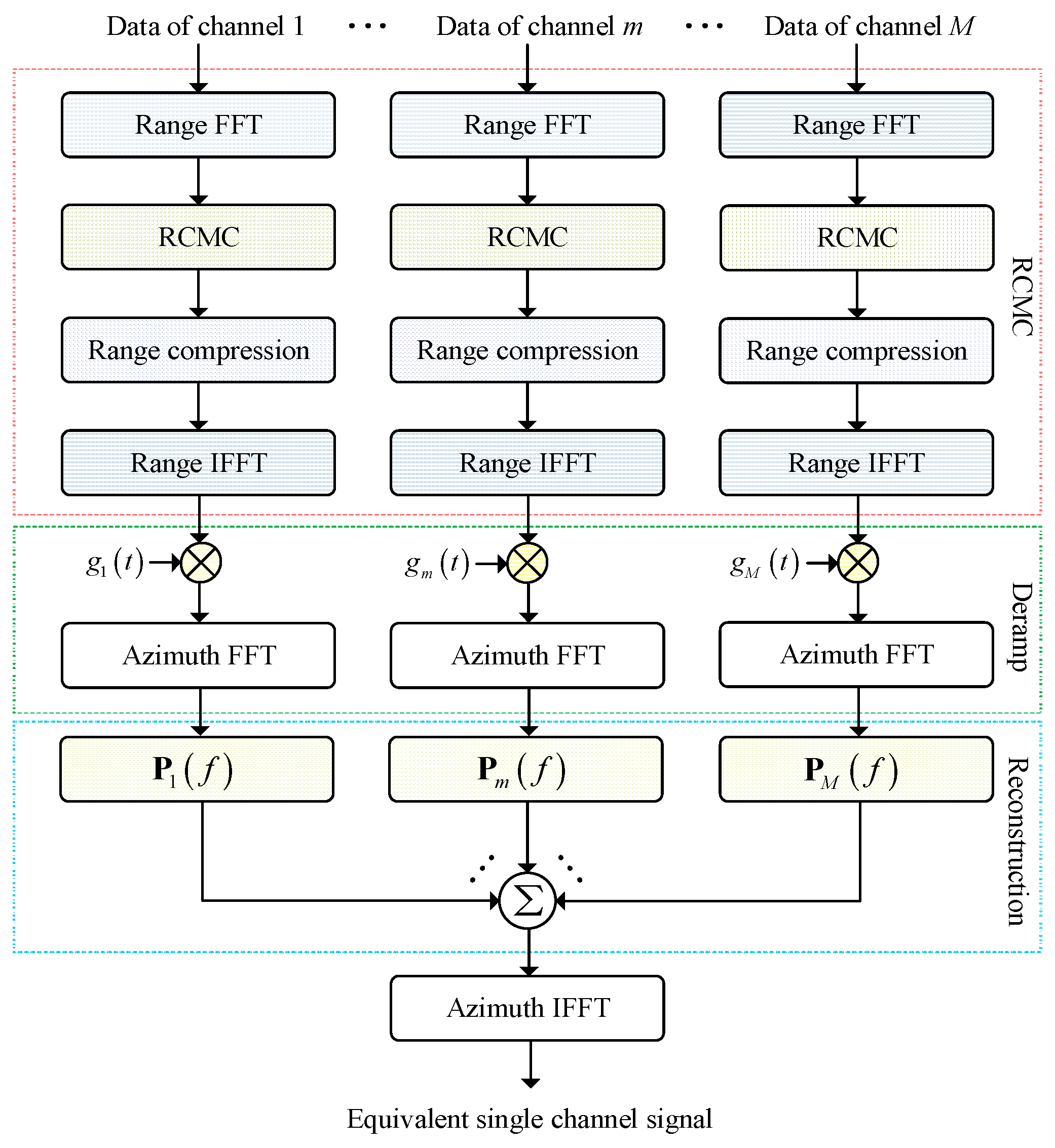
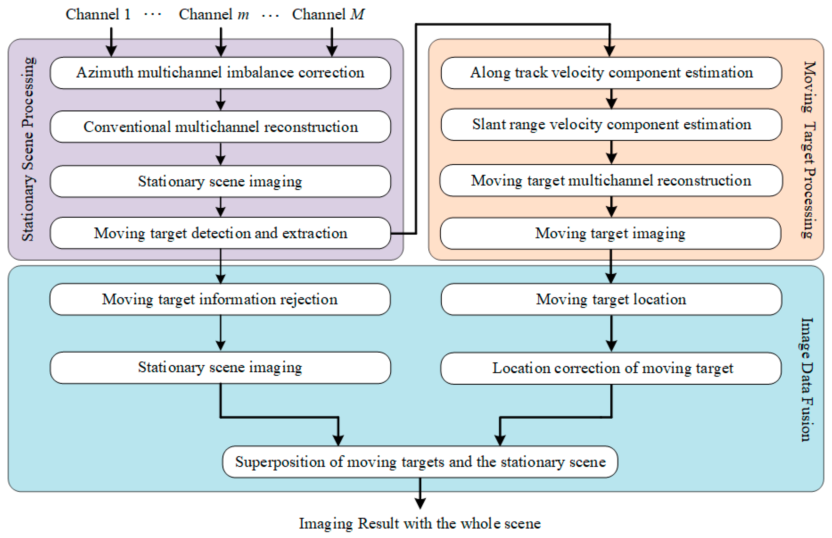
4. Azimuth Multichannel Reconstruction

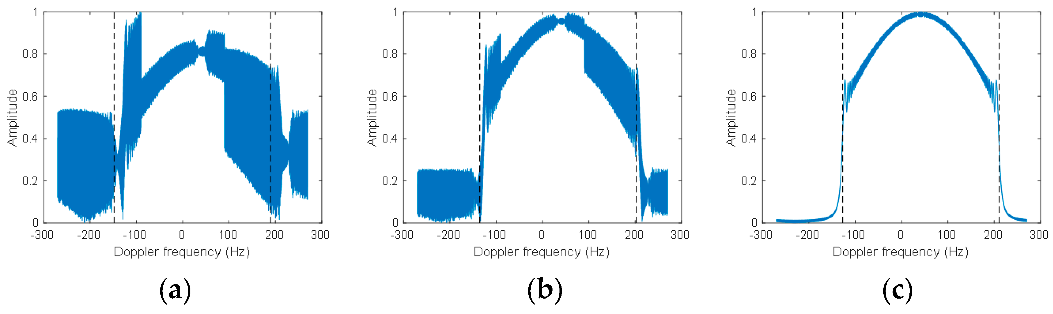
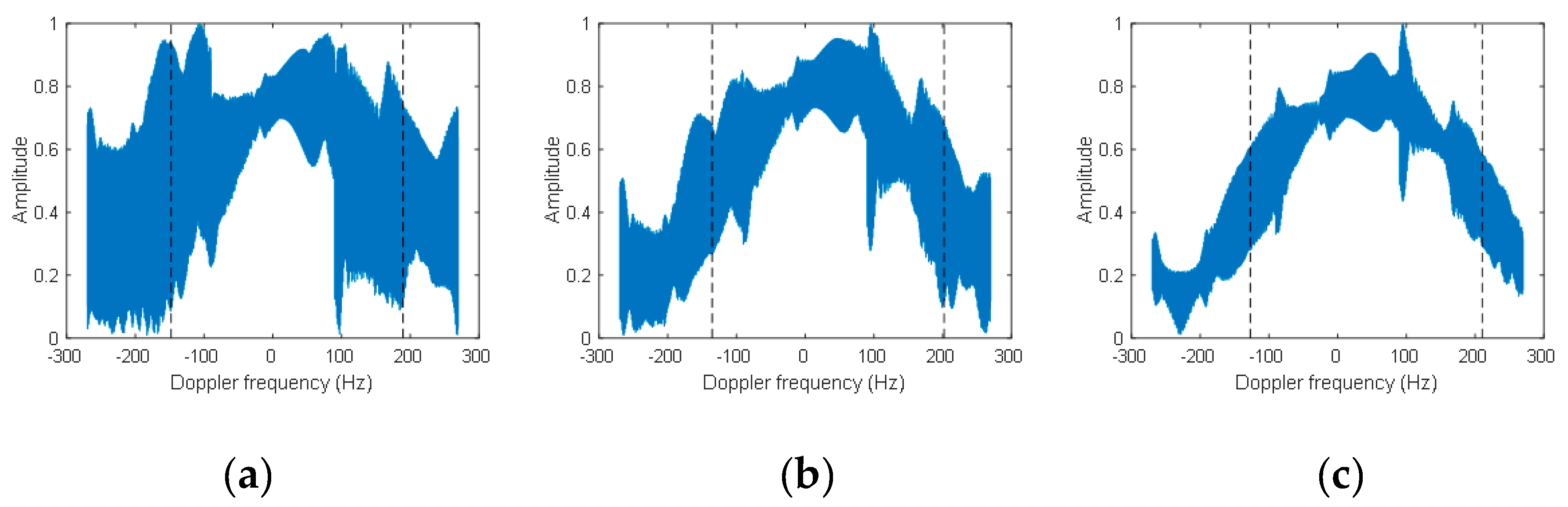
4.1. Azimuth Doppler Spectrum Reconstruction

As the above analysis indicates, the total effective azimuth Doppler sampling rate could be multiplied by arranging multiple receiving sub-apertures along the azimuth direction in a GEO-SA-BiSAR system. However, if the optimum PRF is not selected, additional azimuth multichannel reconstruction would be required to resolve the non-uniform sampling problem before the imaging processor. If the traditional azimuth multichannel reconstruction and imaging approaches were still adopted to process the echoes of moving targets, as shown in Figure 6 and Figure 7, imaging quality would be seriously reduced. Therefore, an innovative reconstruction approach based on the moving target azimuth multichannel response in (23) is proposed. Before combining azimuth multichannel raw data together, spatial-variant RCMC is performed to reduce the effects of the range cell migration on multichannel reconstruction and the Doppler bandwidth of the whole raw data is reduced by ANLCS. The key point of this approach is the azimuth multichannel reconstruction filters with the estimated velocity of the moving target. After the modified azimuth multichannel reconstruction, the moving target could be well focused, and its corresponding false targets could be obviously suppressed. The flowchart of the presented multichannel reconstruction approach is shown in Figure 9, and it includes three major processing steps: RCMC, azimuth de-ramping, and azimuth multichannel raw data combination.
Compared with the large stationary scene, the moving target is always of a small size, and its corresponding echoes are submerged in reflected echoes of the large stationary scene. After range compression, spatial-variant RCMC should be applied to reduce the effects of range cell migration (RCM) before azimuth multichannel reconstruction. The spatial-variant RCMC in GEO-SA-BiSAR could be achieved via keystone transform, and its detailed processing steps can be found in [25,33].
Furthermore, the instantaneous Doppler centroid varies with both the slant range and the azimuth location of the GEO transmitting platform, which extends the Doppler bandwidth of the raw data. Therefore, the varied instantaneous Doppler centroid should be removed before azimuth multichannel reconstruction by ANLCS, and ANLCS is implemented by multiplying the raw data by g m ( t )
g m ( t ) =   exp { j π [ q 2 ( t Δ x m v e ) 2 + q 3 ( t Δ x m v e ) 3 ] } exp { j π q 4 ( t Δ x m v e ) 4 }
where q i ( i = 2 , 3 , 4 ) are the coefficients of the ANLCS operation [24].
Transforming the multichannel impulse response of the moving target in (23) into the azimuth frequency domain, the multichannel impulse Doppler response S s , m ( f ) could be expressed as the product of the single channel GEO-SA-BiSAR impulse response S s ( f ) and the azimuth multichannel response function H m ( f ) as follows:
S s , m ( f ) S s ( f ) H m ( f )
with
S s ( f ) = FFT ( s s ( t ) )
H m ( f ) =   exp { j 2 π λ [ 1 2 R 0 ( Δ x m 2   v r v Δ x m 2 + 2 R 0 u r Δ x m v e ) ] } exp { j 2 π λ k 1 T Δ x m v e } exp { j 2 π Δ x m v e f }
where f represents the Doppler frequency. Consequently, the azimuth multichannel system matrix for the moving target in GEO-SA-BiSAR is given as follows:
H ( f ) = [ H 1 ( f ) H M ( f ) H 1 ( f + PRF ) H M ( f + PRF ) H 1 ( f + ( N 1 ) PRF ) H M ( f + ( N 1 ) PRF ) ]
Afterward, the azimuth multichannel reconstruction function P ( f ) is expressed as
P ( f ) = H 1 ( f )
The reconstruction function P ( f ) is a N × N matrix, while the reconstruction filter P n ( f ) for the n-th receiving channel consists of N filters. The entire Doppler frequency band I = [ N PRF / 2 , N PRF / 2 ] is divided into N sub-bands, and each channel is with a Doppler frequency centroid of f 0 , n = [ n ( N + 1 ) / 2 ] PRF . Afterward, the unambiguous spectrum of the imaged moving targets could be obtained by combining the echoes from all azimuth receiving channels. Finally, the equivalent raw data received by a single channel are obtained after azimuth inverse fast Fourier transform (IFFT).

4.2. Moving Target Velocity Estimation

According to (34), the azimuth multichannel reconstruction matrix in (36) for the imaged moving target is obtained from the given target velocity components in both directions. Therefore, the moving target velocity estimation is very important for azimuth multichannel reconstruction. As the relative sensor velocity change is mainly related to the along track velocity component, this component can be predicted by azimuth auto-focusing just like in the traditional case. However, for each azimuth channel, the azimuth signal is under-sampled and its corresponding spectrum is aliased, and the slant velocity cannot be obtained via the conventional Doppler centroid estimation approach.
With the system parameters listed in Table 1, both Figure 10 and Figure 11 show the azimuth multichannel reconstructed simulation results with different estimated slant range velocities when the designed slant range velocity is 10 m/s. Figure 10 shows the azimuth band-limited case, in which only the exploited azimuth beam width is considered, while Figure 11 shows the non-band-limited case, in which both in-band and out-of-band azimuth signals are considered during echo simulation of moving targets. In both cases, for the well reconstructed Doppler spectra with the accurate slant velocity, most signal power would gather around the estimated Doppler centroid as shown in Figure 10 and Figure 11.
According to the signal power distribution phenomenon shown in Figure 10 and Figure 11, the SIR could be introduced to judge whether the multichannel spectrum is well reconstructed. Furthermore, the SIR could be expressed as two types as follows:
Γ 1 ( u ^ r ) = B a / 2 + f ^ d c B a / 2 + f ^ d c W 2 ( f ; u ^ r ) d f N PRF / 2 + f ^ d c N PRF / 2 + f ^ d c W 2 ( f ; u ^ r ) d f B a / 2 + f ^ d c B a / 2 + f ^ d c W 2 ( f ; u ^ r ) d f
Γ 2 ( u ^ r ) = N PRF B a B a B a / 2 + f ^ d c B a / 2 + f ^ d c | W ( f ; u ^ r ) | d f N PRF / 2 + f ^ d c N PRF / 2 + f ^ d c | W ( f ; u ^ r ) | d f B a / 2 + f ^ d c B a / 2 + f ^ d c | W ( f ; u ^ r ) | d f
with
f ^ d c = u ^ r λ
where B a is the processed Doppler bandwidth, W ( f ; u ^ r ) indicates the reconstructed Doppler spectrum, and u ^ r is the estimated slant range velocity. The SIR Γ 1 represents the power ratio between in-band and out-of-band data, while the SIR Γ 2 indicates the average amplitude ratio between in-band and out-of-band data. To improve the slant range velocity estimation accuracy, the product Γ = Γ 1 Γ 2 of these two ratio parameters is used to estimate.
The introduced SIR Γ varying with the estimated slant range velocity is shown in Figure 12, and all SIRs reach the maximum value only when the accurate slant range velocity is adopted for azimuth multichannel reconstruction. Furthermore, the curve of Γ is the steepest among the three curves, which would result in the most accurate velocity estimation result. From Figure 12, it can be found that SIR Γ can well estimate the velocity of the moving target in both cases of band-limited and non-band-limited.
As we know, the moving target velocity estimation accuracy is mainly affected by the signal-to-clutter-and-noise ratio (SCNR) and ambiguity-to-signal ratio (ASR) levels, since echoes of the moving target are mixed with its corresponding ambiguity signal and echoes of the stationary scene in the receiving window. For SAR systems with airborne receivers, only azimuth ambiguity energy should be considered, and a higher operating PRF will obtain a lower ASR level. Consequently, to evaluate the accuracy of the presented velocity estimation approach based on the introduced SIR Γ , two sets of experiments on point targets are carried out. One is carried out to estimate the moving target slant range velocity under different SCNRs and selected PRF values, and the other is designed for different velocity estimations with the same SCNR and PRF. An L-band SAR image of the ocean is used to simulate the clutter signal, which is added to the simulated raw data of the moving target to obtain different SCNRs. In the first group of simulation experiments, the designed slant range velocity is set to 10 m/s. The velocity estimation results under different SCNRs and selected PRF values are obtained and summarized in Table 2. As shown in Table 2, the higher SCNR and PRF are with, the more accurate velocity estimation result would be achieved. Compared with the cases with different SCNRs, the effects of different PRF values are very small and can even be neglected, since all selected PRF values in Table 2 have a high azimuth over-sampling rate, which results in a low ASR level. To obtain the relative estimation error below 5%, the SCNR level should be greater than −10 dB. Therefore, clutter suppression should be carried out before the slant range velocity estimation, and the SCNR usually would be more than 0 dB after clutter suppression. As several clutter suppression methods in HRWS SAR have been proposed in recent years [34,35,36], clutter suppression will not be discussed in this paper. For simulation experiments in Table 3, the moving target is designed with the same SCNR but different slant range velocities. The simulated SCNR is set to −10 dB, and the estimated velocities are summerized in Table 3. As shown in Table 3, all deviations between the designed and estimated slant range velocities are below 0.15 m/s, and all relative errors are below 3%. The largest relative error of the estimation result is the sixth target, because the designed slant range velocity of the sixth moving target is too small at 1 m/s.

4.3. Moving Target Imaging in GEO-SA-BiSAR

In the real SAR raw data, echoes of the moving target are mixed with echoes of the stationary scene. Since the stationary target and the moving target have different Doppler characteristics and range cell migrations (RCMs) in azimuth multichannel GEO-SA-BiSAR, azimuth multichannel reconstruction and two-dimension (2D) focusing for the stationary scene and the moving target should be carried out separately. Therefore, the proposed imaging approach for moving targets in azimuth multichannel GEO-SA-BiSAR is shown in Figure 13, and the proposed imaging approach consists of three major parts: stationary scene processing, moving target processing, and image data fusion.
Azimuth multichannel imbalance, including amplitude, phase, and time delay, would seriously reduce the imaging quality, so multichannel imbalance correction should be carried out before azimuth multichannel reconstruction. Afterward, azimuth multichannel reconstruction and 2D focusing approaches suitable for azimuth multichannel GEO-SA-BiSAR in [24] should be performed. According to the aforementioned analysis and simulation results, the along track velocity component mainly leads to defocusing in azimuth, while the slant range velocity mainly results in false targets. Besides recently proposed moving target detection approaches [37], we could use this phenomenon to detect the moving target, especially for ocean scenes. After azimuth multichannel reconstruction and clutter suppression via Doppler filtering, moving targets can be detected in the obtain SAR image from the conventional imaging processor, and their corresponding positions can be approximately obtained. Since echoes of these moving targets are compressed in very limited range samples after range compression and RCMC, echoes of moving targets with very limited samples in both azimuth and range directions around their approximate position are extracted in the range azimuth-time domain before azimuth focusing. After extracting the echoes of these detected moving targets, the data of the corresponding areas is set to zero, and then echoes of the stationary scene is obtained after inverse focusing operation. Consequently, echoes of the stationary scene and moving targets could be processed separately. If different moving targets are far enough to each other, the echoes of these moving targets can be extracted and processed separately. However, the echoes of moving targets cannot be extracted individually, if they are too close to each other. In this case, the speed of one moving target or the average speed of multiple closely distributed moving targets can be used for imaging, at the cost of the imaging quality. But in practice, moving targets in the ocean scene usually will not be too close, unless they move together with almost the same speed.
In terms of processing extracted echoes of moving targets, both velocity components of moving targets should be alternately estimated at first. The along track velocity is estimated by azimuth auto-focusing, while the SIR Γ is introduced for the slant range velocity estimation. With the accurately estimated target velocity, azimuth multichannel echoes of the moving target could be well reconstruction. Finally, the reconstructed azimuth multichannel raw data of the moving target could be easily handled by the single channel imaging processor of GEO-SA-BiSAR [38].
After removing echoes of moving targets from the whole raw data of the imaged scene, the stationary imaged scene should be focused again. With the estimated target velocity including both velocity components in the azimuth and range directions, the moving target location correction can be easily implemented according to (30). Finally, the superposition result of the focused stationary scene and moving target focusing result after location correction can be obtained. It is noticed that the echo location of the moving target in the whole SAR raw data is known during extracting the echo signal of the moving target. Therefore, it is only need to superimpose the focused moving target on the stationary scene according to its corresponding location.

5. Simulation Experiment

In this section, simulation experiments on both point and distributed targets are designed to evaluate the proposed processing approach, and simulation parameters are summarized in Table 1. The height of the GEO transmit platform is 36,500 km, and its corresponding velocity along the azimuth direction is 2200 m/s. The height of the airborne receiver platform with three azimuth receiving channels is 3 km, and its velocity is 300 m/s. The synthetic aperture time for this GEO-SA-BiSAR is about 4.5 s, and its corresponding Doppler bandwidth is about 337.5 Hz. Because of the transmitted PRF of 180 Hz, the Doppler spectrum in each azimuth channel is aliased.

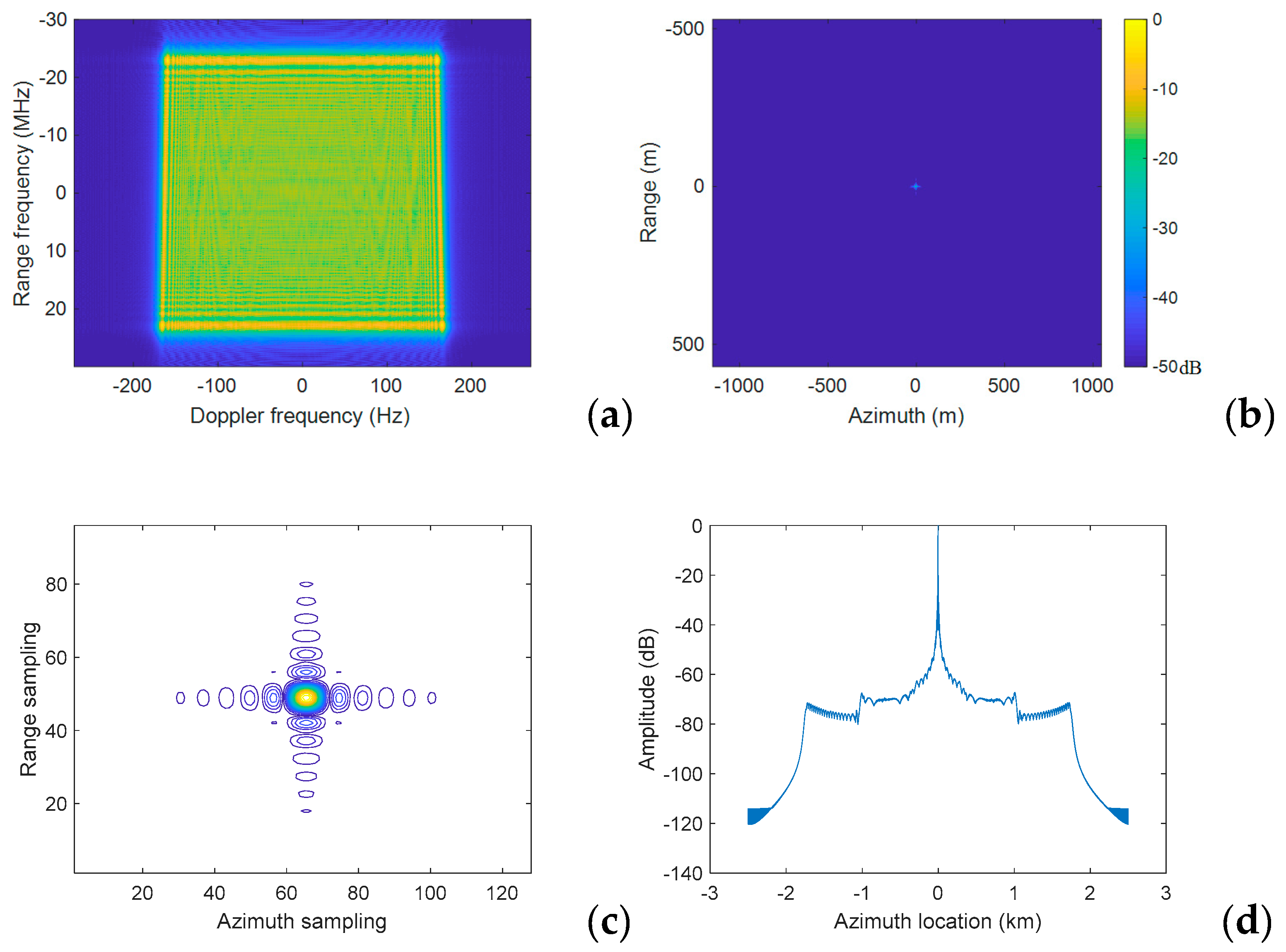
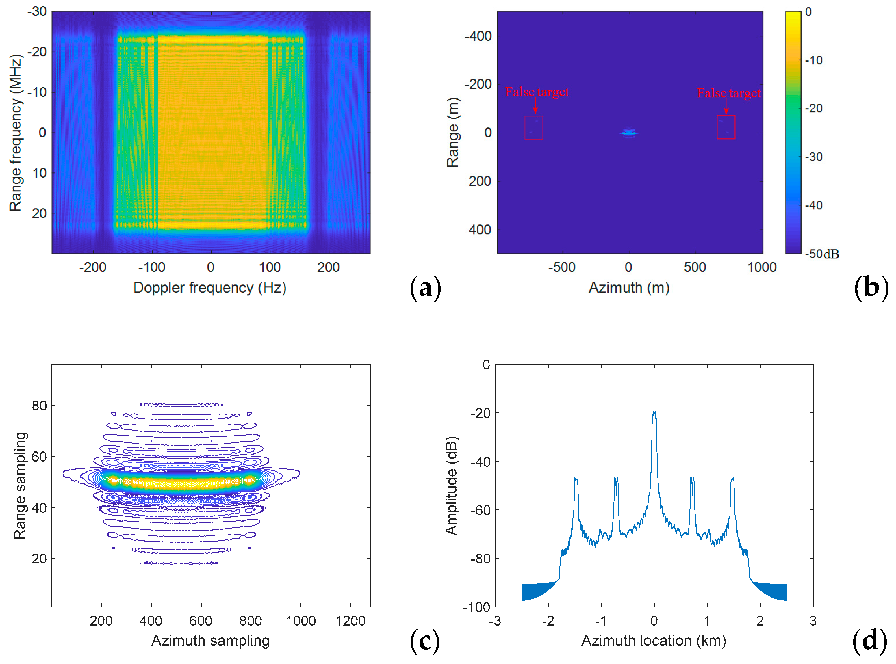
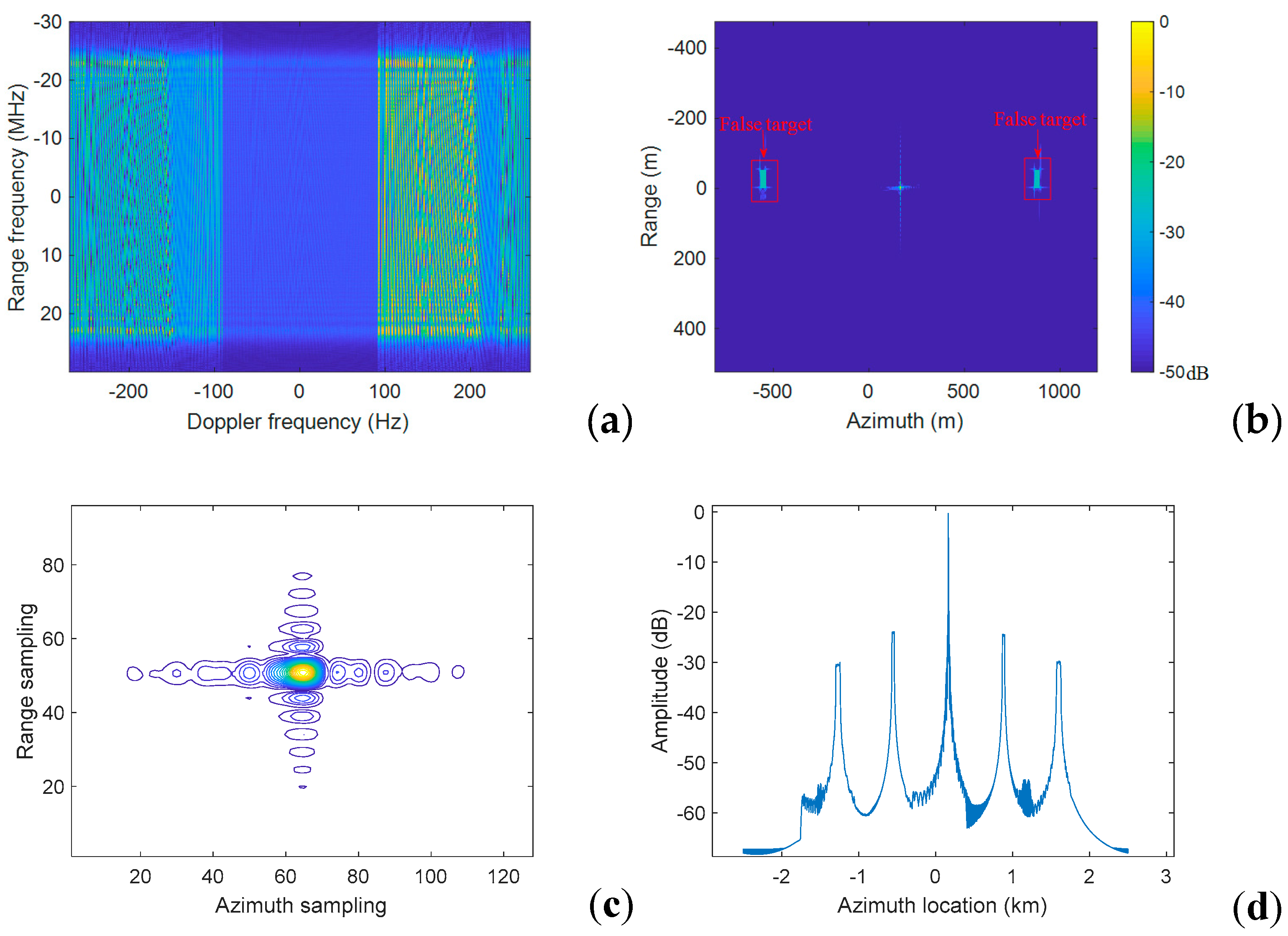
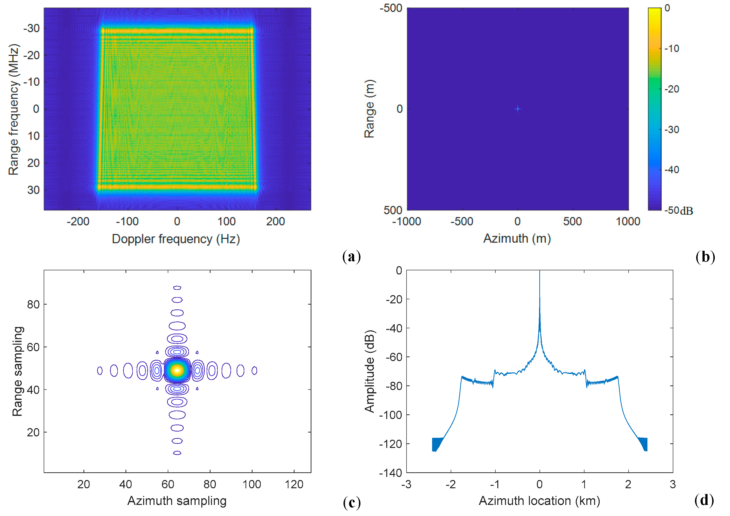
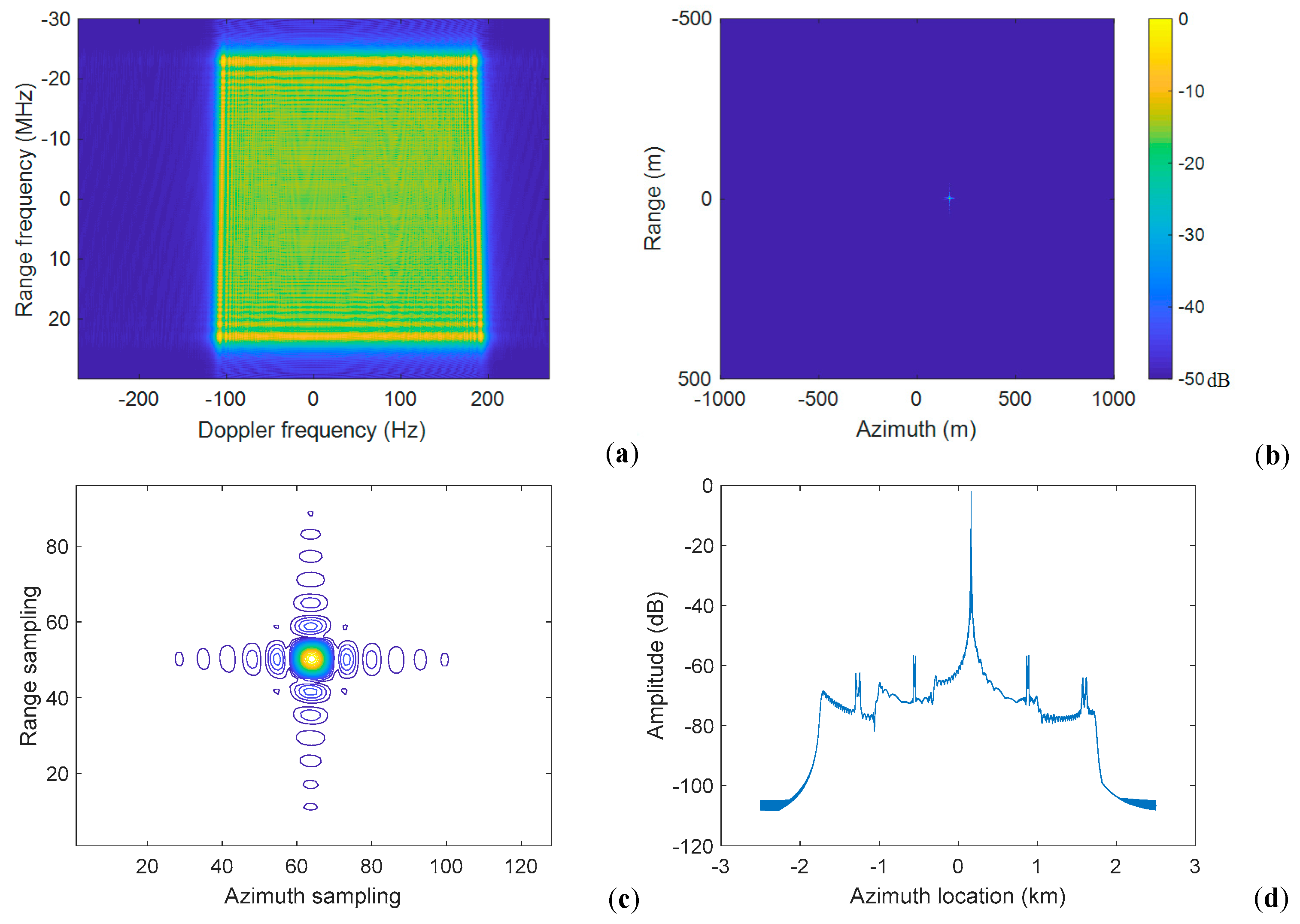
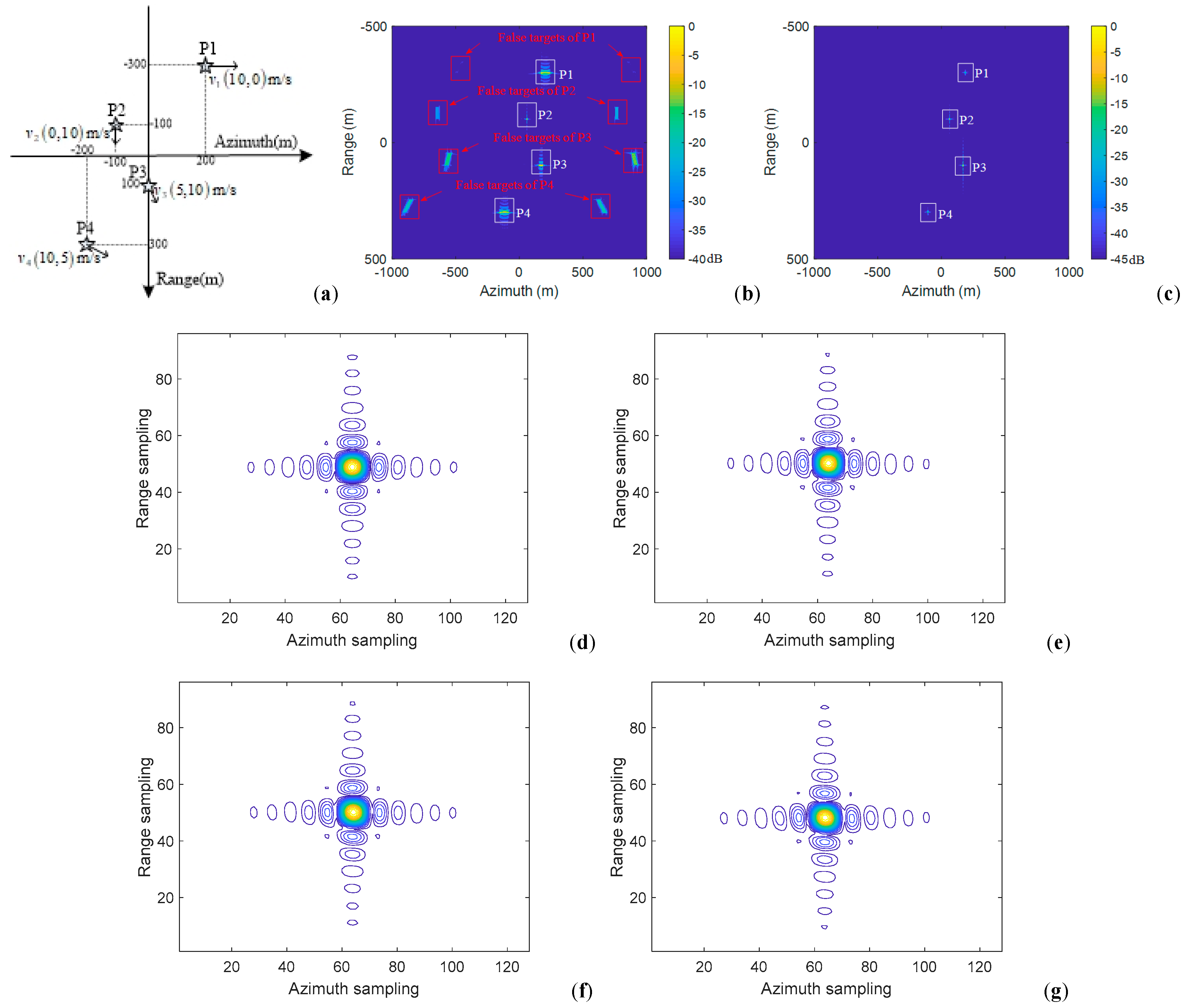
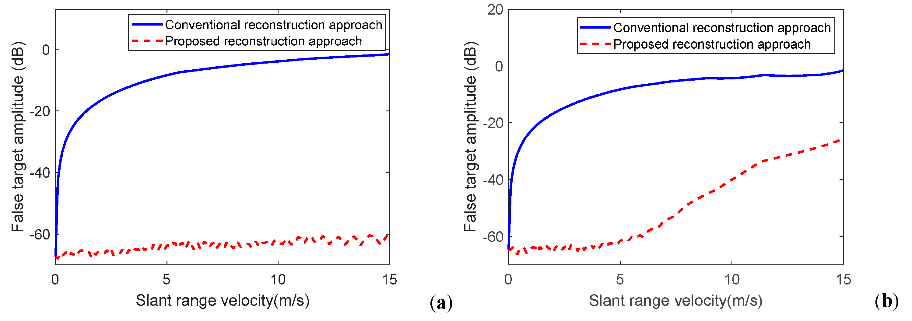
5.1. Simulation on Point Targets

First, two simulation experiments on a single moving target are carried out to demonstrate the proposed reconstruction approach. One single-point target is designed with only an along track velocity component of 10 m/s, and the other single-point target is designed with only a slant range velocity of 10 m/s. Their corresponding multichannel reconstruction and imaging results are shown in Figure 14 and Figure 15, respectively. Compared with the imaging results in Figure 6 and Figure 7, the imaging qualities are obviously improved as shown in Figure 14 and Figure 15, and their corresponding false targets are well suppressed as shown in Figure 14d and Figure 15d.
Furthermore, a simulation experiment on a designed scene with four point targets is carried out, and the relative geometrical relationship of the four point targets is shown in Figure 16a. All point targets have different moving velocities: target P1 has an along track velocity of 10 m/s, target P2 has a slant range velocity of 10 m/s, target P3 has an along track velocity of 5 m/s and a slant range velocity of 10 m/s, and target P4 has an along track velocity of 10 m/s and a slant range velocity of 5 m/s. With the conventional azimuth multichannel reconstruction approach, all point targets are defocused with obviously false targets as shown in Figure 16b. After adopting the proposed azimuth multichannel reconstruction and imaging approaches, the four targets are well focused and their false targets are obviously suppressed as shown in Figure 16c. Interpolated contour plots of the four points are shown in Figure 16d–g, it can be seen that each target is well focused, and their corresponding imaging quality parameters including resolution (res), integrated-side-lobe ratio (ISLR), peak-side-lobe ratio (PSLR) and maximum false target amplitude (MFTA) are measured and summarized in Table 4. Compared with the results obtained from the conventional imaging processor for the stationary scene and the theoretical values, the proposed approach shows better imaging capacity and false target suppression ability for moving targets.
Figure 17 shows the maximum false target amplitude by using the conventional and proposed approaches in both band-limited and non-band-limited cases. In the band-limited case, false targets are suppressed to below −60 dB and can be ignored. In the non-band-limited condition, false targets are suppressed to below −25 dB, the reduced amplitude level of false targets is less than the maximum azimuth ambiguity power in conventional SAR, and they almost would not affect following target detection and recognition.

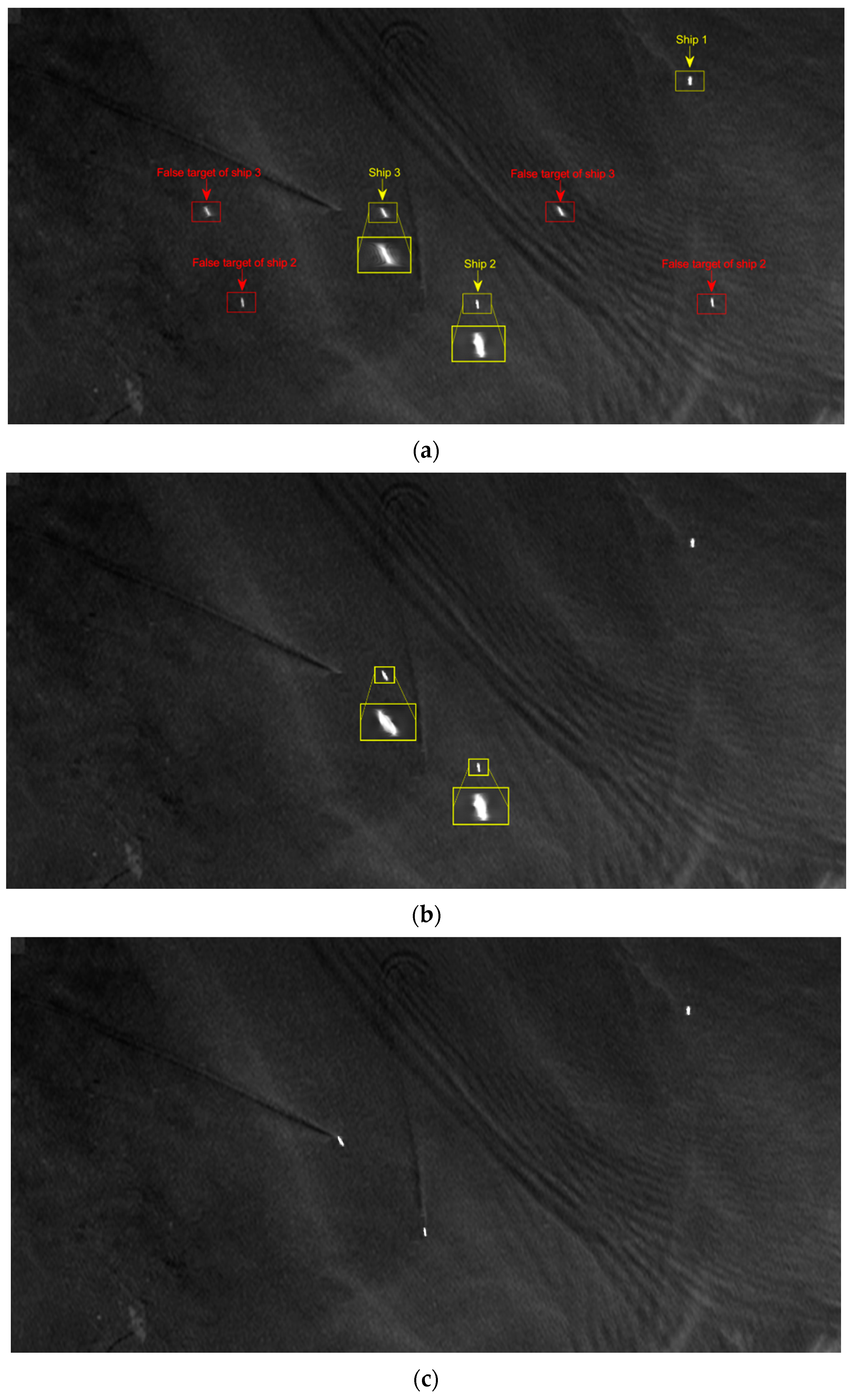
5.2. Simulation of Distributed Targets

To further evaluate the proposed multichannel reconstruction approach, a distributed ocean imaging scene simulation including three ships (denoted as ship 1, ship 2, and ship 3) is designed. The gray amplitude of a spaceborne ocean SAR image is set to be the input radar cross section (RCS) of the designed ocean, while the input RCSs of the three ships are also obtained from the real focused SAR image. The first ship is stationary and designed for comparison, the second ship moves along the slant range direction, and the third ship has both along track and slant range velocity components. The slant range velocity of ship 2 is 10 m/s, while both the along track and slant range velocity components of ship 3 are set to 10 m/s. The parameters of the multichannel GEO-SA-BiSAR system for this simulation experiment are listed in Table 1.
Figure 18a shows the imaging result after conventional azimuth multichannel reconstruction. Since ship 2 and ship 3 have slant range velocity components, their imaging result are with a pair of serious false targets and azimuth location shift. Furthermore, ship 3 is defocused in azimuth because of the along track velocity component. In Figure 18a, ship 2 and ship 3 have the same slant range velocity, but their corresponding distances between the real target and the adjacent false target are different. The reason for this phenomenon is that the distance is determined by both the slant range velocity and the slant range from the moving target to the airborne receiver. In Figure 18, the slant range of ship 2 and ship 3 are 6490 m and 4860 m, respectively, and their corresponding distances between the real target and the false target in theory are 934.58 m and 723.99 m, respectively. After measurement in Figure 18a, measured distances agree with the theoretical values. At the same time, according to (30), the resulting azimuth location shifts of ship 2 and ship 3 are also different, and their azimuth location shifts are 216.3 m and 167.6 m, respectively. Figure 18b shows the imaging result of the proposed azimuth multichannel reconstruction approach, the false targets of moving targets are well suppressed, while the defocused ship 3 in Figure 18a is well focused in Figure 18b. According to the location shift in (30), the moving target location can be corrected as shown in Figure 18c.

6. Conclusions

GEO-SA-BiSAR systems can obtain SAR images with finer azimuth resolution and higher SNR than monostatic GEO SAR systems with the same power consumption. However, the operating PRF of a GEO-SA-BiSAR system is less than the wide Doppler bandwidth determined by the airborne receiver, which leads to azimuth spectrum aliasing. In order to resolve this problem, azimuth multichannel technology is adopted in the airborne receiver platform in this study. Moreover, azimuth multichannel reconstruction of the echo signal is usually required, when the optimum PRF is not selected. In recent years, many researchers have studied conventional azimuth multichannel reconstruction approaches to address this problem.
However, because of the different Doppler modulation and range history between the stationary target and the moving target, the imaging geometry model of the moving target in GEO-SA-BiSAR is established in this paper. According to signal analysis and simulation results, the along track velocity mainly leads to target defocusing in azimuth, and the slant range velocity mainly results in false targets. To solve these problems, the novel multichannel reconstruction approach based on the azimuth multichannel response of the moving target is proposed, and the key point of the proposed approach is the modified multichannel reconstruction matrix corresponding to the estimated target velocity.
As the slant range velocity component of the imaged moving target should be known before azimuth multichannel reconstruction, a signal identity ratio between the in-band and out-of-band spectra is introduced for the slant range velocity estimation, and the velocity estimation accuracy is mainly determined by the SCNR. For ocean scenes with a high SCNR level, clutter suppression may not be required, but for most land scenes, clutter suppression must be performed before the slant range velocity estimation.

Author Contributions

Formal analysis, W.X.; methodology, W.X.; project administration, P.H. and B.L.; resources, P.H.; supervision, B.L.; visualization, Z.W.; writing—original draft, Z.W.; writing—review and editing, W.T., Z.G., and Y.D. All authors have read and agreed to the published version of the manuscript.

Funding

This work was supported in part by the National Equipment Pre-research Foundation of China under Grant Nos. JZX7Y20190253041401, JZX7Y20190253040501, and JZX7Y20190253040901, in part by the National Natural Science Foundation of China under Grant Nos. 61761037 and 61701264.

Conflicts of Interest

The authors declare no conflict of interest.

References

  1. Cumming, I.G.; Wong, F.H. Digital Processing of Synthetic Aperture Radar Data: Algorithms and Implementation; Artech House: Norwood, MA, USA, 2005. [Google Scholar]
  2. Tomiyasu, K. Synthetic aperture radar in geosynchronous orbit. In Proceedings of the 1978 Antennas and Propagation Society International Symposium, Washington, DC, USA, 15–19 March 1978. [Google Scholar]
  3. Tomiyasu, K. Conceptual Performance of a Satellite Borne, Wide Swath Synthetic Aperture Radar. IEEE Trans. Geosci. Remote Sens. 1981, 2, 108–116. [Google Scholar] [CrossRef]
  4. Tomiyasu, K. Tutorial review of synthetic-aperture radar (SAR) with applications to imaging of the ocean surface. Proc. IEEE 1978, 66, 563–583. [Google Scholar] [CrossRef]
  5. Tomiyasu, K.; Pacelli, J.L. Synthetic Aperture Radar Imaging from an Inclined Geosynchronous Orbit. IEEE Trans. Geosci. Remote Sens. 1983, 21, 324–329. [Google Scholar] [CrossRef]
  6. Moreira, A.; Prats Iraola, P.; Younis, M.; Krieger, G.; Hajnsek, I.; Papathanassiou, K.P. A tutorial on synthetic aperture radar. IEEE Geosci. Remote Sens. Mag. 2013, 1, 6–43. [Google Scholar] [CrossRef] [Green Version]
  7. Moreira, A.; Krieger, G.; Hajnsek, I. Tandem-L: A Highly Innovative Bistatic SAR Mission for Global Observation of Dynamic Processes on the Earth’s Surface. IEEE Geosci. Remote Sens. Mag. 2015, 3, 8–23. [Google Scholar] [CrossRef]
  8. Hu, C.; Long, T.; Zeng, T.; Liu, F.; Liu, Z. The Accurate Focusing and Resolution Analysis Method in Geosynchronous SAR. IEEE Trans. Geosci. Remote Sens. 2011, 49, 3548–3563. [Google Scholar] [CrossRef]
  9. Hobbs, S.; Mitchell, C.; Forte, B.; Holley, R.; Snapir, B.; Whittaker, P. System Design for Geosynchronous Synthetic Aperture Radar Missions. IEEE Trans. Geosci. Remote Sens. 2014, 52, 7750–7763. [Google Scholar] [CrossRef] [Green Version]
  10. Sun, Z.; Wu, J.; Pei, J.; Li, Z.; Huang, Y.; Yang, J. Inclined Geosynchronous Spaceborne–Airborne Bistatic SAR: Performance Analysis and Mission Design. IEEE Trans. Geosci. Remote Sens. 2016, 54, 343–357. [Google Scholar] [CrossRef]
  11. Wang, J.; Wang, Y.; Zhang, J.; Ge, J. Resolution Calculation and Analysis in Bistatic SAR With Geostationary Illuminator. IEEE Geosci. Remote Sens. Lett. 2013, 10, 194–198. [Google Scholar] [CrossRef]
  12. An, H.; Wu, J.; He, Z.; Li, Z.; Yang, J. Geosynchronous Spaceborne-Airborne Multichannel Bistatic SAR Imaging Using Weighted Fast Factorized Backprojection Method. IEEE Geosci. Remote Sens. Lett. 2019, 16, 1590–1594. [Google Scholar] [CrossRef]
  13. Wang, Y.; Liu, Y.; Li, Z.; Suo, Z.; Fang, C.; Chen, J. High-Resolution Wide-Swath Imaging of Spaceborne Multichannel Bistatic SAR with Inclined Geosynchronous Illuminator. IEEE Geosci. Remote Sens. Lett. 2017, 14, 2380–2384. [Google Scholar] [CrossRef]
  14. Wu, J.; Sun, Z.; An, H.; Qu, J.; Yang, J. Azimuth Signal Multichannel Reconstruction and Channel ConFigureuration Design for Geosynchronous Spaceborne–Airborne Bistatic SAR. IEEE Trans. Geosci. Remote Sens. 2019, 57, 1861–1872. [Google Scholar] [CrossRef]
  15. Lopez-Dekker, P.; Mallorqui, J.J.; Serra-Morales, P.; Sanz-Marcos, J. Phase Synchronization and Doppler Centroid Estimation in Fixed Receiver Bistatic SAR Systems. IEEE Trans. Geosci. Remote Sens. 2008, 46, 3459–3471. [Google Scholar] [CrossRef]
  16. Zeng, T.; Hu, C.; Wu, L.; Liu, F.; Tian, W.; Zhu, M.; Long, T. Extended NLCS Algorithm of BiSAR Systems With a Squinted Transmitter and a Fixed Receiver: Theory and Experimental Confirmation. IEEE Trans. Geosci. Remote Sens. 2013, 51, 5019–5030. [Google Scholar] [CrossRef]
  17. Anghel, A.; Cacoveanu, R.; Moldovan, A.; Rommen, B.; Datcu, M. COBIS: Opportunistic C-Band Bistatic SAR Differential Interferometry. IEEE J. Sel. Top. Appl. Earth Obs. Remote Sens. 2019, 12, 3980–3998. [Google Scholar] [CrossRef]
  18. Baumgartner, S.V.; Krieger, G. Simultaneous High-Resolution Wide-Swath SAR Imaging and Ground Moving Target Indication: Processing Approaches and System Concepts. IEEE J. Sel. Top. Appl. Earth Obs. Remote Sens. 2015, 8, 5015–5029. [Google Scholar] [CrossRef]
  19. Gebert, N.; Krieger, G. Azimuth Phase Center Adaptation on Transmit for High-Resolution Wide-Swath SAR Imaging. IEEE Geosci. Remote Sens. Lett. 2009, 6, 782–786. [Google Scholar] [CrossRef]
  20. Huang, P.; Li, S.; Xu, W. Investigation on Full-Aperture Multichannel Azimuth Data Processing in TOPS. IEEE Geosci. Remote Sens. Lett. 2014, 11, 728–732. [Google Scholar] [CrossRef]
  21. Xu, W.; Huang, P.; Wang, R.; Deng, Y. Processing of Multichannel Sliding Spotlight and TOPS Synthetic Aperture Radar Data. IEEE Trans. Geosci. Remote Sens. 2013, 51, 4417–4429. [Google Scholar] [CrossRef]
  22. Xu, W.; Huang, P.; Tan, W. Azimuth Phase Coding by Up and Down Chirp Modulation for Range Ambiguity Suppression. IEEE Access 2019, 7, 143780–143791. [Google Scholar] [CrossRef]
  23. Xu, W.; Hu, J.; Huang, P.; Tan, W.; Dong, Y. Azimuth Phase Center Adaptive Adjustment upon Reception for High-Resolution Wide-Swath Imaging. Sensors 2019, 19, 4277. [Google Scholar] [CrossRef] [PubMed] [Green Version]
  24. An, H.; Wu, J.; Sun, Z.; Yang, J. A Two-Step Nonlinear Chirp Scaling Method for Multichannel GEO Spaceborne–Airborne Bistatic SAR Spectrum Reconstructing and Focusing. IEEE Trans. Geosci. Remote Sens. 2019, 57, 3713–3728. [Google Scholar] [CrossRef]
  25. Wu, J.; Sun, Z.; Li, Z.; Huang, Y.; Yang, J.; Liu, Z. Focusing translational variant bistatic forward-looking SAR using keystone transform and extended nonlinear chirp scaling. Remote Sens. 2016, 8, 840. [Google Scholar] [CrossRef] [Green Version]
  26. Tan, W.; Xu, W.; Huang, P.; Huang, Z.; Qi, Y.; Han, K. Investigation of Azimuth Multichannel Reconstruction for Moving Targets in High Resolution Wide Swath SAR. Sensors 2017, 17, 1270–1282. [Google Scholar] [CrossRef] [Green Version]
  27. Li, Z.; Wu, J.; Yi, Q.; Huang, Y.; Yang, J.; Bao, Y. Bistatic Forward-Looking SAR Ground Moving Target Detection and Imaging. IEEE Trans. Aerosp. Electron. Syst. 2015, 51, 1000–1016. [Google Scholar] [CrossRef]
  28. Zhao, B.; Qi, X.; Deng, Y.; Wang, R.; Song, H. Accurate fourth-order doppler parameter estimation approach for geosynchronous SAR. In Proceedings of the EUSAR 2012; 9th European Conference on Synthetic Aperture Radar, Nuremberg, Germany, 24–26 April 2012. [Google Scholar]
  29. Ruiz-Rodon, J.; Broquetas, A.; Makhoul, E.; Guarnieri, A.M.; Rocca, F. Nearly Zero Inclination Geosynchronous SAR Mission Analysis With Long Integration Time for Earth Observation. IEEE Trans. Geosci. Remote Sens. 2014, 52, 6379–6391. [Google Scholar] [CrossRef]
  30. Ding, Z.; Shu, B.; Yin, W.; Zeng, T.; Long, T. A Modified Frequency Domain Algorithm Based on Optimal Azimuth Quadratic Factor Compensation for Geosynchronous SAR Imaging. IEEE J. Sel. Top. Appl. Earth Obs. Remote Sens. 2016, 9, 1119–1131. [Google Scholar] [CrossRef]
  31. Papoulis, A. Generalized sampling expansion. IEEE Trans. Circuits Syst. 1977, 24, 652–654. [Google Scholar] [CrossRef]
  32. Gebert, N.; Villano, M.; Krieger, G.; Moreira, A. Multichannel Azimuth Processing in ScanSAR and TOPS Mode Operation. IEEE Trans. Geosci. Remote Sens. 2013, 51, 4611. [Google Scholar] [CrossRef]
  33. Wu, J.; Li, Z.; Huang, Y.; Yang, J.; Yang, H.; Liu, Q.H. Focusing Bistatic Forward-Looking SAR With Stationary Transmitter Based on Keystone Transform and Nonlinear Chirp Scaling. IEEE Geosci. Remote Sens. Lett. 2014, 11, 148–152. [Google Scholar] [CrossRef]
  34. Sjogren, T.K.; Viet, T.V.; Pettersson, M.I. Suppression of Clutter in Multichannel SAR GMTI. IEEE Trans. Geosci. Remote Sens. 2014, 52, 4005–4013. [Google Scholar] [CrossRef]
  35. Yang, L.; Wang, T.; Xing, M.; Bao, Z. The Clutter Suppression Method of Airborne Multi-channel SAR-GMTI System. J. Electron. Inf. Technol. 2011, 30, 2831–2834. [Google Scholar] [CrossRef]
  36. Zhang, S.-X.; Xing, M.; Xia, X.-G.; Guo, R.; Liu, Y.-Y.; Bao, Z. Robust Clutter Suppression and Moving Target Imaging Approach for Multichannel in Azimuth High-Resolution and Wide-Swath Synthetic Aperture Radar. IEEE Trans. Geosci. Remote Sens. 2015, 53, 687–709. [Google Scholar] [CrossRef]
  37. Sun, H.-B.; Liu, G.-S.; Gu, H.; Su, W.-M. Application of the fractional Fourier transform to moving target detection in airborne SAR. IEEE Trans. Aerosp. Electron. Syst. 2002, 38, 1416–1424. [Google Scholar]
  38. Zhu, D.; Li, Y.; Zhu, Z. A Keystone Transform Without Interpolation for SAR Ground Moving-Target Imaging. IEEE Geosci. Remote Sens. Lett. 2007, 4, 18–22. [Google Scholar] [CrossRef]
Figure 1. The observation geometry in azimuth multichannel geosynchronous spaceborne–airborne bistatic synthetic aperture radar (GEO-SA-BiSAR).
Remotesensing 12 01703 g001
Figure 2. Timing diagram selection result of the monostatic geostationary synthetic aperture radar (GEO SAR) with a swath width of 500 km.
Remotesensing 12 01703 g002
Figure 3. Effects of the along track velocity on different azimuth multichannel parameters in the multichannel GEO-SA-BiSAR system. (a) Relative sensor velocity. (b) Azimuth time delay. (c) Phase shift.
Remotesensing 12 01703 g003
Figure 4. Effects of the slant range velocity on different azimuth multichannel parameters in the multichannel GEO-SA-BiSAR system. (a) Relative sensor velocity. (b) Azimuth time delay. (c) Phase shift.
Remotesensing 12 01703 g004
Figure 5. Imaging results of the stationary target in azimuth multichannel GEO-SA-BiSAR. (a) Reconstructed two-dimension spectrum. (b) The focused point target. (c) Contour plots of the point target. (d) The maximum azimuth projection profile.
Remotesensing 12 01703 g005
Figure 6. The focused moving target with the along track velocity of 10 m/s. (a) Reconstructed two-dimension spectrum. (b) The focused point target. (c) Contour plots of the point target. (d) The maximum azimuth projection profile.
Remotesensing 12 01703 g006
Figure 7. Simulation results of the moving target with the slant velocity of 10 m/s. (a) Reconstructed two-dimension spectrum. (b) The focused point target. (c) Contour plots of the point target. (d) The maximum azimuth projection profile.
Remotesensing 12 01703 g007
Figure 8. The influence of the velocity of the moving target. (a) The maximum phase error caused by the along track velocity. (b) The maximum phase error due to the slant range velocity. (c) Azimuth multichannel phase imbalance due to the slant range velocity.
Remotesensing 12 01703 g008
Figure 9. Flowchart of the proposed multichannel reconstruction approach.
Remotesensing 12 01703 g009
Figure 10. Reconstructed Doppler spectra via different slant range velocities for reconstruction in the band-limited case, while the actual target slant range velocity is 10 m/s. (a) The slant range velocity for reconstruction is 5 m/s. (b) The slant range velocity for reconstruction is 8 m/s. (c) The slant range velocity for reconstruction is 10 m/s.
Remotesensing 12 01703 g010
Figure 11. Reconstructed Doppler spectra via different slant range velocities for reconstruction in the non-band-limited case, while the actual target slant range velocity is 10 m/s. (a) The slant range velocity for reconstruction is 5 m/s. (b) The slant range velocity for reconstruction is 8 m/s. (c) The slant range velocity for reconstruction is 10 m/s.
Remotesensing 12 01703 g011
Figure 12. The introduced signal intensity ratios (SIRs) for the slant range velocity estimation. (a) The azimuth band-limited case. (b) The azimuth non-band-limited case.
Remotesensing 12 01703 g012
Figure 13. The flowchart of the proposed imaging approach for moving targets in azimuth multichannel GEO-SAR-BiSAR.
Remotesensing 12 01703 g013
Figure 14. The imaging result via the proposed approach when the along track velocity is 10 m/s. (a) Reconstructed two-dimension spectrum. (b) The focused point target. (c) Contour plots of the point target. (d) The maximum azimuth projection profile.
Remotesensing 12 01703 g014
Figure 15. The imaging result via the proposed approach when the slant range velocity is 10 m/s. (a) Reconstructed two-dimension spectrum. (b) The focused point target. (c) Contour plots of the point target. (d) The maximum azimuth projection profile.
Remotesensing 12 01703 g015
Figure 16. Imaging results of point targets. (a) Geometry of simulated point targets. (b) Conventional azimuth multichannel reconstruction. (c) Proposed azimuth multichannel reconstruction. Contour plots of targets 1–4. (d) Target P1. (e) Target P2. (f) Target P3. (g) Target P4.
Remotesensing 12 01703 g016
Figure 17. The relationship between the maximum false target amplitude with the different slant range velocities. (a) The azimuth band-limited case. (b) The azimuth non-band-limited case.
Remotesensing 12 01703 g017
Figure 18. Comparison of the imaging results of the designed distributed ocean scene. (a) Imaging result obtained from the conventional azimuth multichannel reconstruction approach. (b) Imaging result obtained from the proposed multichannel reconstruction approach. (c) Imaging result after location correction.
Remotesensing 12 01703 g018
Table 1. Designed parameters in GEO-SA-BiSAR for simulation.
ParameterValue
Center frequency1.25 GHz
PRF180 Hz
Pulse bandwidth50 MHz
Integration time4.5 s
Eccentricity0
Inclination60°
Right ascension of ascending node195.5°
Argument of perigee270°
Off nadir angle
Receiver height3 km
Slant range to scene center5 km
Receiver velocity300 m/s
Receiving channels3
Receive sub-aperture length0.8 m
Table 2. Slant-range velocity estimation results with different signal-to-clutter-and-noise ratios (SCNRs).
SCNR(dB)−50−40−30−20−10010
PRF = 170 HzEstimated velocity (m/s)14.9313.3712.3910.8510.4210.3310.23
Deviation (m/s)4.933.372.390.850.420.330.23
Relative error49.3%33.7%23.9%8.5%4.2%3.3%2.3%
PRF = 180 HzEstimated velocity (m/s)14.9514.3211.3310.5910.1910.1210.12
Deviation (m/s)4.954.321.330.590.190.120.12
Relative error49.5%43.2%13.3%5.9%1.9%1.2%1.2%
PRF = 190 HzEstimated velocity (m/s)15.685.278.0110.7310.1210.1110.04
Deviation (m/s)5.684.731.990.730.120.110.04
Relative error56.8%47.3%19.9%7.3%1.2%1.1%0.4%
Table 3. Slant-range velocity estimation results for different targets with the same SCNR.
Target Index12345678910
Velocity (m/s)−14−11−8−5−21471013
Estimated velocity (m/s)−14.19−11.11−7.91−5.12−1.891.154.157.1110.1713.14
Deviation (m/s)0.190.110.090.120.110.150.150.110.170.14
Relative error1.4%1.0%1.1%2.4%5.5%15%3.7%1.5%1.7%1.1%
Table 4. Imaging quality parameters on simulated point targets in multichannel GEO-SA-BiSAR.
MethodTargetAzimuthRangeMFTA
(dB)
Res(m)PSLR(dB)ISLR(dB)Res(m)PSLR(dB)ISLR(dB)
ConventionalP159.55−26.30−26.372.64−13.01−9.77−44.43
P21.06−11.26−7.652.70−13.46−10.19−21.95
P38.77−7.94−10.582.68−12.78−9.32−20.82
P417.99−5.10−4.152.66−13.25−9.86−25.04
ProposedP10.83−13.25−10.012.64−13.22−9.92−68.89
P20.80−13.07−10.142.69−13.48−10.19−56.68
P30.81−13.11−10.112.68−13.42−10.15−52.42
P40.83−13.26−10.092.67−13.34−10.07−47.56
Theoretical valueP10.81−13.26−9.802.66−13.26−9.80--
P20.79−13.26−9.802.66−13.26−9.80--
P30.80−13.26−9.802.66−13.26−9.80--
P40.81−13.26−9.802.66−13.26−9.80--

