1. Introduction
Recently, remote sensing has been used to continuously monitor and manage the ecological changes of plants in time and space [
1,
2]. Compared with basic measurement methods, remote sensing has the characteristics of real-time, dynamic, and large-scale and can obtain a large area of soil and crop information. Remote sensing is widely used in crop area, growth, yield estimation, and soil moisture monitoring [
3,
4,
5,
6,
7]. The Fraction of Absorbed Photosynthetically Active Radiation (FPAR) is the ratio of Photosynthetically Active Radiation (PAR) absorbed by the green part of the vegetation canopy to the total PAR at the top of the canopy [
8,
9]. The methods for estimating FPAR based on remote sensing mainly include the empirical statistical model and physical model. The empirical statistical model is widely used due to its simplicity, minimal parameters, and high computational efficiency. However, this model is less feasible than a more complex physical model, which involves more parameters inferred from the perspective of energy balance.
There are several global FPAR data sets, such as the Moderate Resolution Imaging Spectro Radiometer (MODIS), the Multi–angle Imaging Spectro Radiometer (MISR) FPAR, the Carbon Cycle and Change in Land Observational Products from an Ensemble of Satellites (CYCLOPES) FPAR, the Joint Research Center (JRC) FPAR, the Geoland Version1 (GEOV01) FPAR, the Global Land Surface Satellite (GLASS) FPAR, and so on [
9,
10,
11]. For example, Myneni et al. [
12,
13,
14] formed a MODIS global Leaf Area Index (LAI)/FPAR product (MOD15) based on a three-dimensional radiated transfer model and the Look-Up Table (LUT) algorithm from MODIS data. Baret et al. [
15] generated a GEOV01 global FPAR product based on a neural network from spot/vegetation data. Gobron et al. [
16] generated JRC-FPAR based on the continuous vegetation canopy model and the 6S model combined the Medium Resolution Imaging Spectrometer (MERIS) Global Vegetation Index (MGVI). Baret and Hagolle [
17] generated a CYCLOPES-FPAR product based on the PROSAIL model and an artificial neural network algorithm. Roujean et al. [
18] used numerical experiments (based on the SAIL model) to generate the full spatial resolution of the Spinning Enhanced Visible and Infra-Red Imager (SEVIRI) onboard Meteosat Second Generation (MSG) instrument every day and provide FPAR products synthesized in 10 days, covering four specific geographical areas (Europe, South America, and Africa, including North Africa and South Africa). Zaichun Zhu et al. [
19] formed the Global Inventory Modeling and Mapping Stadies (GIMMS)’s global series of FPAR products based on the AVHRR sensor and the neural network of existing LAI/FPAR products. Xiao et al. [
20] produced GLASS/FPAR products based on a general regression neural network (GRNN) algorithm from the MODIS/AVHRR surface reflectance data.
At present, there are relatively few studies focused on the inversion of FPAR using Chinese autonomous satellites. Chen et al. [
21] used China Environmental and Disaster Monitoring and Forecasting Small Satellite Constellation (HJ-1) CCD data to invert the corn FPAR based on the empirical statistical model of Normalized Difference Vegetation Index (NDVI)-FPAR in Yucheng Shandong Province. Li et al. [
22] conducted research based on HJ-1 CCD data to establish a statistical model to invert FPAR, and the results of FPAR agree well with those of MODIS FPAR. However, serialized FPAR products based on Chinese satellite data have not been developed for long time or large space scales. In addition, the Chinese Fengyun satellite, with a medium-resolution imaging spectrometer, has been providing data for five bands with a 250 m spatial resolution since 2008, thereby facilitating the research on the quantitative remote sensing of vegetation. From the perspective of energy balance, this work aims to investigate the inversion of the FPAR, which is obtained from the FengYun-3C (FY-3C) medium resolution imaging spectrometer data of domestic satellites by using the PROSAIL model and the LUT algorithm for different vegetation types from various study areas (
Figure 1).
2. Materials and Methods
2.1. Satellite Data and Preprocessing
2.1.1. FY-3C Data
The FY-3C meteorological satellite belongs to the second generation of the Chinese polar orbiting meteorological service satellite series. FY-3C provides global and local metrological, geophysical, and multispectral information [
23]. It also helps researchers to conduct global remote sensing for the monitoring of land surface characteristics, such as vegetation, ecology, surface cover classification, and snow cover [
24]. These data can be downloaded from the FengYun Satellite Data Center (
http://satellite.nsmc.org.cn). In this study, five bands have been used (
Table 1).
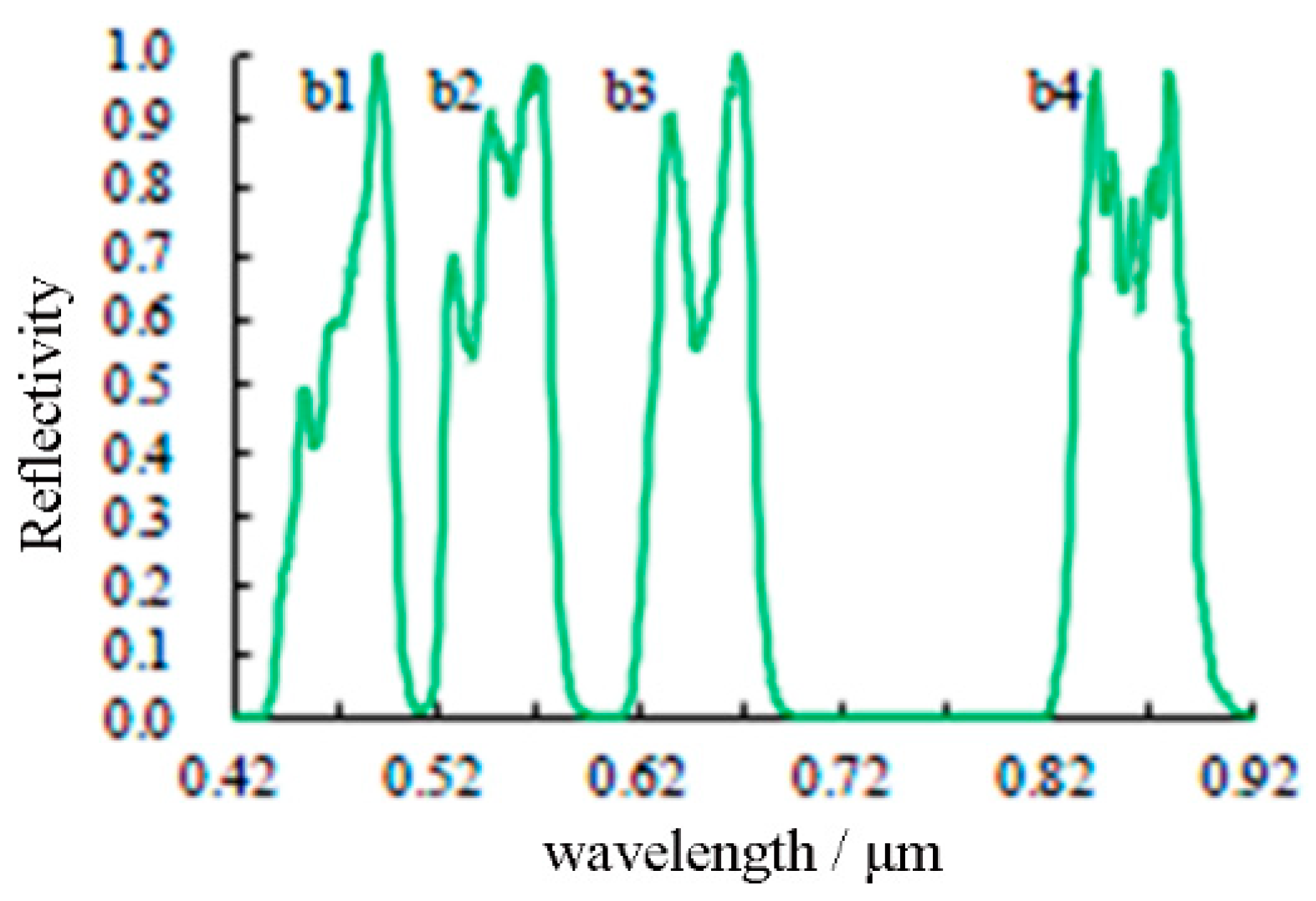
During the pre-processing of the data, various corrections and processing adjustments were made. These include geometric and radiometric correction, data exception processing, atmospheric correction, and cloud detection processing. The spectral response function of the FY-3C MERIS sensor used in data processing is shown in
Figure 2.
2.1.2. FPAR Products
In this paper, the FPAR products of MODIS, GEOV1, and GLASS were used for the cross-validation of FPAR inversion, and their specific characteristics are shown in
Table 2. The data preprocessing of FPAR products includes extracting sub-data sets, projections and transformations, splicing and cropping, and band operations (FPAR* scaling factors) to obtain a valid range of FPARs.
MODIS FPAR products: MOD15A2H products are available on the Level-1 and Atmosphere Archive & Distribution System Distributed Active Archive Center at Goddard Space Flight Center (LAADS DAAC) (
https://ladsweb.modaps.eosdis.nasa.gov/).
GEOV1 FPAR products: These products result in two outputs with a spatial resolution of 300 m and 1 km. The former was based on the PRoject for On-Board Autonomy–Vegetation (PROBA-V) sensor, with a time coverage from 2014 to the present. The latter was based on the SPOT Vegetation (SPOT-VGT) and PROBA-V sensor, with a time coverage from 1999 to the present. For this work, the former FPAR product with a better spatial resolution (300 m) was selected. Data for GEOV1 FPAR are available on the Copernicus Global Land Service (CGLS,
https://land.copernicus.eu/global/).
GLASS FPAR products: GLASS09A01 products were released by the Center for Global Change Data Processing and Analysis at Beijing Normal University. Data for the GLASS FPAR products were taken from the National Earth System Science Data Sharing Service Platform (
http://www.geodata.cn/thematicView/GLASS.html).
2.1.3. Supplementary Data
Land cover data: The MCD12Q1 data, which are obtained from the MODIS data by combining Terra and Aqua, have a spatial resolution of 500 m and provide five global land cover classification systems. These systems are the International Geosphere-Biosphere Programme (IGBP) classification system, the IGBP revision from the University of Maryland (UMDD) classification system, and other services for estimating LAI/FPAR, net primary productivity (NPP) and plant function type (PFT), respectively. The IGBP system has been selected and applied for data classification in this study.
Surface reflectance data (MOD09 data): This article used the MOD09GA product (based on Terra satellite product data), which has a spatial resolution of 500 m and provides a global daily ground-based basic reflectivity. These data are accessible from the LAADS DAAC (
https://ladsweb.modaps.eosdis.nasa.gov/).
The FPAR product of the Heihe research area [
25]: This product was provided by the Cold and Arid Regions Science Data Center at Lanzhou (
http://westdc.westgis.ac.cn). The data are based on the canopy Bidirectional Reflectance Distribution Function (BRDF) model and the LUT algorithm, with a spatial resolution of 1 km and a temporal resolution of 8 days.
2.2. Methods
2.2.1. Simulating FPAR Based on the PROSAIL Model
The PROSAIL model, which consists of the SAIL canopy bidirectional reflection model and the PROSPECT leaf optical property model, is a widely used model in vegetation parameter inversion [
26]. The PROSPECT model is a radiation-transfer model based on a plate model modified by Allen (1969) for simulating the directional hemispherical reflectance and transmissivity of various green monocots and dicots and senescent leaves, expressing leaf optical properties of 400–2500 nm. On the other hand, the SAIL model applies to the SUIT model to simulate the reflectivity of the leaf canopy’s direction under certain observational conditions by inputting the LAI, the leaf angle distribution, and other parameters [
27,
28].
As a secondary parameter of the PROSAIL model, FPAR needs to be converted into direct input parameters (such as LAI) or calculated between radiation transmissions. From the perspective of energy balance, the expression of FPAR is
Equation (1) can also be converted to:
where
is the visible albedo at the top of the canopy and
is the soil albedo,
, which is the transmittance of PAR emitted from the bottom of the canopy. This algorithm ignores
and results in the following FPAR expression (Equation (3)) [
28]:
The PAR incident on the surface canopy of the blade includes direct radiation and scattering, so the transmittance corresponding to the PAR incident on the soil portion is further expressed as
where
and
, respectively, refer to the transmittance of direct incident PAR and scattered incident PAR and
refers to the sky light scale factor. The transmittance of the canopy is related to various parameters, including sensor parameters and plant parameters. If the absorptivity of the leaves is
, the transmittance of the direct incident PAR can be approximated by the exponential model (Equation (5)) from Campbell and Norman (1998). If the scattered radiation comes from all directions, the transmittance of the scattered incident PAR can be obtained by integrating the transmittance of the direct incident PAR in each incident direction (Equation (6)) [
29].
where
is the clumping index (CI), angle
is the solar zenith angle, and
is the extinction coefficient of the canopy for PAR. The clumping index is determined by the spatial distribution pattern of the leaves, and the global clumping index of different vegetation types is shown in
Table 3 (for shrubs, broadleaf forests, and needleleaf forests).
Another algorithm for simulating FPAR is based on LAI (alternate algorithm). LAI is a direct input parameter in the PROSAIL model, which can be directly obtained from the model inversion. As the secondary parameter of the PROSAIL model, FPAR is retrieved by using the relationship of LAI/FPAR (Equation (7)), which is also used in the Monsi and Sacki models [
30]. This process ensures that LAI and FPAR maintain good consistency to some extent:
where K is the extinction coefficient. Among the appropriate factors, the LAI and the solar zenith angle have a certain influence on the extinction coefficient (K), which is mostly between 0.3 and 1.5 for the plant community under investigation; the value of K is about 0.3–0.5 for grasslands and mostly above 0.7 for herbs and shrubs [
30].
2.2.2. The Inversion of FPAR Based on the Look-Up Table
The LUT algorithm is simple, easy to operate, and has good precision. This algorithm is widely used in the radiation transfer model. In this paper, the canopy reflectance data obtained from the simulation of the model is compared with the reflectance of the pre-processed satellite data, and a look-up table for the reflectivity of different channels (blue, green, red, and near infrared) is established. Finally, the residual optimization parameter matrix (Equation (8)) was computed to obtain the simulated reflectance value with the smallest error, which was used to invert the model parameters:
where
R is the surface reflectance from the FY-3C date and
r is the canopy reflectance estimated from the PROSAIL model.
3. The Inversion Strategy of FPAR
The Heihe area was selected in this experiment, and, for this area, the FY-3C MERSI data and MODIS surface reflectance data (MOD09GA) were used to extract the required data. In order to obtain two inverted FPAR products, namely FY-FPAR and MOD09-FPAR, from two different satellites sources, the same PROSAIL model and the LUT algorithm were applied.
3.1. Applicability Analysis
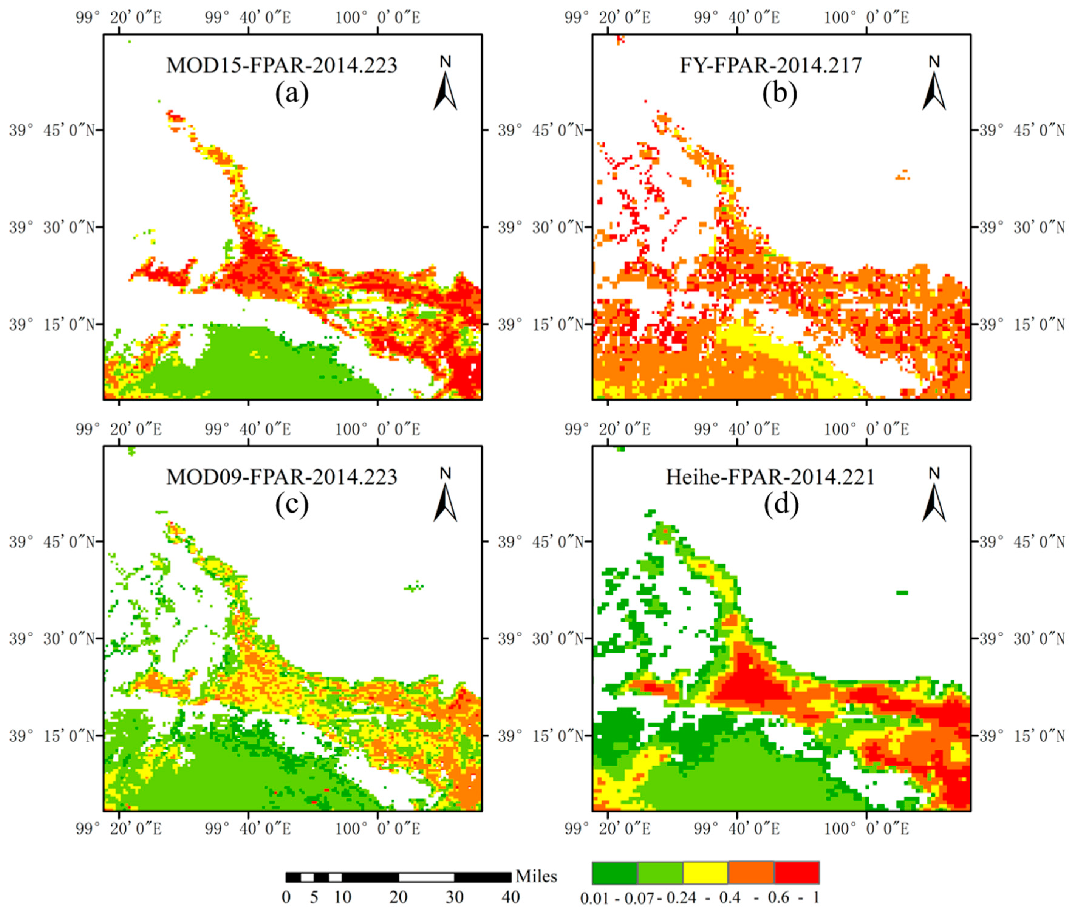
A comparison of the FPAR inversion results and FPAR products in the Heihe research area was conducted to determine the effects of the differences in remote sensing data sources, applied models, and algorithms. This comparison also helps to prove the validity of the method and adjust the inversion strategy according to the characteristics of the FY-3C data. The two inverted FPAR results, MOD09-FPAR and FY-FPAR (which were obtained from MOD09GA and FY-3C MERSI, respectively, by using the same PROSAIL model and LUT algorithm), and the MODIS FPAR product (referred to as MOD15-FPAR) were compared against each other relative to the Heihe FPAR product (known as HeiHe-FPAR), published by the Cold and Arid Region Science Data Center (
Figure 3).
As shown in
Figure 3a,b, based on the same PROSAIL model and LUT algorithm, the difference in remote sensing data leads to inconsistent results. The FPAR from the FY-3C data was clearly high, especially in low-value areas. As shown in
Figure 3a,c, based on the same MOD09 data, different algorithms lead to different results. Based on the correlation analysis, the FPAR results of
Figure 3a–c correlated with the Heihe-FPAR of
Figure 3d, and the scatter plots are shown in
Figure 4.
As shown in
Figure 4a,c, based on the same MOD09 data, the correlation between MOD09-FPAR and Heihe-FPAR was higher than that of MOD15-FPAR and Heihe-FPAR (0.8922 > 0.7991). This shows that the applied method (PROSAIL model and LUT algorithm) is feasible.
On the other hand, the degree of agreement between MOD09-FPAR and Heihe-FPAR (R = 0.8922) is significantly greater than that between FY-FPAR and Heihe-FPAR (R = 0.5746), as shown in
Figure 4a,b. In other words, the correlation between FY-FPAR and Heihe-FPAR is relatively low because the difference in the band range between the FY-3C MERSI data and the MOD09GA data (which is not a complete coincident), and the correlation of the reflectance of the different channels with blue, green, red, and near infrared, is about 0.6 (as shown in
Table 4).
Therefore, since the feasibility of the applied model and algorithm has already been proven, the inversion of FPAR from FY-3C data needs to be combined with the characteristics of the Fengyun satellite to optimize the inversion strategy.
3.2. The Strategy of Inversion
3.2.1. Spectral Convolution
The PROSAIL model was the first model used in the inversion of FPAR from FY-3C MERSI data. The simulated reflectivity was then convoluted in order to meet the characteristics of the FY-3C data. Thus, the final reflectance data was obtained by convolving the simulated spectral curve with the MERSI sensor’s spectral response function (as shown in
Figure 2) with the blue, green, red, and near infrared bands using the reference formula [
31]:
where
is the reflectivity on the specified band
, which is obtained by convolving the simulated spectral curve through the sensor spectral response function;
;
refers to the simulated reflectivity;
is the spectral response function corresponding to the i-th channel; and
refers to the outer layer of the atmosphere, known as the Solar irradiance (solar constant). The solar constant is the 1366.1 Wm-2 [
32].
3.2.2. Vegetation Division
The PROSAIL model involves many parameters that require sensitivity analysis to set a reasonable range. The study finds that the reflectance spectrum of sparse vegetation is mainly affected by soil reflectivity, while the reflectance spectrum of dense vegetation is mainly affected by the biochemical composition of vegetation. Therefore, we classified the study region into two classes for the inversion of FPAR based on the value of the normalized difference vegetation index (NDVI) (
Table 5).
For the partitioning indicator NDVI of the vegetation partition, the effective value was [−1,1]. When NDVI ≤ 0, there was no vegetation in the area; then, we had a sparse and lush subdivision in the interval of NDVI in [0,1]. The threshold set in this paper was 0.4, based on our prior knowledge of the relevant references and experimental statistics we have conducted. Hence, the application of the partition operation for different land types depended on the actual prevailing situation.
3.2.3. Parameterization of Different Vegetation Types
The parameters of different vegetation types are quite different: The closer to the parameter range of the PROSAIL model setting to the true value, the higher the inversion precision will be. Consequently, the different parameter range settings of different vegetation types will be different according to the features of those vegetation types. In this paper, we considered five typical vegetation types: grassland, cropland, shrub, broadleaf forest, and needleleaf forest. Relevant studies have shown that the distribution of broadleaf forests and needleleaf forests is different from that of other types and has higher LAI values (4.0 to 6.0), while for other vegetation types, the LAI value is usually less than 2.0. In this work, typical research areas for grassland, cropland, shrub, broadleaf forest, and needleleaf forest were selected: the Hulunber, Yucheng, Shapotou, Dinghushan, and Changbai Mountains in China (
Figure 1).
Therefore, combined with the vegetation division and prior knowledge of previous studies, the PROSAIL model parameter settings for different vegetation types are shown in
Table 6. The left and right boundaries and the step sizes of the parameters had two parts—sparse areas and dense areas—and were divided by “/”. Among these parameters, tts, tto, and psi were obtained from the angle information of FY-3C MERSI (the value of the angle data was the average value of each pixel in the study area), and other parameters were set according to prior knowledge and constant adjustment to obtain reasonable values or ranges.
4. Results and Analysis
In this article, one image with less cloud and better quality in each month has been selected to perform batch inversion of the long-term FPAR from the 2014 annual FY-3C MERSI data. Based on the parameterization of the PROSAIL model (
Table 6), the parameter ranges of grassland, cropland, shrub, broadleaf forest, and needleleaf forest have been taken as the inputs into the PROSAIL model to simulate FPAR, and a look-up table has been constructed to invert FPAR. The inversion results are referred to as FYgrass-FPAR\FYcropland-FPAR\FYshrub-FPAR\FYbroadleaf-FPAR\FYneedleleaf-FPAR for different vegetation types, and the date of the image is roughly regarded as the FPAR value of the current month. Finally, the MODIS/GEOV1/GLASS FPAR products were selected to analyze the accuracy of the FPAR inversion results using cross-validation.
4.1. The Inversion Results of FPAR
The annual FY-FPARs for the five research areas of grassland, cropland, shrub, broadleaf forest, and needleleaf forest were inverted successfully based on the inversion strategy from the FY-3C data.
The seasonal variation of FYgrass-FPAR in the HulunBer grassland study area was distinct (
Figure 5a). The FPAR values for the whole year showed a general trend of rising first and then decreasing. In addition, there was a large degree of spatial loss in January–February and November–December. This loss was due to the low temperatures in these months, and the inversion of FPAR was affected by snow or other atmospheric factors.
The seasonal variation of FYcropland-FPAR in the Shangqiu cropland study area was clearer (
Figure 5b). The high value period of FPAR was in July and August, located in the west of the Shangqiu Research Area, while the low value period of FPAR was in February, June, and October. This annual distribution seemed to indicate a resurgence that met the growth curve of the two seasonal crops.
The seasonal variation of FYshrub-FPAR in the Shapotou shrub study area was noticeable (
Figure 5c), and the annual FPAR was generally low. In this area, the high value period of FPAR ran from June to September, the vegetation coverage was high, and the FPAR values were lower at other times, most of which were lower than 0.2 (and lower than 0.1 in January and February). The seasonal variation of the shrub FPAR was consistent with the law of vegetation growth, but this shrub had the characteristics of shrub vegetation itself, and there was a difference in the distribution of FPAR.
The seasonal variation of FYbroadleaf-FPAR in the Dinghushan broadleaf forest study area was unclear (
Figure 5d). Its overall FPAR was higher than 0.6 in 2014. In this area, the FPAR was higher from September to December, with most FPAR values greater than 0.8. This was because the Dinghushan broadleaf forest study area belonged to a deciduous broadleaf forest; moreover, defoliation occurred in autumn and winter after September, thereby covering the exposed land and increasing the FPAR value.
The seasonal variation of FYneedleleaf-FPAR in the Changbai Mountain needleleaf forest study area was relatively obvious (
Figure 5e). The FPAR values for 2014 showed a trend of first increasing and then declining. The FPARs of June–August were higher; most of them were greater than 0.7. However, the FPAR of October–December and January–March were relatively low (similar to the grassland), in line with the seasonal growth of vegetation.
4.2. Cross-Validation
The cross-validation of this paper selected the FPAR products of MODIS, GEOV1, and GLASS (referred to as MODIS-FPAR, GEOV1-FPAR, and GLASS-FPAR), as well as FY-FPAR, to verify the accuracy of the same spatial range at the same time and to analyze the spatial consistency, time consistency, and relevance.
4.2.1. Spatial Consistency
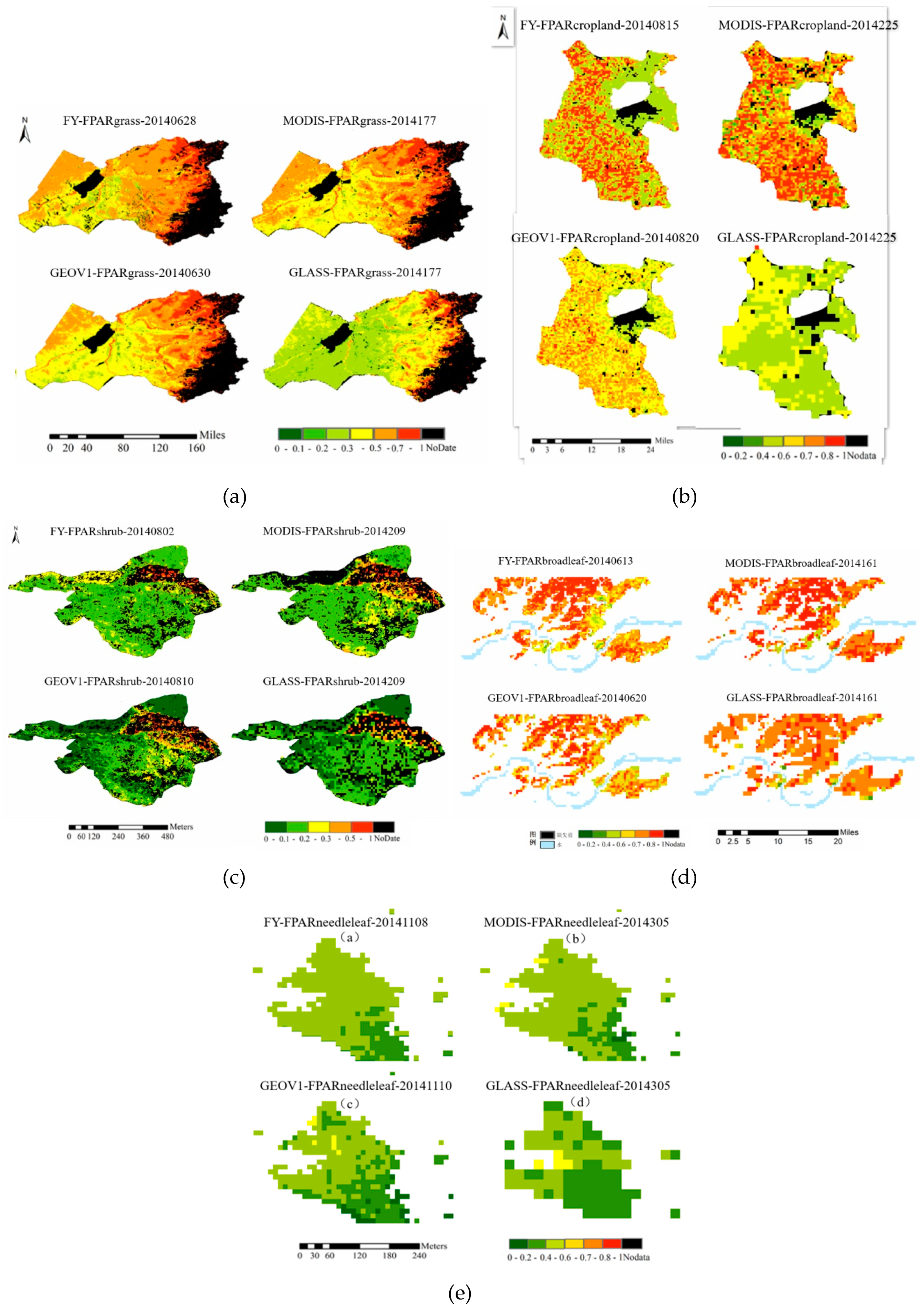
Spatial consistency was verified by comparing the spatial distribution of FY-FPAR with that of MODIS-FPAR, GEOV1-FPAR, and GLASS-FPAR. A FY-FPAR was randomly selected to display the spatial distribution comparison map (
Figure 5). The results show that FY-FPAR maintained a good spatial consistency with MODIS-FPAR, GEOV1-FPAR, and GLASS-FPAR.
The difference frequency was used to analyze the differences between FY-FPAR and MODIS-FPAR and GEOV1-FPAR, and GLASS-FPAR. Using the FY-FPAR data as the statistical data source, we calculated the difference between the FY-FPAR and the three FPAR products for the MODIS-FPAR, GEOV1-FPAR, and GLASS-FPAR in the study area. The difference results were calculated to obtain the frequency distribution. The difference frequency of the grassland, cropland, shrub, broadleaf forest, and needleleaf forest is shown in
Figure 6.
Figure 6 exhibits that the difference frequencies of the grassland, cropland, shrub, broadleaf forest, and needleleaf forest between FY-FPAR, MODIS-FPAR, and GEOV1-FPAR. GLASS-FPAR was concentrated around 0 (in the ±0.4 interval), which is a reasonable range. The peak of the difference frequency was almost at 0, and the spatial consistency was relatively good.
4.2.2. Temporal Consistency
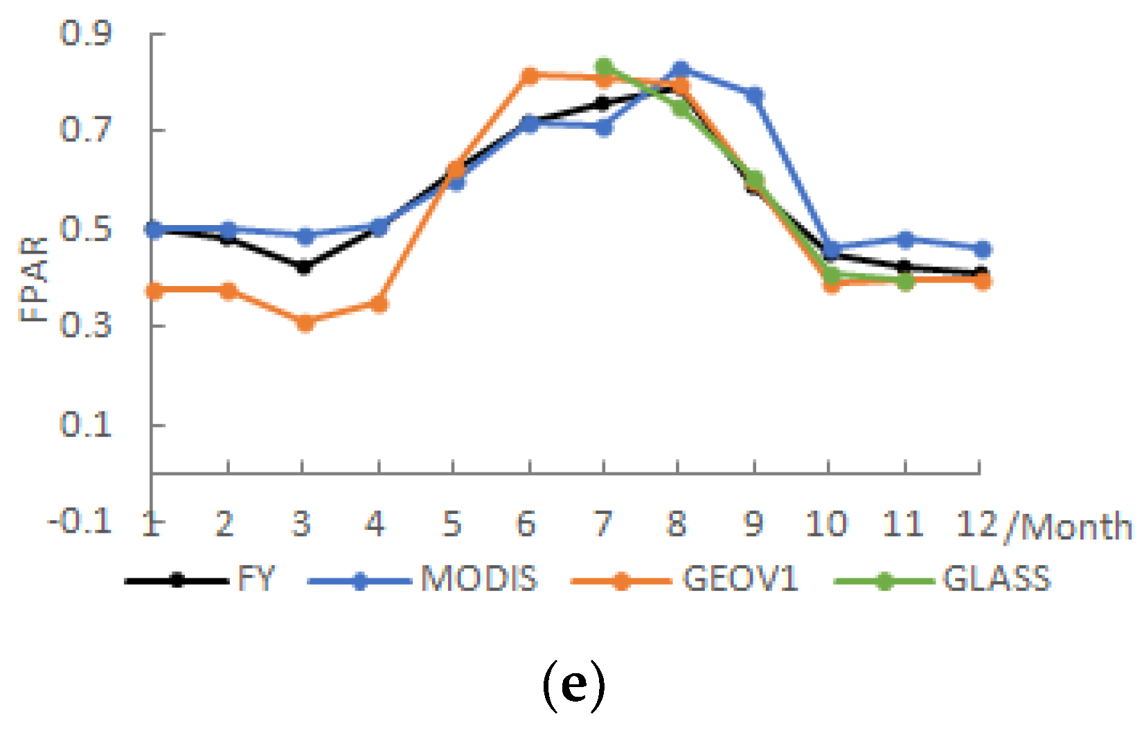
Compared to the time series data of the FY-FPAR, MODIS-FPAR, GEOV1-FPAR, and GLASS-FPAR of various vegetation types in 2014 (
Figure 7), FY-FPAR and the other three products all showed good consistency over their time series.
Overall, the annual FY-FPAR of the grassland, cropland, shrub, broadleaf forest, and needleleaf forest maintained a high consistency with the corresponding MODIS-FPAR, GEOV1-FPAR, and GLASS-FPAR in the time-series (GLASS-FPAR only included the data from June to November). The FPAR time-series curves of the five vegetation types remained smooth and continuous. Among these curves, the FY-FPARs of the grassland, shrub, and needleleaf forest, with the other three FPAR products, showed a general increase in their trends at the beginning, which dropped off after reaching its maximum around July and August. This change can be clearly explained in terms of the seasonal growth regulation of vegetation, which was consistent with the characteristics of a higher FY-FPAR in summer and a lower FY-FPAR in winter. The change of the broadleaf forest FY-FPAR alongside the other three FPAR products in the time-series was not clear and remained relatively stable. The FY-FPAR of the cropland was more special in the time-series, showing a trend of increasing first and then falling, before going up and then falling, including two peaks in April and July and three troughs in February, June, and October, which are associated with the seasonal growth regulation of double seasonal crops and highlight the information on crop rotation. In addition, the FPAR time-series curve of the shrub area was significantly different from that of other vegetation types, and its FY-FPAR was generally higher than its GEOV1-FPAR and GLASS-FPAR, which were closer to the MODIS-FPAR. It was inferred that the pixels of the reflectance data before inversion contained mixed pixels of shrubs and croplands and shrubs and grasses, which gave the FY-FPAR a certain degree of variation.
4.2.3. Correlation Analysis
In this paper, the correlation coefficient (R) and root mean square error (RMSE) were used as the correlation indicators between FY-FPAR and other FPAR products. The normal range of the correlation coefficient (R) is from 0 to 1. The closer it was to 1, the greater the correlation between the two sets of data. The RMSE is widely used as a way to measure the deviation between two sets of data. The closer the RMSE is to 0, the better the relationships between the data. The correlation statistics of FY-FPAR and MODIS-FPAR, GEOV1-FPAR, and GLASS-FPAR are exhibited in
Table 7.
Overall, the annual FY-FPAR of the grassland, cropland, shrub, broadleaf forest, and needleleaf forest areas had a high correlation with that of the other three FPAR products in 2014, and higher correlations were concentrated in the period when vegetation was lusher. Especially for grassland and cropland, the correlation coefficient (R) of the FY-FPAR and FPAR products in the lush period of the grassland (June–October) was as follows: with MODIS-FPAR: R = 0.5549/RMSE = 0.1103; with GEOV1-FPAR: R = 0.6102/RMSE = 0.1157; with GLASS-FPAR: R = 0.5827/RMSE = 0.1205. The correlation coefficient (R) of the FY-FPAR and FPAR products in the lush period of cropland (January, February, April, July, and November) was as follows: with MODIS-FPAR: R = 0.6012/RMSE = 0.1151; with GEOV1-FPAR: R = 0.5913/RMSE = 0.131; with GLASS-FPAR: R = 0.495/RMSE = 0.1377. This was much higher than the annual correlation coefficient (R) of the respective vegetation type. This occurred because the vegetation in the sparse period of vegetation had more exposed land, and the reflection spectrum of the vegetation was mainly affected by the soil’s reflectivity, which affected the inversion accuracy.
The correlation coefficient (R) of FY-FPAR and MODIS-FPAR was as follows: cropland (lush period) > cropland (Annual) > grassland (lush period) > needleleaf forest > broadleaf forest > grassland (Annual) > shrub. The correlation coefficient (R) of FY-FPAR and GEOV1-FPAR was grassland (lush period) > cropland (lush period) > grassland > needleleaf forest > shrub > broadleaf forest. The correlation coefficient (R) of FY-FPAR and GLASS-FPAR was grassland > needleleaf forest > cropland > broadleaf forest > shrub.
In summary, the inversion accuracy of FY-FPAR for cropland and grassland areas during the lush vegetation period was relatively high; the inversion accuracy was good for broadleaf forest and needleleaf forest, and the inversion accuracy for shrubs was relatively low, as shown in
Table 7. Thus, the annual FPAR of the shrubs was low, indicating that the inversion strategy based on FY-3C data was more suitable for the inversion of the FPAR of high-value areas. In addition, due to the difference in the surface reflectance data used by FY-FPAR and other FPAR products during inversion (as shown in
Table 4), the FY-FPAR was relatively suitable for cropland and grassland during the lush period and in the broadleaf forest and needleleaf forest. The inversion of shrub FPAR also needed to consider the factors affecting bare soil.
4.3. Error Analysis
The inversions of the FPARs from the FY-3C data and the MODIS, GEOV1, GLASS FPAR products had good consistency in time and space, but there remained a certain range of errors. The reasons for these errors are summarized as follows:
The difference in surface reflectance. The inversion directly used the top-of-reflectance from the FY-3C MERSI data. The MODIS-FPAR products were based on MOD09 surface reflectance products. The GEOV1-FPAR products were based on spot/vegetation surface reflectance products. In addition, the spectral ranges of their red, green, blue, and near red bands were not the same, and their reflectivity was also inconsistent, suggesting that the difference in reflectance data affected the inversion results of FPAR.
Spatial misalignment. Each product had geometric accuracy and pixel location errors, where the geographic location of the FY-3C MERSI data had a non-uniform geometric error of 2–10 pixels (causing a mismatch), which could also contribute to the inconsistency among the data.
FY-3C image pre-processing was not perfect. De-clouding during data pre-processing was not very good for thin cloud removal and cloud-snow differentiation. Cloud-snow reflectance data brought into the model could cause large errors.
Limitations of the physical model. Each product had a different model and different algorithms. Although there was strict physical theory support, these differences may have caused errors for the same area.
5. Discussion
The initial objective of the study was to obtain an accurate FPAR using remote sensing data. We considered two strategies for obtaining FPAR parameters using remote sensing. One strategy was based on the empirical statistical model, which is simple in calculation and has few parameters, but remains highly dependent on geographical location, topography, and vegetation type. The other strategy was to use a physical model. This model is more feasible than the first model when considering the energy balance in radiation transmission, although it has more variables; thus, this latter model was adopted for this study. The inversion of FPAR using domestic satellites combined with physical models is rare, and no long-term or large-scale serial FPAR products have been formed based on Chinese satellite data. Unlike the HJ-1 data used by Chen, Ma, and Li et al., this study uses FY-3C MERSI data and experiments on five different vegetation types in different terrains in China that are more representative [
21,
22,
45]. This research had certain reference values for the promotion and application of Chinese satellites and the generation of Chinese satellite FPAR products. Based on the FY-3C MERSI data, this study introduced the PROSAIL model and LUT algorithm and proposed an FPAR inversion strategy. The cross-validation confirmed that the proposed method had high accuracy, but there were still limitations in the study, which offer some directions for future research.
In this study, the classification of vegetation types during the early stages of FPAR inversion was based on MODIS land cover products (MCD12Q1). The time resolution of MCD12Q1 was 1 year, and its spatial resolution was 500 m. There were classification errors for the seasonal variation of FPARs for different vegetation types; these errors produced mixed pixels in the inversion accuracy, which made the inversion results lack objectivity. Later studies could extract time-series land cover classification data from FY-3C MERSI data, so the classification data could also have seasonal variation characteristics.
Due to a ubiquitous ill-posed problem, the inversion of quantitative remote sensing always uses a small number of parameters to infer complicated ground parameters, which are known to be much less than unknown. This study used prior knowledge to alleviate this ill-posed problem as much as possible, but our prior knowledge was limited and there were still many uncertainties in the inversion of FPAR. For model parameter settings of different vegetation types, relying on prior knowledge is feasible, but it is more precise to base such settings on actual measurements. In addition, it was reasonable to use NDVI to divide vegetation into different densities, but the threshold setting needs to be further explored according to different vegetation types.
In the cross-validation of FY-FPAR and MODIS-FPAR, GEOV1-FPAR, and GLASS-FPAR, the spatial consistency, time consistency, and correlation analyses were applied to objectively evaluate the inversion accuracy of FY-FPAR and also the error analysis (
Section 4.3). However, using only the data of 2014, which were limited in time and frequency to account for seasonal variations, may have caused limitations in quantitative analysis. Subsequent studies can consider adding FY-3C MERSI data for many years to compare the seasonal variation between FY-FPAR and other FPAR products. Thus, a comparison of monthly FPARs, using the multi-year average of the month, will reduce the noise of the time-series curve. In addition, for human and material conditions, it is possible to more accurately evaluate the inversion accuracy by considering a comparison of the measured data of the FPAR.
Lastly, the inversion of FPAR in this paper was based on the inversion of FPAR for five types of vegetation: grassland, cropland, shrub, broadleaf forest, and needleleaf forest. To form FPAR products, different vegetation types needed to be spliced and fused. An overall analysis and evaluation was then conducted to prepare time-series FPAR products from FY-3C data.
6. Conclusions
In this paper, an inversion strategy of FPAR for FY-3C MERSI data was proposed and applied to five types vegetation, including grassland, cropland, shrub, broadleaf forest, and needleleaf forest, from various parts of the country. The FPAR product data of MODIS, GEOV1, and GLASS were selected for cross-validation and correlation analyses.
The results were as follows:
The FY-FPAR of the five different vegetation types in the grassland, cropland, shrub, broadleaf forest, and needleleaf forest indicated a good correlation with MODIS-FPAR, GEOV1-FPAR, and GLAS-FPA.
In terms of spatial distribution, the difference frequency between FY-FPAR and the other three FPAR products was concentrated around 0 (+0.4 interval), which is an acceptable dynamic range. The time-series curve was close to the FPAR products and maintained good consistency.
FY-FPAR was relatively more suitable for the inversion of grasslands and croplands during the lush period than to broadleaf forests and needleleaf forests, whereas, the inversion of shrub FPAR had to consider the influence of the underlying surface.
The inversion strategy of FPAR based on the PROSAIL model provided a basis for generating large-scale and long-range FPAR products for the FY-3C MERSI data.
Author Contributions
W.H. and W.X. proposed the original idea for the study; J.S. and X.L. performed the experiments and processed and analyzed the data, J.S., X.L., and W.X. wrote the original manuscript. W.H., J.S., and W.X. reviewed the paper. All authors have read and agreed to the published version of the manuscript.
Funding
This research was funded by the Sichuan Key and Research Program (No. 2018GZDZX0034), Sichuan Science and Technology Program (No.2018GZDZX0014), Sichuan Science and Technology Program (No. 2019YFG0202), Key Laboratory of Equipment Pre-research (No. 6142A010301) and Hebei Key and Research Program (No. 19255901D).
Acknowledgments
We would like to thank the journal’s editors and reviewers for their kind comments and valuable suggestions to improve the quality of this paper.
Conflicts of Interest
The authors declare no conflict of interest.
References
- Huang, J.; Gómez-Dans, J.; Huang, H.; Ma, H.; Wu, Q.; Lewis, P.; Liang, S.; Chen, Z.; Xue, J.; Wu, Y.; et al. Assimilation of remote sensing into crop growth models: Current status and perspectives. Agric. Meteorol 2019, 276–277, 107609. [Google Scholar] [CrossRef]
- Yang, N.; Liu, D.; Feng, Q.; Quan, X.; Zhang, L.; Ren, T.; Zhao, Y.; Zhu, D.; Huang, J. Large-Scale Crop Mapping Based on Machine Learning and Parallel Computation with Grid. Remote Sens. 2019, 11, 1500. [Google Scholar] [CrossRef] [Green Version]
- Zhuo, W.; Huang, J.; Li, L.; Zhang, X.; Ma, H.; Gao, X.; Huang, H.; Xu, B.; Xiao, X. Assimilating Soil Moisture Retrieved from Sentinel-1 and Sentinel-2 Data into WOFOST Model to Improve Winter Wheat Yield Estimation. Remote Sens. 2019, 11, 1618. [Google Scholar] [CrossRef] [Green Version]
- Huang, J.; Sedano, F.; Huang, Y.; Ma, H.; Li, X.; Liang, S.; Tian, L.; Zhang, X.; Fan, J.; Wu, W. Assimilating a synthetic Kalman filter leaf area index series into the WOFOST model to improve regional winter wheat yield estimation. Agric. Meteorol. 2016, 216, 188–202. [Google Scholar] [CrossRef]
- Huang, J.; Zhuo, W.; Li, Y.; Huang, R.; Sedano, F.; Su, W.; Dong, J.; Tian, L.; Huang, Y.; Zhu, D.; et al. Comparison of Three Remotely Sensed Drought Indices for Assessing the Impact of Drought on Winter Wheat Yield. Int. J. Digit. Earth 2018. [Google Scholar] [CrossRef]
- Huang, R.; Huang, J.; Zhang, C.; Ma, H.; Zhuo, W.; Chen, Y.; Zhu, D.; Wu, Q.; Lamin, R.M. Soil temperature estimation at different depths, using remotely sensed data. J. Integr. Agric. 2020, 19, 277–290. [Google Scholar]
- Ma, G.; Huang, J.; Wu, W.; Fan, J.; Zou, J.; Wu, S. Assimilation of MODIS-LAI into WOFOST model for forecasting regional winter wheat yield. Math. Comp. Modell. 2013, 58, 634–643. [Google Scholar] [CrossRef]
- Martinez, B.; Garcia-Haro, J.F.; Gilabert, A.M.; Camacho, F. Intercomparison and quality assessment of MERIS, MODIS and SEVIRI FAPAR; products over the Iberian Peninsula. Int. J. Appl. Earth Obs. Geoinf. 2013, 21, 463–476. [Google Scholar] [CrossRef]
- Mccallum, I.; Wagner, W.; Schmullius, C.; Shvidenko, A.; Obersteiner, M.; Fritz, F.; Nilsson, S. Comparison of four global FAPAR datasets over Northern Eurasia for the year 2000. Remote Sens. Environ. 2010, 114, 941–949. [Google Scholar] [CrossRef]
- Huang, J.; Tian, L.; Liang, S.; Ma, H.; Becker-Reshef, I.; Huang, Y.; Su, W.; Zhang, X.; Zhu, D.; Wu, W. Improving winter wheat yield estimation by assimilation of the leaf area index from Landsat TM and MODIS data into the WOFOST model. Agric. Meteorol. 2015, 204, 106–121. [Google Scholar] [CrossRef] [Green Version]
- Huang, J.; Ma, H.; Su, W.; Zhang, X.; Huang, Y.; Fan, J.; Wu, W. Jointly assimilating MODIS LAI and ET products into the SWAP model for winter wheat yield estimation. IEEE J. Sel. Top. Appl. Earth Obs. Remote Sens. 2015, 8, 4060–4071. [Google Scholar] [CrossRef]
- Myneni, R.B.; Ramakrishna, R.; Nemani, R.; Running, S.W. Estimation of global leaf area index and absorbed par using radiative transfer models. IEEE Trans. Geosci. Remote Sens. 2002, 35, 1380–1393. [Google Scholar] [CrossRef] [Green Version]
- Tian, Y.; Yu, Z.; Knyazikhin, Y.; Myneni, R.B. Prototyping of MODIS LAI and FPAR algorithm with LASUR and LANDSAT data. Geosci. Remote Sens. IEEE Trans. 2000, 38, 2387–2401. [Google Scholar] [CrossRef] [Green Version]
- Myneni, R.B.; Hoffman, S.; Knyazikhin, Y.; Privette, J.L.; Glassy, J.; Tian, Y.; Wang, Y.; Song, X.; Zhang, Y.; Smith, G.R. Global products of vegetation leaf area and fraction absorbed PAR from year one of MODIS data. Remote Sens. Environ. 2002, 83, 214–231. [Google Scholar] [CrossRef] [Green Version]
- Baret, F.; Weiss, M.; Lacaze, R.; Camacho, F.; Makhmara, H.; Pacholcyzk, P.; Smets, B. GEOV1: LAI and FAPAR essential climate variables and FCOVER global time series capitalizing over existing products. Part1: Principles of development and production. Remote Sens. Environ. 2013, 137, 299–309. [Google Scholar] [CrossRef]
- Nadine, G.; Bernard, P.; Michel, V.; Yves, G. The MERIS Global Vegetation Index (MGVI): Description and preliminary application. Int. J. Remote Sens. 1999, 20, 1917–1927. [Google Scholar]
- Baret, F.; Olivier, H.; Bernhard, G.; Patrice, B.; Bastien, M.; Mireille, H.; Béatrice, B.; Fernando, N.; Marie, W.; Olivier, S. LAI, fAPAR and fCover CYCLOPES global products derived from VEGETATION: Part 1: Principles of the algorithm. Remote Sens. Environ. 2007, 110, 275–286. [Google Scholar] [CrossRef] [Green Version]
- Coca, F.C.D.; Garcia-Haro, J.; Melia, J. Prototyping algorithm for retrieving FAPAR using MSG data in the context of the LSA SAF project. In IEEE International Geoscience and Remote Sensing Symposium, Barcelona; IEEE: Piscataway, NJ, USA, 2007; pp. 1016–1020. [Google Scholar]
- Zhu, Z.; Bi, J.; Pan, Y. Global Data Sets of Vegetation Leaf Area Index (LAI) 3g and Fraction of Photosynthetically Active Radiation (FPAR) 3g Derived from Global Inventory Modeling and Mapping Studies (GIMMS) Normalized Difference Vegetation Index (NDVI3g) for the Period 1981 to 20. Remote Sens. 2013, 5, 927–948. [Google Scholar]
- Xiao, Z.; Shunlin, L.; Rui, S.; Jindi, W.B.J. Estimating the fraction of absorbed photosynthetically active radiation from the MODIS data based GLASS leaf area index product. Remote Sens. Environ. 2015, 171, 105–117. [Google Scholar] [CrossRef]
- Chen, X.; Jihua, M.; Bingfang, W.; Jianjun, Z.; Du, X.; Feifei, Z.; Liming, N. Monitoring corn FPAR based on HJ-1 CCD. Trans. Chin. Soc. Agric. Eng. 2010, 26 (Suppl. 1), 241–245. [Google Scholar]
- Xiaoyu, L.; Fei, L.; Yuhai, B.; Zhenwang, L.; Baohui, Z.; Ruirui, Y.; Xiaoping, X. Validation and Analysis of MODIS/FPAR Product based on HJ-1CCD Image in Hulunber Grassland. Remote Sens. Technol. Appl. 2015, 30, 1129–1137. [Google Scholar]
- Yang, J. Development and Applications of China’s Fengyun (FY) Meteorological Satellite. Spacecr. Eng. 2008, 17, 23–27. [Google Scholar]
- Xiuqing, H.; Xu, A.N.; Ronghua, W.A.; Chen, L. Performance assessment of FY-3C/MERSI on early orbit. In Proceedings of the SPIE, Beijing, China, 13–17 October 2014. [Google Scholar] [CrossRef]
- Yuan, L.; Wenjie, F.; Xiru, X.; Gaoxing, C. A new FAPAR retrieval model for continuous vegetation. In Proceedings of the 2013 IEEE International Geoscience and Remote Sensing Symposium, Melbourne, Australia, 21–26 July 2013; IEEE: Piscataway, NJ, USA, 2013; pp. 3052–3055. [Google Scholar]
- Jacquemoud, S.; Wout, V.; Frédéric, B.; Cédric, B.; Zarco-Tejada, P.J.; Gregory, P.A.; Christophe, F.; Susan, L.U. PROSPECT+SAIL models: A review of use for vegetation characterization. Remote Sens. Environ. 2009, 113, S56–S66. [Google Scholar] [CrossRef]
- Badhwar, G.D.; Verhoef, W.; Bunnik, N.J.J. Comparative study of suits and sail canopy reflectance models. Remote Sens. Environ. 1985, 17, 179–195. [Google Scholar] [CrossRef]
- Huang, J.; Ma, H.; Sedano, F.; Lewis, P.; Liang, S.; Wu, Q.; Su, W.; Zhang, X.; Zhu, D. Evaluation of regional estimates of winter wheat yield by assimilating three remotely sensed reflectance datasets into the coupled WOFOST–PROSAIL model. Eur. J. Agron. 2019, 102, 1–13. [Google Scholar] [CrossRef]
- Shunlin, L.; Jie, Z.; lijun, C.; Xiang, Z.; Jun, Y. Production and Application of Remote Sensing Products for Global Change; Science Press: Beijing, China, 2017; pp. 255–260. [Google Scholar]
- Ruimy, A.; Saugier, B.; Dedieu, G. Methodology for the estimation of terrestrial net primary production from remotely sensed data. J. Geophys. Res. Atmos. 1994, 99, 5263–5283. [Google Scholar] [CrossRef]
- Rong-Hua, W.; Jun, Y.; Zhong, D.; Jingjing, L. Impacts of Spectral Response Differences on SNO Calibration-study Examples of FY-3A/MERSI and EOS/MODIS. Remote Sens. Inf. 2011, 2, 51–57. [Google Scholar]
- Gueymard, C.A. The sun’s total and spectral irradiance for solar energy applications and solar radiation models. Sol. Energy 2004, 76, 423–453. [Google Scholar] [CrossRef]
- Gang, L.; Zhang, H.; Daolong, W.; Hongbin, Z.; Xiaoping, X. Remote Sensing Inversion Approach for FPAR of Temperate Meadow Grassland based on PROSAIL Model. Chin. J. Grassl. 2014, 36, 61–69. [Google Scholar]
- Dasong, X. Object-Oriented Inversion Method and Application of Grassland Vegetation Variables. Master’s Thesis, University of Electronic Science and Technology of China, Chengdu, China, 2017. [Google Scholar]
- Li, G.; Hua, Z.; Wenjie, F.; Hongbin, Z.; Xiaoping, X. Validation of MODIS FAPAR in the Hulunber grassland of China. Trans. Chin. Soc. Agric. Eng. 2010, 26, 217–224. [Google Scholar]
- Li, H.; Gaohuan, L.; Qingsheng, L.; Zhongxin, C.; Chong, H. Retrieval of winter wheat leaf area index from Chinese GF-1 satellite data using the PROSAIL model. Sensors 2018, 18, 1120. [Google Scholar] [CrossRef] [PubMed] [Green Version]
- Hongliang, F.; Wenjuan, L.; Shanshan, W.; Chongya, J. Seasonal variation of leaf area index (LAI) over paddy rice fields in NE China: Intercomparison of destructive sampling, LAI-2200, digital hemispherical photography (DHP), and AccuPAR methods. Agric. For. Meteorol. 2014, 198–199, 126–141. [Google Scholar] [CrossRef]
- Chen, W.; Cao, C.; He, Q.; Guo, H. Quantitative estimation of the shrub canopy LAI from atmosphere-corrected HJ-1 CCD data in Mu Us Sandland. Sci. China 2010, 53, 26–33. [Google Scholar] [CrossRef] [Green Version]
- Li, X.; Fangjie, M.; Huaqiang, D.; Guomo, Z.; Xiaojun, X.; Han, N.; Shaobo, S.; Guolong, G.; Chen, L. Assimilating leaf area index of three typical types of subtropical forest in China from MODIS time series data based on the integrated ensemble Kalman filter and PROSAIL model. ISPRS J. Photogramm. Remote Sens. 2017, 126, 68–78. [Google Scholar] [CrossRef]
- Maire, G.L.; Christophe, F.; Kamel, S.; Daniel, B.; Jean, Y.P.; Nathalie, B.; Hélène, G.; Hendrik, D.; Eric, D. Calibration and validation of hyperspectral indices for the estimation of broadleaved forest leaf chlorophyll content, leaf mass per area, leaf area index and leaf canopy biomass. Remote Sens. Environ. 2008, 112, 3846–3864. [Google Scholar]
- Shabanov, N.V.; Wang, Y.; Buermann, W.; Dong, J.; Hoffman, S.; Smith, G.R.; Tian, Y.; Knyazikhin, Y.; Myneni, R.B. Effect of foliage spatial heterogeneity in the MODIS LAI and FPAR algorithm over broadleaf forests. Remote Sens. Environ. 2003, 85, 410–423. [Google Scholar] [CrossRef] [Green Version]
- Liu, T.; Zhao, X.; Haihua, S.; Hui-Feng, H.; Wenjiang, H.; Jingyun, F. Spectral feature differences between shrub and grass communities and shrub coverage retrieval in shrub-encroached grassland in Xianghuang Banner, Nei Mongol, China. Chin. J. Plant. Ecol. 2016, 40, 969–979. [Google Scholar]
- Hongliang, F. A hybrid inversion method for mapping leaf area index from MODIS data: Experiments and application to broadleaf and needleleaf canopies. Remote Sens. Environ. 2005, 94, 405–424. [Google Scholar]
- Zhang, N.; Guirui, Y.U.; Zhenliang, Y.U.; Shidong, Z. Analysis on factors affecting net primary productivity distribution in Changbai Mountain based on process model for landscape scale. Chin. J. Appl. Ecol. 2003, 14, 659. [Google Scholar]
- Ma, H.; Huang, J.; Zhu, D.; Liu, J.; Zhang, C.; Su, W.; Fan, J. Estimating regional winter wheat yield by assimilation of time series of HJ-1 CCD into WOFOST-ACRM model. Math. Comp. Modell. 2013, 58, 753–764. [Google Scholar]
Figure 1.
The insets a, b, c, d, and e represent sample locations in different parts of the country.
Figure 1.
The insets a, b, c, d, and e represent sample locations in different parts of the country.
Figure 2.
The spectral response function of the FengYun-3C (FY-3C) MERSI data.
Figure 2.
The spectral response function of the FengYun-3C (FY-3C) MERSI data.
Figure 3.
Comparison of the FPAR inversion results and FPAR products in the Heihe research area; (a,b) are the inversion of FPARs from the MOD09 and FY-3C data, respectively; (c,d) are the Moderate Resolution Imaging Spectro Radiometer (MODIS) FPAR products and Heihe products, respectively.
Figure 3.
Comparison of the FPAR inversion results and FPAR products in the Heihe research area; (a,b) are the inversion of FPARs from the MOD09 and FY-3C data, respectively; (c,d) are the Moderate Resolution Imaging Spectro Radiometer (MODIS) FPAR products and Heihe products, respectively.
Figure 4.
The scatter plots for the FPAR of the validation date. The horizontal axis is the Heihe-FPAR product; the vertical axes in (a–c) are the inversions of the FPARs from the MOD09 and FY-3C data and the MODIS FPAR product, respectively.
Figure 4.
The scatter plots for the FPAR of the validation date. The horizontal axis is the Heihe-FPAR product; the vertical axes in (a–c) are the inversions of the FPARs from the MOD09 and FY-3C data and the MODIS FPAR product, respectively.
Figure 5.
The spatial distribution of the result of FPAR inversion and FPAR products; (a–e) are grassland, cropland, shrub, broadleaf forest, and needleleaf forest, respectively.
Figure 5.
The spatial distribution of the result of FPAR inversion and FPAR products; (a–e) are grassland, cropland, shrub, broadleaf forest, and needleleaf forest, respectively.
Figure 6.
The difference frequency distribution between FY-FPAR and FPAR products (2014). (a–c) are the difference frequency between FY-FPAR and MODIS-FPAR; FY-FPAR and GEOV1-FPAR; and FY-FPAR and GLASS-FPAR, respectively.
Figure 6.
The difference frequency distribution between FY-FPAR and FPAR products (2014). (a–c) are the difference frequency between FY-FPAR and MODIS-FPAR; FY-FPAR and GEOV1-FPAR; and FY-FPAR and GLASS-FPAR, respectively.
Figure 7.
FPAR time series change chart of the study area (2014); (a–e) are the grassland, cropland, shrub, broadleaf forest, and needleleaf forest study areas, respectively.
Figure 7.
FPAR time series change chart of the study area (2014); (a–e) are the grassland, cropland, shrub, broadleaf forest, and needleleaf forest study areas, respectively.
Table 1.
The 250 m resolution channel specification of MERIS.
Table 1.
The 250 m resolution channel specification of MERIS.
| Channel | Center Wavelength (μm) | Band Width (μm) | Band Range (μm) | Radiation Sensitivity (%) |
|---|
| 1 | 0.47 | 0.05 | 0.45~0.50 | 0.30 |
| 2 | 0.55 | 0.05 | 0.53~0.58 | 0.30 |
| 3 | 0.65 | 0.05 | 0.63~0.68 | 0.30 |
| 4 | 0.86 | 0.05 | 0.84~0.89 | 0.30 |
| 5 | 11.25 | 2.5 | 10.00~12.50 | 0.40 |
Table 2.
The mean characters of fraction of absorbed photosynthetically active radiation (FPAR) products.
Table 2.
The mean characters of fraction of absorbed photosynthetically active radiation (FPAR) products.
| Product | Sensor | Time Range | Spatial Resolution | Time Resolution | Main Algorithm | Valid Range | Scale Factor |
|---|
| MOD15A2H | Terra | 2002.7–Present | 500 m | 8 d | 3D-RTmodel\LUT | 0–100 | 0.01 |
| GEOV1-FPAR | PROBA-V | 2014.1–Present | 300 m | 10 d | Neural Networks | 0–235 | 1/250 |
| GLASS09A01 | \ | 2000–2014 | 1 km | 8 d | Neural Networks | 0–250 | 0.004 |
Table 3.
Clumping index based on different vegetation types.
Table 3.
Clumping index based on different vegetation types.
| Vegetation Types | Clumping Index | Vegetation Types | Clumping Index |
|---|
| Evergreen Broadleaf Forest | 0.63 | Shrub | 0.71 |
| Deciduous Broadleaf Forest | 0.69 | Herb | 0.74 |
| Evergreen Needleleaf Forest | 0.62 | Shrub | 0.75 |
| Deciduous Needleleaf Forest | 0.68 | Cropland | 0.73 |
| Mixed Forest | 0.69 | Others | 0.87 |
Table 4.
Band range and correlation statistics of FY and MODIS surface reflectance data.
Table 4.
Band range and correlation statistics of FY and MODIS surface reflectance data.
| FY | Band Range | MODIS | Band Range | Correlation (R) |
|---|
| Blue (b1) | 0.420~0.505 | Blue (b3) | 0.459–0.479 | 0.6650 |
| Green (b2) | 0.506~0.609 | Green (b4) | 0.545–0.565 | 0.6767 |
| Red (b3) | 0.610~0.819 | Red (b1) | 0.620–0.670 | 0.7562 |
| Near Infrared (b4) | 0.820~0.920 | Near Infrared (b2) | 0.841–0.876 | 0.5946 |
Table 5.
Decision rules used for classifying the area. Normalized difference vegetation index (NDVI).
Table 5.
Decision rules used for classifying the area. Normalized difference vegetation index (NDVI).
| NDVI | Vegetation Types |
|---|
| NDVI ≤ 0 | No vegetation area |
| 0 < NDVI ≤ 0.4 | Sparse vegetation area |
| 0.4 < NDVI ≤ 1 | Dense vegetation area |
Table 6.
Inputs to the PROSAIL model for different vegetation types.
Table 6.
Inputs to the PROSAIL model for different vegetation types.
| Parameter | Grassland | Cropland | Shrub | Broadleaf Forest | Needleleaf Forest |
|---|
| N | 1–1.8 (0.2)/
1.5–2.5 (0.2) | 1–2 (0.2)/
1.5–2.5 (0.2) | 1–1.8 (0.2) | 2.15 | 1–2 (0.2)/
1.5–2.5 (0.2) |
| Cab | 10–50 (5)/
30–70 (5) | 20–50 (5)/
40–70 (5) | 10–30 (5) | 30–60 (5)/
40–80 (5) | 30–50 (5)/
40–70 (5) |
| Car | 8 | 8 | 8 | 8 | 8 |
| Cbrown | 0 | 0 | 0 | 0 | 0 |
| Cw | 0.0176 | 0.075 | 0.005 | 0.015 | 0.015 |
| Cm | 0.014 | 0.0075 | 0.00161 | 0.009 | 0.01 |
| LAI | 0–2 (0.1)/
1.6–7 (0.4) | 0.2–2 (0.1)/
1–7 (0.2) | 0–1 (0.05)/
0–4 (0.1) | 1–4 (0.05)/
2–7 (0.2) | 1–4 (0.1)/
1.6–7 (0.2) |
| LIDF | 18/38 | 50/60 | 20 | 58 | 45/50 |
| Hspot | 0 | 0.1 | 0 | 0 | 0 |
| psoil | 0–1 (0.2) | 0.2–2 (0.2) | 0–1 (0.2) | 0–1 (0.2) | 0–1 (0.2) |
Table 7.
Correlation between FY-FPAR and MODIS/GEOV1/GLASS-FPAR products.
Table 7.
Correlation between FY-FPAR and MODIS/GEOV1/GLASS-FPAR products.
| Data | Type | Correlation Coefficient (R)
(FY-FPAR and FPAR products) | Root Mean Square Error (RMSE)
(FY-FPAR and FPAR products) |
|---|
| MODIS | GEOV1 | GLASS | MODIS | GEOV1 | GLASS |
|---|
| Mean of the lush period | Grassland (June–October) | 0.5549 | 0.6102 | 0.5827 | 0.1103 | 0.1157 | 0.1205 |
| Cropland (January, February, April, July, November) | 0.6012 | 0.5913 | 0.495 1 | 0.1154 | 0.131 | 0.1377 |
| Annual average | Grassland | 0.4419 | 0.5101 | 0.5498 | 0.0868 | 0.0816 | 0.1137 |
| Cropland | 0.5452 | 0.4883 | 0.3940 | 0.1026 | 0.1146 | 0.1085 |
| Shrub | 0.3444 | 0.3261 | 0.2665 | 0.0342 | 0.0633 | 0.0618 |
| Broadleaf Forest | 0.4544 | 0.2954 | 0.3073 | 0.1003 | 0.1034 | 0.0851 |
| Needleleaf Forest | 0.4735 | 0.4142 | 0.401 | 0.0836 | 0.0863 | 0.0886 |
© 2019 by the authors. Licensee MDPI, Basel, Switzerland. This article is an open access article distributed under the terms and conditions of the Creative Commons Attribution (CC BY) license (http://creativecommons.org/licenses/by/4.0/).


