Article

Optimizing Feature Selection of Individual Crop Types for Improved Crop Mapping

1
College of Land Science and Technology, China Agricultural University, Beijing 100193, China
2
School of Information Science and Engineering, Shandong Agricultural University, Taian 271018, China
3
Institute of Geographic Science and Natural Resources Research, Chinese Academy of Science, Beijing 100101, China
*
Author to whom correspondence should be addressed.
Remote Sens. 2020, 12(1), 162; https://doi.org/10.3390/rs12010162
Submission received: 3 November 2019 / Revised: 23 December 2019 / Accepted: 23 December 2019 / Published: 2 January 2020

Abstract

:
Accurate crop planting area information is of significance for understanding regional food security and agricultural development planning. While increasing numbers of medium resolution satellite imagery and improved classification algorithms have been used for crop mapping, limited efforts have been made in feature selection, despite its vital impacts on crop classification. Furthermore, different crop types have their unique spectral and phenology characteristics; however, the different features of individual crop types have not been well understood and considered in previous studies of crop mapping. Here, we examined an optimized strategy to integrate specific features of individual crop types for mapping an improved crop type layer in the Sanjiang Plain, a new food bowl in China, by using all Sentinel-2 time series images in 2018. First, an automatic spectro-temporal feature selection (ASTFS) method was used to obtain optimal features for individual crops (rice, corn, and soybean), including sorting all features by the global separability indices for each crop and removing redundant features by accuracy changes when adding new features. Second, the ASTFS-based optimized feature sets for individual crops were used to produce three crop probability maps with the Random Forest classifier. Third, the probability maps were then composited into the final crop layer by considering the probability of each crop at every pixel. The resultant crop layer showed an improved accuracy (overall accuracy = 93.94%, Kappa coefficient = 0.92) than the other classifications without such a feature optimizing process. Our results indicate the potential of the ASTFS method for improving regional crop mapping.

Graphical Abstract

1. Introduction

Information about crop planting area and spatial distribution is of significance for understanding regional crop production and food security [1,2]. Remote sensing has been increasingly used for crop acreage surveys, given increasing data availability and improved spatial, temporal, and spectral resolutions [1,3,4], together with advances in machine learning classifiers [5,6] and sampling technologies [7,8]. While increasing data and emerging algorithms have provided unprecedented opportunities for crop mapping, feature selection deserves more attention, as improved feature selection can certainly contribute to improvement in computing efficiency and map accuracy [9,10,11].
Unique spectral characteristics in certain phenological phases of crops are critical for the identification of different crops [12,13,14]. Crop mapping based on multi-temporal information outperforms that based on a single temporal image. Multi-temporal remote sensing based on a single spectral feature is mainly to analyze the time series profiles of a certain spectral feature, to find the key phenological phases that are easy to extract specific crops from other crops. Then, thresholds of the spectral feature for distinguishing the specific crops are determined to identify crop types [15,16,17]. Foerster et al. [18] extracted crop planting pattern information in the northeastern part of Germany by constructing a normalized difference vegetation index (NDVI) time series from TM/ETM+ images and analyzing the spectral mean and standard deviation values of various crops in each critical phenological phase. Liu et al. [19] combined NDVI and normalized difference water index (NDWI) to construct a new index, normalized difference vegetation–water index (NDVWI), when studying the distribution of crop types in the Heihe River Basin. Based on the multi-temporal NDVWI images, variation of local crop distribution information was obtained. However, for areas with more complex planting structure, especially in the presence of crops with similar spectral characteristics, it is difficult to extract various crops with a single spectral feature at the same time [20,21]. For example, corn and soybean in many regions tend to have similar spectral and phenological characteristics. In addition, most studies directly input all available time series images in a certain period into the classifier as temporal features. This simple stacking of time series images may mask some subtle but potentially important phenological features. At the same time, direct classification using all temporal features increases computation complexity and reduces classification accuracy, so-called the “curse of dimensionality” [22,23].
Increasing studies focus on the classification of multiple crops by using multi-temporal and multi-spectral features. Zhong et al. [21] extracted spatial distribution information of corn and soybean in Doniphan County, Kansas, USA based on spectral bands, normalized difference tillage index (NDTI), normalized difference senescent vegetation index (NDSVI), and enhanced vegetation index (EVI). Huang et al. [24] extracted soybean, corn, rice, and other main crops in Heilongjiang Province by combining NDVI, EVI, wide dynamic range vegetation index (WDRVI), land surface water index (LSWI), and normalized difference snow index (NDSI) with time series images covering the main growth period of crops. However, spectral features in these studies are mostly selected based on the researchers’ empirical knowledge, and these spectral features may not fully reflect the phenological phases of specific crops. Moreover, few automatic spectro-temporal optimization schemes have been proposed to capture the phenological phases of crops comprehensively.
The redundant information in the spectro-temporal feature set may be generated by the high correlation between features, which could not only decrease the classification accuracy, but also increase the computation complexity and time cost [14,25]. In recent years, some studies have focused on spectro-temporal feature selection for land cover classification. Hu et al. [26,27] proposed a phenology-based spectral and temporal feature selection (PSTFS) method, which used MODIS time series images to extract the optimal classification features of corn in Heilongjiang Province, China and produced a corn map in 2011. The PSTFS method balanced feature separability and information redundancy and selected 34 optimal spectro-temporal features for corn identification. Although this method has shown promising crop classification ability, it can only identify a single crop type, rather than obtaining a crop layer with multi-classes. Also, the correlation threshold was set by prior knowledge and could not be directly applied to other areas. Additionally, the spatial resolution of MODIS might not be sufficient to obtain spatial details of agricultural landscape in Northeast China.
This paper proposes an automatic spectro-temporal feature selection (ASTFS) method for improved crop mapping based on Sentinel-2 time series images in 2018 and the Google Earth Engine (GEE) platform. First, we obtained optimal classification feature sets of rice, corn, and soybean, respectively, in Sanjiang Plain; second, probability maps for individual crops (rice, corn, and soybean) were generated and synthesized into the final crop type layer. The final crop type map was compared with two maps without such an optimizing process of feature selection: (1) “Crop layer without feature sorting and optimization” and (2) “crop layer with feature sorting but without optimization”. The commonly used confusion matrix approach was used to evaluate the classification accuracy of the three classification maps based on 1996 ground object validation samples, which were kept apart from the training samples to assess accuracy. The ASTFS method was implemented on a local machine. The GEE platform was used for pre-processing Sentinel-2 images and generating the crop type map.

2. Materials and Methods

2.1. Study Area

The study area, Sanjiang Plain, is located in the eastern part of Heilongjiang Province, which is the most northeastern province of China, and is formed by the alluviation of Heilongjiang River, Songhua River, and Wusuli River. The Sanjiang Plain is centered between about 44°N and 49°N and 129°E and 136°E (Figure 1). The Sanjiang Plain is an important commodity grain base in China, with an annual output of approximate 15 million tons of grain. The per capita cropland area and per capita grain output are more than four times the national average. The scale of agricultural production here is huge, and the degree of agricultural mechanization is the highest in China. The major crops in the Sanjiang Plain are rice, corn, and soybean. The mixed distribution of the three crops poses a challenge for the precise classification of crops. The plain has an average elevation of 50–60 m, annual average temperature of 1–4 °C, and average temperature in July of 21–22 °C, which is suitable for crop growth [28]. The annual precipitation in Sanjiang Plain is 500–650 mm and the precipitation is mainly concentrated from June to October [29]. The three crops are sown and harvested only once a year in the area due to the limited light time and low accumulated temperature. Crop calendars for the three major crops in the Sanjiang Plain are shown in Figure 2.

2.2. Data

2.2.1. Sentinel-2 Data and Derived Spectral Indices

Sentinel-2 satellite data were used in this study. The Sentinel-2 mission consists of two satellites, Sentinel-2A and Sentinel-2B. Both satellites carry MSI (multispectral imager) sensors, which contain 13 multispectral bands. The revisit period for a single satellite is 10 days, and the revisit period for two satellites is 5 days (https://sentinel.esa.int/web/sentinel/missions/sentinel-2). For our study, we collected 2451 Sentinel-2 satellite images from the GEE platform covering the Sanjiang Plain from April to October in 2018. In the other months, the Sanjiang Plain was covered by snow, and those images from November to March were not used in this study [30]. Due to the unavailability of the surface reflectance (SR) data in the GEE platform, we used the top of atmosphere (TOA) reflectance. Although the SR data are more convincing than the TOA reflectance data, the reliability of the TOA data for land cover classification has been proven in previous studies. For example, Emelyanova et al. [32] compared the classification results between using TOA reflectance data and SR data, and found that these two datasets had similar performances. Other studies [33,34,35,36,37,38] also used TOA reflectance data to perform classification and got the same conclusion. Therefore, the classification result could be used to evaluate the performance of the newly proposed feature selection method in the absence of SR data. To minimize the atmospheric effect, we only selected three bands of Sentinel-2, including band 8 (near infrared, NIR), band 11 (short-wave infrared, SWIR), and band 12 (SWIR), with wavelength ranging from 833 to 2202 nm, considering that short wavelength bands are more susceptible to atmosphere [1]. According to the quality assurance band of Sentinel-2, we removed the effects of clouds in the imagery [34]. Then, the median values of the TOA reflectance in every month were calculated to generate monthly time series images for the 11 bands.
Here, eight vegetation indices (NDWI, NDVI, NDTI, NDSVI, NDSI, LSWI, GCVI (green chlorophyll vegetation index), and EVI) were calculated, and three bands (bands 8, 11, and 12) were selected every month, with a total of 77 features in the seven months. These vegetation indices and bands were selected following previous crop mapping studies, which proved those them good at classifying rice, corn, and soybean. Hu et al. [27] extracted the distribution of rice, corn, and soybean in Heilongjiang Province, China, using EVI, LSWI, NDSVI, and NDVI. Wang et al. [39,40] confirmed that the near-infrared band and short-wave infrared band had the potential to improve the identification accuracy of rice, corn, and soybean in Gansu Province, China. Zhong et al. [21] achieved efficient corn and soybean mapping with NDTI, EVI, and NDSVI in Doniphan County, Kansas. We chose the index NDSI because it often snows in Heilongjiang Province. GCVI has proven to reflect the level of chlorophyll content [41]. The NDVI index contributed the majority of the most significant features to crop mapping and the NDWI contributed to improving crop mapping [42]. The calculation formulas, associated properties, and references of each index are shown in Table 1. The central wavelength, bandwidth, and spatial resolution of each band used are shown in Table 2.

2.2.2. Ground Truth Data for Algorithm Training and Result Validation

The ground truth data used in this study were collected from the Sanjiang Plain from July to August 2018, including rice, corn, soybean, and other land cover types like forest, water, built-up land, and others. The distribution of the sample points is shown in Figure 1. The numbers of sample points of rice, corn, soybean, and others were 1232, 1060, 506, and 1252, respectively. The numbers of training sample for rice, corn, soybean, and others were 612, 568, 256, and 618, respectively. The numbers of validation sample for rice, corn, soybean, and others were 620, 492, 250, and 634, respectively.

2.3. The Automatic Spectro-Temporal Feature Selection (ASTFS) Method

2.3.1. The Pairwise Separability Index (SIij)

Somers and Asner [47] proposed the separability index (SI), which is defined as the ratio of inter-class spectral variability to intra-class spectral variability. Inter-class variability and intra-class variability are used to measure whether the feature set can distinguish different land use types effectively, and the feature set that makes the most internally consistent of a class and the biggest difference between different classes is the optimal feature set [26]. In addition, the SI does not require that the research object conform to normal distribution and there is no limit on the range, which gives it a wider application scope than the Jeffries–Matusita (JM)distance [48], another commonly used separability measurement. According to the motivation mentioned above, this study used SIij to calculate the degree of separability of the major crops (rice, corn, and soybean) in the Sanjiang Plain. The formula is as follows:
S I i j ( p , q ) = | μ i μ j | 1.96 × ( σ i + σ j )
  • p = {EVI, GCVI, LSWI, NDSI, NDSVI, NDTI, NDVI, NDWI, band 8, band 11, band 12}
  • q = {Apr., May, June, July, Aug., Sept., Oct.}
where p represents a band or an index (a total of 11 in this study); q refers to a time point (a total of 7 in this study); μ i and μ j represent the mean spectral values of the samples of band or vegetation index p on date q for the class i (for example, rice) and class j (for example, corn), respectively; and σ i and σ j represent the standard deviation of the spectral values of the sample points of band or vegetation index p on date q for the class i and the class j, respectively. The absolute value of the difference between μ i and μ j ( | μ i μ j | ) can reflect the spectral difference between different classes, the sum of σ i and σ j ( σ i + σ j ) can reflect the degree of dispersion and concentration of the spectrum within class i and class j. Based on Formula (1), it can be seen that larger | μ i μ j | and smaller ( σ i + σ j ) will produce a higher SIij value. The higher the SIij is, the higher the separability of the two types of ground objects will be. This research calculated the SI of four land cover classes of 11 vegetation indices or bands on seven time periods, with a total of 462 pairwise SIs.

2.3.2. The Global Separability Index (SIglobal)

In this study, six pairwise indices composed of four types of ground objects were firstly calculated. However, SIij can only be used to calculate the pairwise separability between two types of ground objects and cannot reflect the overall separability between the four land cover classes in this study. In order to solve this problem, we extended the SIij to SIglobal [26]. The formula is as follows:
S I g l o b a l ( p , q ) = a v e r a g e ( S I i j )
where p refers to a band or vegetation index (a total of 11 in this study), q represents a time point (a total of 7 in this study), SIij is the pairwise SI calculated by Formula (1). We chose the average of the SIs of all crop pairs as SIglobal for each feature because it comprehensively reflects the separability of each crop pair. The SIglobal of the 77 features was represented by three two-dimensional matrices of spectral series (eight spectral indices and three spectral bands) and time series (seven time points). The colors within these matrices reflect the overall level of each spectral and temporal feature to differentiate crops. In this study, three SIglobal matrices were calculated for individual crop types (corn, rice, and soybean) in Sanjiang Plain.

2.3.3. Feature Optimization

According to Section 2.3.2, we can achieve a sorted spectro-temporal feature set in which features are sorted from high global separability to low. However, selecting classification features simply with high global separability would not obtain optimal classification results. There may be a high degree of correlation between several features with high global separability, which will limit classification accuracy and increase computational complexity. After removing redundant classification features, we can achieve the same or even higher classification accuracy with fewer classification features and computational cost. Therefore, we adopted the ASTFS method to obtain an optimal feature set by balancing the features’ separability and correlation.
A clear and complete workflow of the ASTFS method for selecting the optimal features for crop classification is presented in Figure 3, which shows a feature optimization process for a single crop. In this study, we needed to use the process three times for rice, corn, and soybean, respectively, to obtain individual optimal feature sets. In Figure 3, the “feature set” contains all classification features in order of separability, with a total of 77. The “feature subset” is input into the Random Forest (RF) classifier in every iteration. The “optimal feature set” is the result of feature optimization. (1) First, the SIij values for all pairs of classes are calculated. (2) The SIglobal values for a certain crop are calculated based on SIij from the previous step and a full SIglobal matrix is generated. (3) Generate a sorted feature set based on the SIglobal values. (4) According to the order, add a new feature from the feature set into the feature subset. The feature subset, including the feature with the maximum SIglobal value, is first inputted into the RF classifier and outputs a classification accuracy. (5) If the overall accuracy of this classification is higher than any previous overall accuracies after the addition of a new feature, retain the new feature in the feature subset. Otherwise, remove the new feature from the feature subset. (6) If there are any remaining new features in the feature set, add a new feature from feature set to the feature subset and continue to repeat steps (4) through (5) until all new features in the feature set are inputted into RF classifier. The final optimal feature set is the output of the workflow. Based on this workflow, we obtained three optimal feature sets for rice, corn, and soybean, respectively.

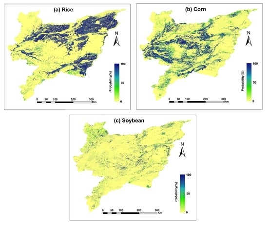
2.4. Crop Probability Maps Based on Optimized Feature Selection and Random Forest Classifier

As a natural nonlinear classifier, the Random Forest (RF) classifier uses multiple trees to train and predict samples, first proposed by Breiman [49]. A prominent advantage of the RF classifier is that it is less prone to overfitting and are more tolerant of noise and outliers [50]. The RF classifier mainly includes the following important parameters: (1) The number of trees in the forest. In theory, the more trees there are, the better the classification results, but at the same time, the classification time will increase. Therefore, we need to find a reasonable number of trees. Studies have shown that when the number of trees is more than 400, the OOB (out-of-bag) error of each classification situation tends to be stable [51]. In order to ensure the classification accuracy and reduce the computation time as much as possible, we set the number of trees to 500. (2) The total number of features, which was 77 in this study. (3) The maximum of features allowed in a decision tree in an RF algorithm. Generally, we took the square root of the total number of features as its value. In addition, in order to get better classification results, we set the recursive times to none and bootstrap (whether there is a sample returned) to true. The RF classifier for each crop was trained by using about half of the ground truth samples described in Section 2.2.2.

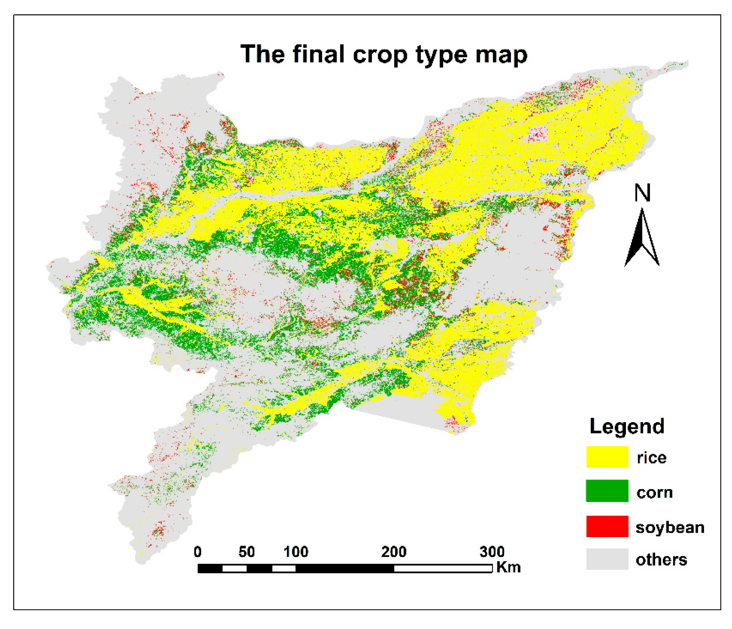
2.5. Final Crop Layer Based on the Combination of Three Crop Probability Maps

According to the obtained individual optimal feature sets of rice, corn, and soybean, we can input them into the RF classifier to make the probability maps. By compositing these three probability maps, we can obtain the final crop type map. Each pixel value in the final crop type map corresponds to one pixel in each of the three probability maps. By comparing the probabilities of the three pixels, if the pixel corresponding to the crop with the maximum probability has a probability value greater than 50%, it will be retained in the final crop type map. Otherwise, the pixel would be marked as “others”.

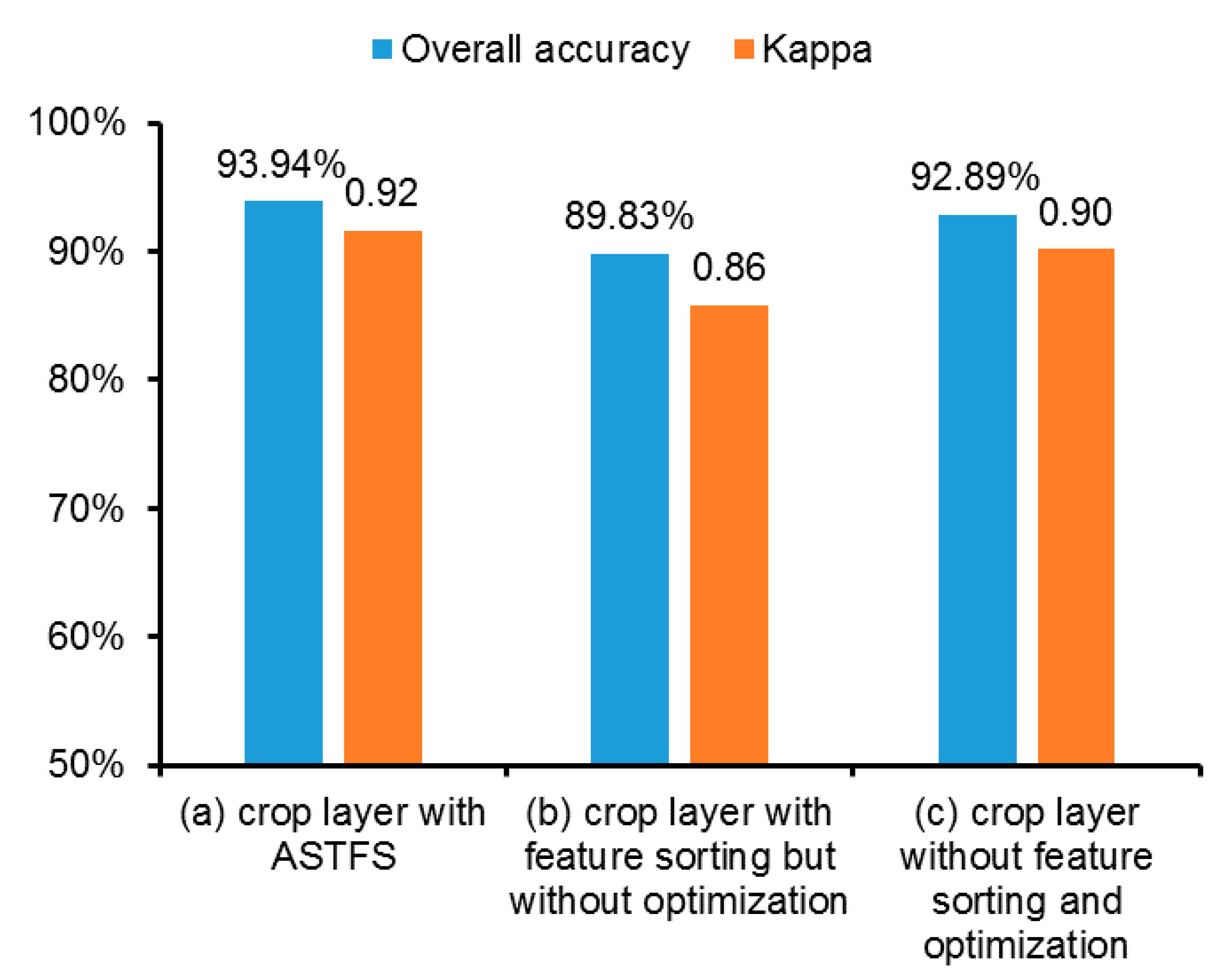
2.6. Accuracy Assessment and Comparison with Results from Unoptimized Features

In this study, the confusion matrix was used to validate the accuracy of all classification results based on 1996 ground object validation samples, which were kept apart from the training samples. The overall accuracy, producer’s accuracy, and user’s accuracy in the confusion matrix are important parameters for the accuracy assessment of classification results. The reliability of classification results is described from three different perspectives, which are most commonly used in land classification studies [52,53].
In order to represent the advantages of the ASTFS method in improving classification accuracy and efficiency, we also compared the classification result using optimal feature sets with two additional classifications using different input features as a part of accuracy assessment. The respective input feature sets of the two classifications are as follows: (1) All of the 77 spectro-temporal features (11 spectral indices or spectral bands multiplied 7 time points) for each of the three crops without feature optimization (“crop layer without feature sorting and optimization”), and (2) the same number of features with maximum global separability values as the number of optimal features (“crop layer with feature sorting but without optimization”). We made accuracy comparisons from two levels, accuracy comparisons for each crop (Section 3.2) and an overall accuracy comparison (Section 3.3) for three crops. The three classification feature sets were inputted into same Random Forest classifiers with the same parameter settings, classified with the same training dataset, and assessed with the same validation dataset.

3. Results

3.1. Spectro-Temporal Feature Analyses of Major Crops (Corn, Rice, and Soybean)

Figure 4 shows the average spectral curves of rice (black solid line), corn (black dotted line), soybean (black dashed line), and other ground objects (colored lines) in different spectral indices or bands, where the horizontal axes represent the months of crop growth in Sanjiang Plain (from April to October), and the vertical axes represent the vegetation indices or bands. Each spectral index corresponds to a certain physical and biological property of vegetation, and their regularity over time reflects the seasonal rhythms of crops [54,55]. It can be seen from Figure 4 that the spectral characteristics of corn, rice, and soybean in different vegetation indices or bands and at different time points are different, which also confirms the necessity of multi-spectral and multi-temporal images for crop identification.
As can be seen from Figure 4, there are strong similarities in the vegetation indices or band values of corn and soybean in many spectro-temporal features (for example, EVI from April to July, GCVI from April to August). This is because the corn and soybean in the Sanjiang Plain have similar growth processes and spectral characteristics, which greatly increases the difficulty of separating corn and soybean. However, band 8 in August, band 11 in July and August, and band 12 in July and August show potential to differentiate corn and soybean. Rice fields undergo sowing, flooding, and transplanting stages from about the end of April to the end of May (Figure 2), and the rice fields are covered by water during these three stages. Using this unique characteristic of rice, it is relatively easy to separate rice from other land covers.

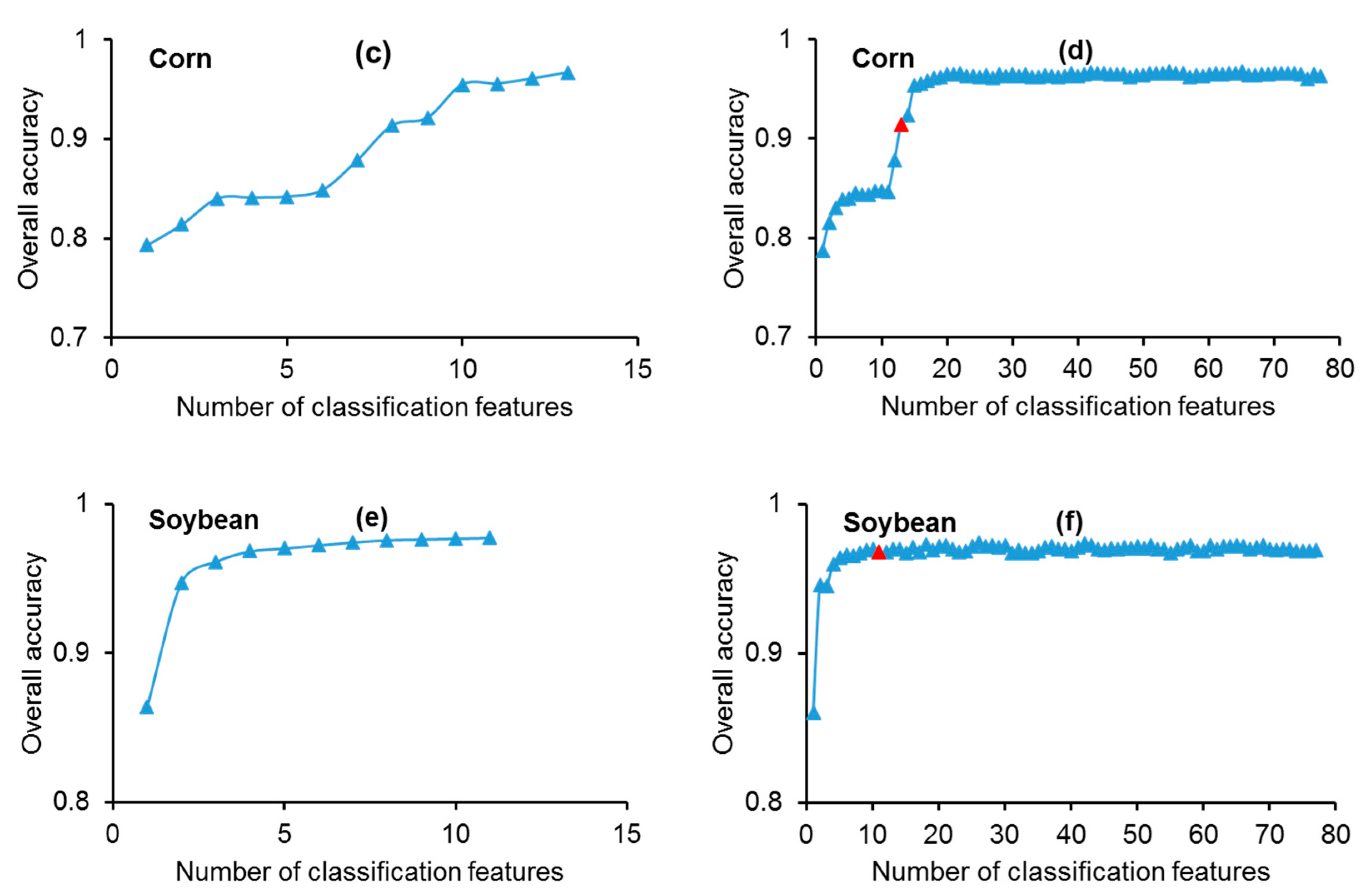
3.2. Feature Optimization Based on the ASTFS Method

The global separability indices for rice, corn, and soybean are shown in Figure 5 as the three global separability matrices. The horizontal axes represent seven temporal intervals from April to October, and the vertical axes represent 11 spectral indices and bands. The different colors of grids in these matrices represent the different values of the global separability index SIglobal. The colors of these grids vary from blue to red, which correspond to the values of SIglobal from low to high. Through the three global separability matrices in Figure 5, we obtained the importance ranking of all spectro-temporal features. It is clear from the three global separability matrices that the contribution of each spectro-temporal feature in classification is different. The classification accuracy will be reduced when the spectro-temporal feature with poor global separability is involved in the classification, which reflects the importance of feature selection optimization.
In terms of separating rice from other land cover classes, as shown in Figure 5a, the three spectral indices LSWI, NDSI, and NDSVI are the most important spectral features, and the three months April, May, and June are the most important temporal features. In the process of separating corn from other land cover classes, as shown in Figure 5b, the two vegetation indices LSWI and NDTI are the most important spectral features, and the two months May and June are the most important temporal features. In the process of separating soybean from other land cover classes, as shown in Figure 5c, the spectral index LSWI and the two bands 11 and 12 are the most important spectral features, and the three months May, June, and August are the most important temporal features.
The importance ranking of all spectro-temporal features for rice, corn, and soybean can be obtained based on the matrices. However, we could not input all available classification features to map crop type because the feature sets contained redundant or correlated information. Therefore, we removed the redundant features to reduce the curse of dimensionality in the classification (Figure 3). Finally, we obtained 22 optimal features for rice, 13 optimal features for corn, and 11 optimal features for soybean (Table 3).
According to the classification accuracies generated by the feature selection process, classification accuracy curves of individual optimal feature sets for rice, corn, and soybean were plotted (Figure 6a,c,e). In order to compare with the classification accuracy of optimal features, we compared classification accuracy for each crop, and classification accuracy curves of individual unoptimized feature sets (including all features in order of separability) for rice, corn, and soybean were also plotted (Figure 6b,d,f). The horizontal axes of the graphs in Figure 6 represent the number of classification features, while the vertical axes represent the overall accuracy of each classification. From Figure 6a,c,e, we can see that after removing redundant information, the classification accuracy improved as the number of classification features increased. Although we sorted all features according to their global separability from high to low, with the increase in the number of classification features, the classification accuracy did not increase in Figure 6b,d,f, but declined to a certain extent under the trend of overall increase. This is because there is redundant and correlated information between classification features. When information redundancy between features damages accuracy more than its contribution to accuracy, features redundancy is caused, which is called the "curse of dimensionality" [22,23]. The ASTFS method removes the redundant and correlated information contained in the feature set. By using the optimal classification features, the overall accuracies of individual rice, corn, and soybean probability maps were 99.15%, 96.69%, and 97.75%, respectively, which are the maximum in the three results. With the same number of features with maximum SIglobal values as the number of optimal features (the red triangles in Figure 6b,d,f), the classification accuracies only reached 98.25%, 91.33%, and 96.74%. Using all of the features of rice, corn, and soybean, their classification accuracies were 98.85%, 96.29%, and 96.89%. This just confirms the "curse of dimensionality" phenomenon mentioned above: Simply stacking many classification features will not improve the classification accuracy, but will cause information redundancy and reduce the classification accuracy.

3.3. Crop Mapping Based on Optimized Feature Selection and Accuracy Assessment

Based on the optimal feature sets for rice, corn, and soybean, as well as the Random Forest classifier, we generated the rice, corn, and soybean probability maps (Figure 7a–c). The final crop layer was generated by combining these three probability maps (Figure 8). Each pixel value in the final crop layer corresponds to the crop type with the maximum probability value. Figure 8 shows that crops are mainly located in the plain areas, excluding Wanda Mountain in the east, Changbai Mountain in the southwest, and Qinghei Mountain in the northwest of the Sanjiang Plain, which is consistent with the actual situation.
In order to evaluate the reliability of the resultant crop layer based on the ASTFS method, we compared it with another two results from (1) all of the 77 spectro-temporal features for each of the three crops without feature optimization (“crop layer without feature sorting and optimization”), and (2) the same number of features with maximum global separability values as the optimal features (“crop layer with feature sorting but without optimization”).
The three resultant crop type layers (crop layer with ASTFS, crop layer without feature sorting and optimization, and crop layer with feature sorting but without optimization) were validated by using the same ground truth samples (620 rice samples, 492 corn samples, 250 soybean samples, and 634 others samples). The comparison of overall accuracies and Kappa coefficients of the three crop type layers are shown in Figure 9, and the confusion matrices corresponding to individual classification results are shown in Table 4, Table 5 and Table 6. We found that the overall accuracy of the crop layer with ASTFS is 93.94% and the Kappa coefficient is 0.92, which is the maximum among the three results. For rice, the producer’s accuracy of the crop layer with ASTFS is 98.39% and the user’s accuracy is 98.07%, which is the maximum among the three results. Because of its unique phenological periods (e.g., flooding and transplanting stages), rice fields have special spectral characteristics. Therefore, rice is relatively easily distinguished from the three crops. For corn, the producer’s accuracy of the crop layer with ASTFS is 93.29% and the user’s accuracy is 92.73%, which is the maximum among the three results. For soybean, the producer’s accuracy of the crop layer with ASTFS is 82.00% and the user’s accuracy is 96.70%, which is the maximum among the three results. The reason why the producer’s accuracy of soybean is obviously lower than other accuracies in Table 4 is that some soybean fields are misclassified into corn and others. Soybean and corn have similar spectral characteristics and similar phenological periods, so it is difficult to distinguish between them. In addition, because the other types contain multiple land cover classes (forest, water, buildings, and other ground objects) and heterogeneity, some samples of rice, corn, and soybean are misclassified into others, and some others are also misclassified into the three crops. For others, the producer’s accuracy of the crop layer with ASTFS is 94.79% and the user’s accuracy is 90.10%, which is also the maximum among the three results. The analyses of classification results show that the ASTFS method is an effective feature selection method.

4. Discussion

4.1. Different Optimal Features for Identification of Rice, Corn, and Soybean

By using the ASTFS method, higher classification accuracy can be achieved with fewer classification features, also reducing computational complexity and time cost. In this study, we obtained three optimal feature sets for rice, corn, and soybean, which included 22, 13, and 11 features (Table 3), respectively. Specifically, we found that May and June are the most important phases to distinguish rice from other land cover classes, as rice undergoes flooding, transplanting, and reviving stages and the rice fields are covered by water in these periods. The corn and soybean fields are in the sowing stage and seeding stage (Figure 2), with low green vegetation and bare soil background in May and June. Differences in water content between rice fields and other types of farmlands caused their high pairwise separability in LSWI, NDSVI, and NDSI, which are sensitive to soil water content. Corn is also easily identified in May and June as it is in the sowing, seeding, three leaf, and seven leaf stages, while rice is in the flooding, transplanting, and reviving stages and soybean is in the sowing and seeding phases. In addition, the forest has higher vegetation coverage than corn in this period. In addition to May and June, August is another important time point to identify corn and soybean. Due to the similar spectral characteristics and phenological phases of corn and soybean, it is challenging to distinguish them [56,57]. According to Figure 2, corn enters the mature stage before soybean in August, which is an important phenological characteristic to distinguish corn from soybean. In the optimal features of soybean and corn, the short-wave infrared band in August is an important feature, which agrees with a previous study [40].

4.2. Implications of the ASTFS Method for Land Cover Classification

In this study, we proposed the ASTFS method and applied it to the Sanjiang Plain (about 108,900 km2) in the northeast of Heilongjiang Province of China. The ASTFS method well balanced the relationship between spectral separability and information redundancy and generated high classification accuracy in the resultant crop map. In this study, the resultant crop layer maps using optimal feature sets of rice, corn, and soybean are better than that using the same number of features with maximum SIglobal, as well as that using all the 77 spectro-temporal features. The results indicate that there is redundant information that not only fails to improve the classification accuracy, but also increases the computational complexity and time cost, suggesting the importance of feature selection. The ASTFS method proposed in this study can be extended and tested in a larger area, such as Northeast China and monsoon Asia, and also other sensors like Landsat and MODIS [55,58,59,60]. The improved regional crop type maps can provide important input data for crop growth monitoring and crop yield forecasting [61,62,63].
Although the ASTFS method was used to obtain the optimal feature sets of rice, corn, and soybean and good classification results were obtained, the method could be improved from the four aspects. First, this study used SIij when calculating pairwise separability. Other indicators could be used to quantify the inter-class separability as well. Second, when calculating SIglobal, this study adopted the average values of the pairwise separability indices as SIglobal for each feature. However, other means of calculating SIglobal, such as the minimum or maximum of the SIij, the weighted average of the SIij, and the average of normalized SIij, could be tested to improve the ASTFS method in the future. Third, ASTFS is currently limited to dealing with a single cropping and does not consider the identification of double or triple cropping. In the future, the ASTFS method could consider integrating the phase segmentation strategy [64] and more phenological metrics [65] to solve the crop identification problem of double or triple cropping. Finally, due to the unavailability of Sentinel-2 surface reflectance (SR) data in China before 2019 in the GEE platform, we used top of atmosphere (TOA) reflectance in this study. In the future, with the availability of SR data in China and continuous improvements (e.g., inclusion of the atmospheric correction tool for Sentinel-2) of the GEE platform, the results of crop classification and crop maps could be further improved.

5. Conclusions

While increasing numbers of medium resolution satellite imagery and improved machine learning algorithms become available, feature selection has rarely been investigated systematically for crop mapping. In this study, we proposed the automatic spectro-temporal feature selection (ASTFS) method for optimal feature selection, targeting an improved crop mapping strategy. The optimal classification feature sets of rice, corn, and soybean were obtained based on the ASTFS method, and then used for crop type layer mapping in the Sanjiang Plain of Northeast China. We found that when rice was in the flooding and transplanting stage in May, it was easy to separate from other land cover classes. The important phenological phases of corn are the seeding stage, three leaves stage, seven leaves stage, and the mature stage, and the corresponding months are May, June, and August. In particular, the mature stage in August is an important phenological phase for distinguishing corn and soybean. The short-wave infrared band plays an important role in distinguishing corn and soybean. These findings are specific for the Sanjiang Plain and may be transferable to other regions with different cropping calendars. The probability maps for the three crop types were generated based on the individual optimal feature sets of rice, corn, and soybean, and then these three maps were composited to generate the final crop type layer in the Sanjiang Plain according to their probability values. The crop type layer based on the ASTFS method showed a higher accuracy (overall accuracy (OA) = 93.94%, Kappa coefficient = 0.92) than the other two crop type maps: (1) Crop layer with feature sorting but without optimization (OA = 89.83%, and Kappa = 0.86), and (2) crop layer without feature sorting and optimization (OA = 92.89%, and Kappa = 0.90). With the same number of features, the classification accuracy of the crop layer with the ASTFS method is obviously better than the crop layer with feature sorting but without optimization. Although the classification accuracy of the crop layer with the ASTFS method is slightly better than the crop layer without feature sorting and optimization, the latter uses all features, which would greatly increase computational complexity and time cost. Through comparison, we confirmed that the ASTFS method is an effective feature optimization method for the extraction of rice, corn, and soybean in the Sanjiang Plain. The encouraging results from this study indicate that the ASTFS method has the potential to be used for the classification of crops or general land cover types and can be extensively applied for larger areas and using other sensors.

Author Contributions

G.Z., L.Y., J.H., and J.D. conceived and designed the experiments; L.Y. and N.Y. performed the experiments; L.Y. wrote the initial draft; and N.Y., G.Z., J.D., and J.H. analyzed the data and edited the paper. All authors have read and agreed to the published version of the manuscript.

Funding

This study was supported by the National Natural Science Foundation of China (Grant No. 41871349, 41671418, and 41971383), the Strategic Priority Research Program (XDA19040301), the Key Research Program of Frontier Sciences (QYZDB-SSW-DQC005) of the Chinese Academy of Sciences (CAS), and the “Thousand Youth Talents Plan”.

Acknowledgments

The authors thank Mrinal Singha, Arifuzzaman Khondakar, Tong Yang, and Yuanyuan Di for their valuable comments on the initial draft.

Conflicts of Interest

The authors declare no conflict of interest.

References

  1. Song, X.-P.; Potapov, P.V.; Krylov, A.; King, L.; Di Bella, C.M.; Hudson, A.; Khan, A.; Adusei, B.; Stehman, S.V.; Hansen, M.C. National-scale soybean mapping and area estimation in the United States using medium resolution satellite imagery and field survey. Remote Sens. Environ. 2017, 190, 383–395. [Google Scholar] [CrossRef]
  2. Prasad, A.K.; Chai, L.; Singh, R.P.; Kafatos, M. Crop yield estimation model for Iowa using remote sensing and surface parameters. Int. J. Appl. Earth Obs. 2006, 8, 26–33. [Google Scholar] [CrossRef]
  3. Biradar, C.M.; Thenkabail, P.S.; Noojipady, P.; Li, Y.; Dheeravath, V.; Turral, H.; Velpuri, M.; Gumma, M.K.; Gangalakunta, O.R.P.; Cai, X.L.; et al. A global map of rainfed cropland areas (GMRCA) at the end of last millennium using remote sensing. Int. J. Appl. Earth Obs. 2009, 11, 114–129. [Google Scholar] [CrossRef]
  4. Yang, N.; Liu, D.Y.; Feng, Q.L.; Xiong, Q.; Zhang, L.; Ren, T.W.; Zhao, Y.Y.; Zhu, D.H.; Huang, J.X. Large-Scale Crop Mapping Based on Machine Learning and Parallel Computation with Grids. Remote Sens. 2019, 11, 1500. [Google Scholar] [CrossRef] [Green Version]
  5. Jiang, H.; Li, D.; Jing, W.L.; Xu, J.H.; Huang, J.X.; Yang, J.; Chen, S.S. Early Season Mapping of Sugarcane by Applying Machine Learning Algorithms to Sentinel-1A/2 Time Series Data: A Case Study in Zhanjiang City, China. Remote Sens. 2019, 11, 861. [Google Scholar] [CrossRef] [Green Version]
  6. Zhang, J.C.; He, Y.H.; Yuan, L.; Liu, P.; Zhou, X.F.; Huang, Y.B. Machine Learning-Based Spectral Library for Crop Classification and Status Monitoring. Agronomy (Basel) 2019, 9, 496. [Google Scholar] [CrossRef] [Green Version]
  7. Deng, H.; Wang, D.; Liu, J.; Wang, L.; Chen, Z.; Zhou, Q.; IEEE. Extraction of Linear Surface Features from Remote Sensing Image to Construction Crop Acreage Survey Sampling Frame. In Proceedings of the 2011 IEEE International Geoscience and Remote Sensing, Vancouver, BC, Canada, 24–29 July 2011; pp. 2947–2948. [Google Scholar]
  8. Frogbrook, Z.L.; Oliver, M.A.; Salahi, M.; Ellis, R.H. Exploring the spatial relations between cereal yield and soil chemical properties and the implications for sampling. Soil Use Manag. 2002, 18, 1–9. [Google Scholar] [CrossRef]
  9. Pal, M.; Mather, P.M. An assessment of the effectiveness of decision tree methods for land cover classification. Remote Sens. Environ. 2003, 86, 554–565. [Google Scholar] [CrossRef]
  10. Pena-Barragan, J.M.; Ngugi, M.K.; Plant, R.E.; Six, J. Object-based crop identification using multiple vegetation indices, textural features and crop phenology. Remote Sens. Environ. 2011, 115, 1301–1316. [Google Scholar] [CrossRef]
  11. Yang, Z.; Shao, Y.; Li, K.; Liu, Q.; Liu, L.; Brisco, B. An improved scheme for rice phenology estimation based on time-series multispectral HJ-1A/B and polarimetric RADARSAT-2 data. Remote Sens. Environ. 2017, 195, 184–201. [Google Scholar] [CrossRef]
  12. Chang, J.; Hansen, M.C.; Pittman, K.; Carroll, M.; DiMiceli, C. Corn and soybean mapping in the united states using MODN time-series data sets. Agron. J. 2007, 99, 1654–1664. [Google Scholar] [CrossRef]
  13. Pan, Y.; Li, L.; Zhang, J.; Liang, S.; Zhu, X.; Sulla-Menashe, D. Winter wheat area estimation from MODIS-EVI time series data using the Crop Proportion Phenology Index. Remote Sens. Environ. 2012, 119, 232–242. [Google Scholar] [CrossRef]
  14. Hu, Q.; Wu, W.-B.; Song, Q.; Lu, M.; Chen, D.; Yu, Q.-Y.; Tang, H.-J. How do temporal and spectral features matter in crop classification in Heilongjiang Province, China? J. Integr. Agric. 2017, 16, 324–336. [Google Scholar] [CrossRef]
  15. Beeri, O.; Peled, A. Spectral indices for precise agriculture monitoring. Int. J. Remote Sens. 2006, 27, 2039–2047. [Google Scholar] [CrossRef]
  16. Song, Q.; Hu, Q.; Zhou, Q.; Hovis, C.; Xiang, M.; Tang, H.; Wu, W. In-Season Crop Mapping with GF-1/WFV Data by Combining Object-Based Image Analysis and Random Forest. Remote Sens. 2017, 9, 1184. [Google Scholar] [CrossRef] [Green Version]
  17. Zhang, J.; Feng, L.; Yao, F. Improved maize cultivated area estimation over a large scale combining MODIS-EVI time series data and crop phenological information. Isprs J. Photogramm. Remote Sens. 2014, 94, 102–113. [Google Scholar] [CrossRef]
  18. Foerster, S.; Kaden, K.; Foerster, M.; Itzerott, S. Crop type mapping using spectral-temporal profiles and phenological information. Comput. Electron. Agric. 2012, 89, 30–40. [Google Scholar] [CrossRef] [Green Version]
  19. Liu, Y.; Song, W.; Deng, X. Spatiotemporal Patterns of Crop Irrigation Water Requirements in the Heihe River Basin, China. Water 2017, 9, 616. [Google Scholar] [CrossRef] [Green Version]
  20. Xiao, X.M.; Boles, S.; Frolking, S.; Li, C.S.; Babu, J.Y.; Salas, W.; Moore, B. Mapping paddy rice agriculture in South and Southeast Asia using multi-temporal MODIS images. Remote Sens. Environ. 2006, 100, 95–113. [Google Scholar] [CrossRef]
  21. Zhong, L.; Gong, P.; Biging, G.S. Efficient corn and soybean mapping with temporal extendability: A multi-year experiment using Landsat imagery. Remote Sens. Environ. 2014, 140, 1–13. [Google Scholar] [CrossRef]
  22. Carrao, H.; Goncalves, P.; Caetano, M. Contribution of multispectral and multiternporal information from MODIS images to land cover classification. Remote Sens. Environ. 2008, 112, 986–997. [Google Scholar] [CrossRef]
  23. Loew, F.; Michel, U.; Dech, S.; Conrad, C. Impact of feature selection on the accuracy and spatial uncertainty of per-field crop classification using Support Vector Machines. Isprs J. Photogramm. Remote Sens. 2013, 85, 102–119. [Google Scholar] [CrossRef]
  24. Huang, J.; Hou, Y.; Wu, H.; Liu, J.; Zhu, D. Crop Type Mapping Method Based on Time-series MODIS Data in Heilongjiang Province. Trans. Chin. Soc. Agric. Mach. 2017, 48, 142–147, 285. [Google Scholar]
  25. Camps-Valls, G.; Mooij, J.; Schoelkopf, B. Remote Sensing Feature Selection by Kernel Dependence Measures. Ieee Geosci. Remote Sens. Lett. 2010, 7, 587–591. [Google Scholar] [CrossRef] [Green Version]
  26. Hu, Q.; Sulla, D.; Xu, B.D.; Yin, H.; Tang, H.J.; Yang, P.; Wu, W.B. A phenology-based spectral and temporal feature selection method for crop mapping from satellite time series. Int. J. Appl. Earth Obs. 2019, 80, 218–229. [Google Scholar] [CrossRef]
  27. Hu, Q.; Wu, W.; Song, Q.; Yu, Q.; Lu, M.; Yang, P.; Tang, H.; Long, Y. Extending the Pairwise Separability Index for Multicrop Identification Using Time-Series MODIS Images. Ieee Trans. Geosci. Remote Sens. 2016, 54, 6349–6361. [Google Scholar] [CrossRef]
  28. Zhao, Q.; Brocks, S.; Lenz-Wiedemann, V.I.S.; Miao, Y.; Zhang, F.; Bareth, G. Detecting spatial variability of paddy rice yield by combining the DNDC model with high resolution satellite images. Agric. Syst. 2017, 152, 47–57. [Google Scholar] [CrossRef]
  29. Onojeghuo, A.O.; Blackburn, G.A.; Wang, Q.; Atkinson, P.M.; Kindred, D.; Miao, Y. Mapping paddy rice fields by applying machine learning algorithms to multi-temporal Sentinel-1A and Landsat data. Int. J. Remote Sens. 2018, 39, 1042–1067. [Google Scholar] [CrossRef] [Green Version]
  30. Qin, Y.; Xiao, X.; Dong, J.; Zhou, Y.; Zhu, Z.; Zhang, G.; Du, G.; Jin, C.; Kou, W.; Wang, J.; et al. Mapping paddy rice planting area in cold temperate climate region through analysis of time series Landsat 8 (OLI), Landsat 7 (ETM+) and MODIS imagery. Isprs J. Photogramm. Remote Sens. 2015, 105, 220–233. [Google Scholar] [CrossRef] [Green Version]
  31. Zhang, G.; Xiao, X.; Dong, J.; Kou, W.; Jin, C.; Qin, Y.; Zhou, Y.; Wang, J.; Menarguez, M.A.; Biradar, C. Mapping paddy rice planting areas through time series analysis of MODIS land surface temperature and vegetation index data. Isprs J. Photogramm. Remote Sens. 2015, 106, 157–171. [Google Scholar] [CrossRef] [Green Version]
  32. Emelyanova, I.; Barron, O.; Alaibakhsh, M. A comparative evaluation of arid inflow-dependent vegetation maps derived from LANDSAT top-of-atmosphere and surface reflectances. Int. J. Remote Sens. 2018, 39, 6607–6630. [Google Scholar] [CrossRef]
  33. Xiong, J.; Thenkabail, P.S.; Tilton, J.C.; Gumma, M.K.; Teluguntla, P.; Oliphant, A.; Congalton, R.G.; Yadav, K.; Gorelick, N. Nominal 30-m Cropland Extent Map of Continental Africa by Integrating Pixel-Based and Object-Based Algorithms Using Sentinel-2 and Landsat-8 Data on Google Earth Engine. Remote Sens. 2017, 9, 1065. [Google Scholar] [CrossRef] [Green Version]
  34. Hao, P.Y.; Chen, Z.X.; Tang, H.J.; Li, D.D.; Li, H. New Workflow of Plastic-Mulched Farmland Mapping using Multi-Temporal Sentinel-2 data. Remote Sens. 2019, 11, 1353. [Google Scholar] [CrossRef] [Green Version]
  35. Goldblatt, R.; Stuhlmacher, M.F.; Tellman, B.; Clinton, N.; Hanson, G.; Georgescu, M.; Wang, C.Y.; Serrano-Candela, F.; Khandelwal, A.K.; Cheng, W.H.; et al. Using Landsat and nighttime lights for supervised pixel-based image classification of urban land cover. Remote Sens. Environ. 2018, 205, 253–275. [Google Scholar] [CrossRef]
  36. Jin, Z.N.; Azzari, G.; You, C.; Di Tommaso, S.; Aston, S.; Burke, M.; Lobell, D.B. Smallholder maize area and yield mapping at national scales with Google Earth Engine. Remote Sens. Environ. 2019, 228, 115–128. [Google Scholar] [CrossRef]
  37. Teluguntla, P.; Thenkabail, P.S.; Oliphant, A.; Xiong, J.; Gumma, M.K.; Congalton, R.G.; Yadav, K.; Huete, A. A 30-m landsat-derived cropland extent product of Australia and China using random forest machine learning algorithm on Google Earth Engine cloud computing platform. Isprs J. Photogramm. Remote Sens. 2018, 144, 325–340. [Google Scholar] [CrossRef]
  38. Zhang, X.; Wu, B.F.; Ponce-Campos, G.E.; Zhang, M.; Chang, S.; Tian, F.Y. Mapping up-to-Date Paddy Rice Extent at 10 M Resolution in China through the Integration of Optical and Synthetic Aperture Radar Images. Remote Sens. 2018, 10, 1200. [Google Scholar] [CrossRef] [Green Version]
  39. Wang, L.; Liu, J.; Yang, F.; Yao, B.; Jie, S.; Yang, L. Rice recognition ability basing on GF-1 multi-temporal phases combined with near infrared data. Trans. Chin. Soc. Agric. Eng. 2017, 33, 196–202. [Google Scholar]
  40. Wang, L.; Liu, J.; Yang, L.; Yang, F.; Fu, C. Impact of short infrared wave band on identification accuracy of corn and soybean area. Trans. Chin. Soc. Agric. Eng. 2016, 32, 169–178. [Google Scholar]
  41. Gitelson, A.A.; Vina, A.; Arkebauer, T.J.; Rundquist, D.C.; Keydan, G.; Leavitt, B. Remote estimation of leaf area index and green leaf biomass in maize canopies. Geophys. Res. Lett. 2003, 30. [Google Scholar] [CrossRef] [Green Version]
  42. Hao, P.; Zhan, Y.; Wang, L.; Niu, Z.; Shakir, M. Feature Selection of Time Series MODIS Data for Early Crop Classification Using Random Forest: A Case Study in Kansas, USA. Remote Sens. 2015, 7, 5347–5369. [Google Scholar] [CrossRef] [Green Version]
  43. Gao, B.C. NDWI - A normalized difference water index for remote sensing of vegetation liquid water from space. Remote Sens. Environ. 1996, 58, 257–266. [Google Scholar] [CrossRef]
  44. Friedl, M.A.; McIver, D.K.; Hodges, J.C.F.; Zhang, X.Y.; Muchoney, D.; Strahler, A.H.; Woodcock, C.E.; Gopal, S.; Schneider, A.; Cooper, A.; et al. Global land cover mapping from MODIS: Algorithms and early results. Remote Sens. Environ. 2002, 83, 287–302. [Google Scholar] [CrossRef]
  45. Klein, A.G.; Hall, D.K.; Riggs, G.A. Improving snow cover mapping in forests through the use of a canopy reflectance model. Hydrol. Process. 1998, 12, 1723–1744. [Google Scholar] [CrossRef]
  46. Wardlow, B.D.; Egbert, S.L. Large-area crop mapping using time-series MODIS 250 m NDVI data: An assessment for the US Central Great Plains. Remote Sens. Environ. 2008, 112, 1096–1116. [Google Scholar] [CrossRef]
  47. Somers, B.; Asner, G.P. Multi-temporal hyperspectral mixture analysis and feature selection for invasive species mapping in rainforests. Remote Sens. Environ. 2013, 136, 14–27. [Google Scholar] [CrossRef]
  48. Zhang, J.; Rivard, B.; Sánchez-Azofeifa, A.; Castro-Esau, K. Intra- and inter-class spectral variability of tropical tree species at La Selva, Costa Rica: Implications for species identification using HYDICE imagery. Remote Sens. Environ. 2006, 105, 129–141. [Google Scholar] [CrossRef]
  49. Breiman, L. Random forests. Mach Learn 2001, 45, 5–32. [Google Scholar] [CrossRef] [Green Version]
  50. Khosravi, I.; Alavipanah, S.K. A random forest-based framework for crop mapping using temporal, spectral, textural and polarimetric observations. Int. J. Remote Sens. 2019, 40, 7221–7251. [Google Scholar] [CrossRef]
  51. van Beijma, S.; Comber, A.; Lamb, A. Random forest classification of salt marsh vegetation habitats using quad-polarimetric airborne SAR, elevation and optical RS data. Remote Sens. Environ. 2014, 149, 118–129. [Google Scholar] [CrossRef]
  52. Foody, G.M. Status of land cover classification accuracy assessment. Remote Sens. Environ. 2002, 80, 185–201. [Google Scholar] [CrossRef]
  53. Liu, C.; Frazier, P.; Kumar, L. Comparative assessment of the measures of thematic classification accuracy. Remote Sens. Environ. 2007, 107, 606–616. [Google Scholar] [CrossRef]
  54. Johnson, D.M. An assessment of pre- and within-season remotely sensed variables for forecasting corn and soybean yields in the United States. Remote Sens. Environ. 2014, 141, 116–128. [Google Scholar] [CrossRef]
  55. De Petris, S.; Boccardo, P.; Borgogno-Mondino, E. Detection and characterization of oil palm plantations through MODIS EVI time series. Int. J. Remote Sens. 2019, 40, 7297–7311. [Google Scholar] [CrossRef]
  56. Chen, D.Y.; Huang, J.F.; Jackson, T.J. Vegetation water content estimation for corn and soybeans using spectral indices derived from MODIS near- and short-wave infrared bands. Remote Sens. Environ. 2005, 98, 225–236. [Google Scholar] [CrossRef]
  57. Johnson, D.M. Using the Landsat archive to map crop cover history across the United States. Remote Sens. Environ. 2019, 232. [Google Scholar] [CrossRef]
  58. Wulder, M.A.; Masek, J.G.; Cohen, W.B.; Loveland, T.R.; Woodcock, C.E. Opening the archive: How free data has enabled the science and monitoring promise of Landsat. Remote Sens. Environ. 2012, 122, 2–10. [Google Scholar] [CrossRef]
  59. Dong, J.; Xiao, X.; Menarguez, M.A.; Zhang, G.; Qin, Y.; Thau, D.; Biradar, C.; Moore, B., III. Mapping paddy rice planting area in northeastern Asia with Landsat 8 images, phenology-based algorithm and Google Earth Engine. Remote Sens. Environ. 2016, 185, 142–154. [Google Scholar] [CrossRef] [Green Version]
  60. Wardlow, B.D.; Egbert, S.L.; Kastens, J.H. Analysis of time-series MODIS 250 m vegetation index data for crop classification in the US Central Great Plains. Remote Sens. Environ. 2007, 108, 290–310. [Google Scholar] [CrossRef] [Green Version]
  61. Zhuo, W.; Huang, J.; Li, L.; Zhang, X.; Ma, H.; Gao, X.; Huang, H.; Xu, B.; Xiao, X. Assimilating Soil Moisture Retrieved from Sentinel-1 and Sentinel-2 Data into WOFOST Model to Improve Winter Wheat Yield Estimation. Remote Sens. 2019, 11, 1618. [Google Scholar] [CrossRef] [Green Version]
  62. Huang, J.; Gómez-Dans, J.L.; Huang, H.; Ma, H.; Wu, Q.; Lewis, P.E.; Liang, S.; Chen, Z.; Xue, J.-H.; Wu, Y.; et al. Assimilation of remote sensing into crop growth models: Current status and perspectives. Agric. For. Meteorol. 2019, 276–277, 107609. [Google Scholar] [CrossRef]
  63. Huang, J.; Zhuo, W.; Li, Y.; Huang, R.; Sedano, F.; Su, W.; Dong, J.; Tian, L.; Huang, Y.; Zhu, D.; et al. Comparison of three remotely sensed drought indices for assessing the impact of drought on winter wheat yield. Int. J. Digit. Earth. 2018, 1–23. [Google Scholar] [CrossRef]
  64. Conrad, C.; Colditz, R.R.; Dech, S.; Klein, D.; Vlek, P.L.G. Temporal segmentation of MODIS time series for improving crop classification in Central Asian irrigation systems. Int. J. Remote Sens. 2011, 32, 8763–8778. [Google Scholar] [CrossRef]
  65. Arvor, D.; Jonathan, M.; Penello Meirelles, M.S.; Dubreuil, V.; Durieux, L. Classification of MODIS EVI time series for crop mapping in the state of Mato Grosso, Brazil. Int. J. Remote Sens. 2011, 32, 7847–7871. [Google Scholar] [CrossRef]
Figure 1. The location of the study area and distribution of the ground truth sampling data.
Remotesensing 12 00162 g001
Figure 2. Crop calendars for the three major crops (corn, rice, and soybean) in the Sanjiang Plain [30,31]. We divided a month into three parts (e.g., early April (E), middle April (M), and late April (L)). Rice: 1, sowing; 2, seeding/flooding; 3, transplanting; 4, reviving; 5, tillering; 6, booting; 7, heading; 8, milk stage; 9, mature; and 10, harvest; Corn: 1, sowing; 2, seeding/three leaves; 3, seven leaves; 4, stem elongation; 5, heading; 6, milk stage; 7, mature; and 8, harvest; Soybean: 1, sowing; 2, seeding; 3, the third true leaf; 4, flowing; 5, pod setting; 6, mature; and 7, harvest.
Remotesensing 12 00162 g002
Figure 3. The workflow of the automatic spectro-temporal feature selection (ASTFS) method for selecting the optimal features for certain crop type. RF, Random Forest.
Remotesensing 12 00162 g003
Figure 4. Time series profiles of major crops (corn, rice, and soybean) and other land cover classes (forest, water, built-up land, and others) for 11 vegetation indices and three bands. Panels from (a) to (k) represent EVI, GCVI, LSWI, NDSI, NDSVI, NDTI, NDVI, NDWI, band 8, band 11, and band 12, respectively. The horizontal and vertical axes refer to the month of year and the spectral index or band values, respectively.
Remotesensing 12 00162 g004
Figure 5. SIglobal pattern for identifying rice alone (a), corn alone (b), and soybean alone (c).
Remotesensing 12 00162 g005
Figure 6. Classification accuracy curves of individual optimal (a,c,e) and unoptimized (b,d,f) feature sets for rice, corn, and soybean. The red triangles in (b,d,f) correspond to the same number of features with the maximum global separability values as the number of optimal features (a,c,e).
Remotesensing 12 00162 g006aRemotesensing 12 00162 g006b
Figure 7. (a) Rice probability map with optimized features for rice. (b) Corn probability map with optimized features for corn. (c) Soybean probability map with optimized features for soybean.
Remotesensing 12 00162 g007
Figure 8. Crop map based on the probability map of corn, rice, and soybean based on optimized feature selection.
Remotesensing 12 00162 g008
Figure 9. Comparisons of overall accuracies and Kappa coefficients of resultant (a) crop layer with ASTFS (using 22 optimal features for rice, 13 optimal features for corn, and 11 optimal features for soybean), (b) crop layer with feature sorting but without optimization (using 22 features for rice, 13 features for corn, and 11 features for soybean), and (c) crop layer without feature sorting and optimization (using individual 77 features for rice, corn, and soybean).
Remotesensing 12 00162 g009
Table 1. A summary of vegetation indices in classification feature set, including their spectral regions, computational formulas, associated vegetation properties, and references.
Spectral RegionVegetation Index FormulaCommonly Related toAssociated Reference
Visible-NIRNDWI B 3 B 8 B 3 + B 8 Vegetation phenology, vegetation photosynthetic activity, land cover[43]
NIR-VisibleNDVI B 8 B 4 B 8 + B 4 Vegetation growth status, vegetation coverage[44]
SWIR–SWIRNDTI B 11 B 12 B 11 + B 12 Non-photosynthetic components, residue cover[21]
Visible-SWIRNDSVI B 11 B 4 B 11 + B 4 Vegetation status, water content, residue cover[21]
Visible-SWIRNDSI B 3 B 11 B 3 + B 11 Snow cover[45]
NIR–SWIRLSWI B 8 B 11 B 8 + B 11 Water content, residue cover[20]
NIR-VisibleGCVI B 8 B 3 1 Chlorophyll content[41]
Visible-NIREVI 2.5 × B 8 B 4 B 8 + 6 × B 4 + 7.5 + B 2 + 1 Vegetation status, canopy structure[46]
Table 2. A summary of bands in classification feature set, including their central wavelength, bandwidth, and spatial resolutions.
Sentinel-2ASentinel-2B
Band NumberCentral Wavelength (nm)Bandwidth (nm)Central Wavelength (nm)Bandwidth (nm)Spatial Resolution (m)
8832.8106833.010610
111613.7911610.49420
122202.41752185.718520
Table 3. Individual optimal features for rice, corn, and soybean selected by the ASTFS method.
Crop TypeOptimal Features
RiceNDSI, May; NDSI, June; LSWI, May; NDSVI, June; band 11, June; LSWI, June; NDSI, Apr.; band 11, Apr.; band 12, June; band 11, July; NDSI, Aug.; NDTI, May; NDSI, Sept.; band 12, June; band 8, May; NDWI, Apr.; NDVI, Apr.; NDWI, June; band 8, Oct.; band8, Sept.; NDWI, Sept.; GCVI, Sept.
CornLSWI, May; LSWI, June; NDTI, May; band 12, June; LSWI, Apr.; NDTI, Apr.; NDTI, Aug.; NDSI, June; EVI, Aug.; band 11, Aug.; band 8, Aug.; band 12, Aug.; band 11, July
SoybeanLSWI, May; band 11, Aug.; band 12, Aug.; band 11, July; band 12, June;
NDSI, Aug.; band 12, July; band 8, Aug.; NDTI, Apr.; LSWI, Apr.; band 11, May
Table 4. Confusion matrix of crop layer with ASTFS.
Classified DataRiceCornSoybeanOthersProducer’s Accuracy (%)
Reference Data
Rice61020898.39%
Corn045933093.29%
Soybean0172052882.00%
Others1217460194.79%
User’s accuracy (%)98.07%92.73%96.70%90.10%
Table 5. Confusion matrix of crop layer with feature sorting but without optimization.
Classified DataRiceCornSoybeanOthersProducer’s Accuracy (%)
Reference Data
Rice604101597.42%
Corn041227883.74%
Soybean0441802672.00%
Others1911759794.16%
User’s accuracy (%) 96.95% 88.03% 95.24% 83.38%
Table 6. Confusion matrix of crop layer without feature sorting and optimization.
Classified DataRiceCornSoybeanOthersProducer’s Accuracy (%)
Reference Data
Rice60740997.90%
Corn045743192.89%
Soybean0141954178.00%
Others1420559593.85%
User’s accuracy (%)97.75% 92.32% 95.59% 88.02%

