Real-Time Uncertainty Specification of All Sky Imager Derived Irradiance Nowcasts

Abstract

The incoming downward shortwave solar irradiance is harvested to an increasing extent by solar power plants. However, the variable nature of this energy source poses an operational challenge for solar power plants and electrical grids. Intra hour solar irradiance nowcasts with a high temporal and spatial resolution could be used to tackle this challenge. All sky imager (ASI) based nowcasting systems fulfill the requirements in terms of temporal and spatial resolution. However, ASI nowcasts can only be used if the required accuracies for applications in solar power plants and electrical grids are fulfilled. Scalar error metrics, such as mean absolute deviation, root mean square deviation, and skill score are commonly used to estimate the accuracy of nowcasting systems. However, these overall error metrics represented by a single number per metric are neither suitable to determine the real time accuracy of a nowcasting system in the actual weather situation, nor suitable to describe any spatially resolved nowcast accuracy. The performance of ASI-based nowcasting systems is strongly related to the prevailing weather conditions. Depending on weather conditions, large discrepancies between the overall and current system uncertainties are conceivable. Furthermore, the nowcast accuracy varies strongly within the irradiance map as higher errors may occur at transient zones close to cloud shadow edges. In this paper, we present a novel approach for the spatially resolved real-time uncertainty specification of ASI-based nowcasting systems. The current irradiance conditions are classified in one of eight distinct temporal direct normal irradiance (DNI) variability classes. For each class and lead-time, an upper and lower uncertainty value is derived from historical data, which describes a coverage probability of 68.3%. This database of uncertainty values is based on deviations of the irradiance maps, compared to three reference pyrheliometers in Tabernas, Andalucia over two years (2016 and 2017). Increased uncertainties due to transient effects are considered by detecting transient zones close to cloud shadow edges within the DNI map. The width of the transient zones is estimated by the current average cloud height, cloud speed, lead-time, and Sun position. The final spatially resolved uncertainties are validated with three reference pyrheliometers, using a data set consisting of the entire year 2018. Furthermore, we developed a procedure based on the DNI temporal variability classes to estimate the expected average uncertainties of the nowcasting system at any geographical location. The novel method can also be applied for global tilted or horizontal irradiance and is assumed to improve the applicability of the ASI nowcasts.

1. Introduction

The main sources of intra hour and intra minute solar irradiance variability are clouds. Highly variable solar irradiance conditions pose a control challenge for solar thermal power plants and electrical grids of countries with a high solar penetration. All sky imager (ASI)-based nowcasting systems of solar irradiance, with their high temporal and spatial resolution, can be useful to tackle this control challenge [1,2]. In past years, various ASI-based nowcasting systems were developed. Some of these systems are based on a single ASI (e.g., [3,4]) while others are based on multiple ASIs (e.g., [5,6]). All ASI-based nowcasting systems need a cloud segmentation. Commonly used cloud segmentation approaches use machine learning (e.g., [7,8]) while others use fixed (e.g., [9,10]) or variable (e.g., [11]) thresholds. Further important processing steps for nowcasting systems are the cloud tracking (e.g., [12,13]) and an analysis of the current and future radiative effect (e.g., [14,15]) of the clouds. Cloud height is not needed if the nowcast targets only the area directly next to the ASI. However, when spatially resolved irradiance maps for larger areas are desired, the cloud height has to be known. Stereoscopic cloud height estimation approaches with multiple ASIs are often described in the literature (e.g., [16,17]).

Whether nowcasting systems can be used effectively for the control optimization of power plants and electrical grids depends to a large extent on their accuracies. Such delicate control applications (e.g., mass flow control in concentrating solar thermal power plants, ramp rate control in photovoltaic power plants, and load management in electrical grids) require a real time uncertainty specification in order to assess the obtained nowcasting information during operation and reject them if needed. Methods supporting increased robustness in using irradiance nowcasts are as important as increasing the accuracy of the nowcasting methods itself.

The root mean square deviation (RMSD) and the mean absolute deviation (MAD) are often used as error metrics for nowcasting systems (e.g., [18,19,20,21,22]). The mentioned studies use validation periods from 15 days to six months. The validation results represent the overall accuracy of the nowcasting systems within this period for the used site. As already discussed in other studies [23], nowcasting validation results are strongly influenced by the chosen data set and the prevailing weather conditions. [23] proposes the well-known meteorological concept of using skill scores s (see Equation (1)) as the main benchmarking metrics for nowcasting systems. The skill score s compares the RMSD of the nowcasting system (index N) with the corresponding RMSD of a persistence nowcast (index P).

$$s= 1-RMS{D}_N/RMS{D}_P,$$

(1)

As most other accuracy metrics, the skill score also depends on the used observations and the prevailing weather conditions during that period at the chosen geographical locations. This makes the comparison between different nowcasting systems, on the basis of published results using different observational data sets, complicated. The use of such previously published error quantification is, therefore, unsuitable as the real time uncertainty assessment.

In this study, we present a spatial real-time uncertainty specification approach for ASI-based nowcasts. The focus of this work is not the uncertainty/accuracy of the used nowcasting system itself, but the used methodology to identify spatial real time uncertainties of ASI–based nowcasting systems in general. For a real-time application, the methodology must be capable in determining appropriate uncertainties under all possible ambient conditions. The used nowcasting system itself had been benchmarked in previous publications [22,24]. In our study, the basis are DNI nowcasts, but the same approach can be applied for nowcasting global horizontal irradiance (GHI) or global tilted irradiance (GTI).

For the uncertainty specification of the nowcasting system, we classify the weather conditions at CIEMATs Plataforma Solar de Almería (PSA) over a 2-year period (2016 and 2017) by evaluating the DNI variability according to [25]. Over the same period, deviations of the nowcasting system compared to three spatial distributed pyrheliometers are analyzed and discretized in the DNI variability classes. A basic uncertainty is derived by evaluating the observed coverage probability of deviations within the DNI variability classes. Furthermore, we analyze the spatial effect of the expected uncertainty in more error prone transient zones of the DNI maps. The transient zones are defined as the potential area of cloud shadow edges, with strong alternations from sunny to shaded areas. However, the exact position of the cloud shadow edges is uncertain. Therefore, we estimate the expected uncertainty of the cloud shadow edge positions with previously obtained validation results of the used cloud height and cloud-tracking algorithm [26] and combine this with the basic uncertainty information. Hereby, a transient bandwidth is determined around the expected cloud shadow edges with increased uncertainties. The final nowcasting output consists of three distinct spatial DNI information: the actual nowcasted DNI as well as an upper and a lower limit. The upper and lower limits describe the DNI with uncertainty and a coverage probability of ~68.3%.

Various settings and image processing steps have an influence on the final nowcasting uncertainty. The main contributors to the uncertainty are the camera alignment and calibration, the cloud segmentation, modeling, tracking, and shadow projection. A clear separation of the individual uncertainty contributors is not possible. Yet, we present validation results of the uncertainty specification with a data set consisting of the entire year 2018. The validation is done with three reference pyrheliometers. We analyze the overall average coverage probability that reached with the allocated uncertainties.

Apart from the real-time specification of the nowcast uncertainties, the determined basic uncertainty can be used to compare the expected uncertainties of the same nowcasting system at different geographical sites with divergent weather conditions.

In Section 2, we introduce the nowcasting system for which the uncertainty maps are created. Section 3.1 presents the used DNI variability classification procedure. The uncertainty specification method itself is explained in Section 3.2. A comparison of the expected average uncertainties of the same nowcasting system at two distinct sites is performed in Section 3.3. Lastly, we conclude our findings in Section 4.

2. Materials

The nowcasting system uses a DNI measurement taken by a Kipp&Zonen CHP1 pyrheliometer (number 1, see Figure 1) and the images of two Mobotix Q24 surveillance cameras with fisheye lenses operated at the PSA. Corresponding metrological data of the pyrheliometer station 1 for the year 2016 as well as videos from both ASIs for an example day (14 May 2016) are available in the supplementary materials(see Video S1). The cameras are mounted 494 m apart from each other. The 3-mega pixel (MP) images are taken from the sky and converted into 1 MP orthogonal image with a maximum zenith angle of 78°. Two additional reference pyrheliometers (sensor number 2 and 3) are placed north of the cameras (see Figure 1). These additional pyrheliometers are used for the nowcast validation and uncertainty specification, with a data set including all the days of the years 2016 and 2017. A third additional pyrheliometer (number 4) is positioned next to ASI 1. This sensor is only used during the validation procedure of the specified uncertainties (see Section 3.2.3). The validation procedure uses a data set with all days of the year 2018. This fourth sensor is a substitution for pyrheliometer 3, since pyrheliometer 3 was not operated in 2018. The used instrumentation is cleaned each weekday and the DNI data are quality-screened, according to [27].

The nowcasting system uses a four dimensional clear sky library for the cloud segmentation [22,28] and a stereoscopic cloud geolocation and tracking approach [26]. The radiative effect of the detected clouds is analyzed by a probabilistic approach using current and historical cloud transmittance and cloud height measurements [24]. The nowcasting system creates DNI maps with edge lengths of 8 km and lead times up to 15 min ahead [29].

Kuhn et al. [22] presented a validation procedure for the nowcasting system based on three reference pyrheliometer. In [24], we presented the validation results according to [22], for the years 2016 and 2017. An overall RMSD, MAD, bias, and skill score of 21%, 13%, 5%, and 7% was reached for a lead-time of 10 min. However, these error metrics show only the overall deviations over the entire data set. Nevertheless, as mentioned before, the nowcasting performance strongly varies with the prevailing weather conditions. Especially highly variable complex multi-layer conditions lead to larger error metrics, compared to less variable low cloud altitude single-layer conditions (e.g., [24])

3. Methods and Results

3.1. Temporal DNI Variability Classes

For the determination of real time uncertainties, a variability classification of the most recent irradiance conditions is used. A classification method based on eight distinct variability classes for 1 min resolved DNI data on an hourly basis. This is introduced by [25,30]. The classes differ as follows:

• Class 1 describes clear sky conditions.
• Classes 2 and 3 describe nearly clear sky conditions with a stronger variability and comparatively lower average DNI in the case of class 3.
• Class 4 shows a strong temporal variability but with an overall high average DNI.
• Class 5 describes less variable conditions with a lower average DNI compared to class 4.
• Class 6 resembles class 4 with a strong temporal variability, but with a significantly lower average DNI.
• Class 7 describes nearly complete overcast situations with some ramps.
• Class 8 corresponds to overcast situations.

The classification procedure described in [25] uses 13 variability indices, which partially have been introduced in previous publications (see

Table 1. Variability indices used by [25].

Index	Description	Unit	Introduced by
CSFD	Number of changes in the sign of the first derivative	-	[31]
meankcDNI	Average of clear sky index kcDNI (clear sky DNI := cDNI)	-	[32]
ΔkcDNI_σ	$\Delta k_{cDNI}=\begin{array}{c}{k}_{cDNI}\left(i\right)-k_{cDNI}\left(i-1\right)\\ ⋮\\ k_{cDNI}\left(n\right)-k_{cDNI}\left(n-1\right)\end{array}$ $\sqrt{\frac{1}{n-1}{\displaystyle \sum _{i=1}^n}{\left(\Delta k_{cDNI,i}-{\overline{\Delta k}}_{cDNI}\right)}^2}$ Data sample i from data package with n data samples	-	[32]
ΔkcDNI_mean	${\displaystyle \sum _{i=1}^n}\Delta k_{cDNI,i}/n$	-	[32]
ΔkcDNI_max	$max\left(\Delta k_{cDNI}\right)$	-	[32]
ΔDNI_σ	$\Delta DNI=\begin{array}{c}DNI\left(i\right)-DNI\left(i-1\right)\\ ⋮\\ DNI\left(n\right)-DNI\left(n-1\right)\end{array}$ $\sqrt{\frac{1}{n-1}{\displaystyle \sum _{i=1}^n}{\left(\Delta DN{I}_i-\overline{\Delta DNI}\right)}^2}$	W/m2	[25]
ΔDNI_mean	${\displaystyle \sum _{i=1}^n}\left|\Delta DNI\right|/n$	W/m2	[25]
ΔDNI_max	$max\left(\left|\Delta DNI\right|\right)$	W/m2	[25]
VI_DNI	$VI=\frac{{{\displaystyle \sum }}_{i=2}^n\sqrt{{\left(DNI\left(i\right)-DNI\left(i-1\right)\right)}^2+\Delta t^2}}{{{\displaystyle \sum }}_{i=2}^n\sqrt{{\left(CSDNI\left(i\right)-CSDNI\left(i-1\right)\right)}^2+\Delta t^2}}$.	-	[33]
V_DNI	$V=\sqrt{\frac{1}{n}{\displaystyle \sum _{t=1}^n}{\left(\Delta k_c\right)}^2}$	-	[34]
Integral Upper Minus Lower (UML)	Envelope curves of DNI ${{\displaystyle \int }}^{}uppe{r}_{env}-lowe{r}_{env}$	J/m2	[30]
Integral Upper Minus Clear (UMC)	Envelope curves of DNI ${{\displaystyle \int }}^{}uppe{r}_{env}-CSDNI$	J/m2	[30]
Integral Lower Minus Abscissa (LMA)	Envelope curves of DNI ${{\displaystyle \int }}^{}lowe{r}_{env}$	J/m2	[30]

).

The classification is done by comparing these 13 normalized variability indices with corresponding typical values for each variability class and determining the class with the lowest distance metric to the mean of a reference probability density distribution of all variability classes. These probability densities are derived once using a manually classified reference data set [25].

This work uses the classification procedure described in [25] with a reduction of the evaluated time interval from one hour to 15 min to cope with the very high spatial and temporal resolution characteristics of the ASI-based nowcasting. Due to the reduction of the time interval from one hour to 15 min, the corresponding probability density functions for the variability indices of CSFD and LMA were linearly scaled down to a 15-min base (not required for the remaining indices).

The needed clear sky DNI is the most recent clear DNI measurements detected according to [35,36]. A temporal weighted averaged Linke turbidity is calculated from the most recent clear DNI values according to [37]. Subsequently, the clear sky DNI for the shaded time stamps is calculated with the current Linke turbidity according to [37].

The motivation for the reduced temporal resolution can be seen in Figure 2. The DNI of an example day, with highly variable and stable time windows, is depicted together with the clear sky DNI and the assigned variability class. A new assessment of the variability takes place with every new time stamp (1 min resolution), considering the prevailing DNI of the last 60 or 15 min. The 60-min approach is often too inert for an inter-hour consideration. This is particularly evident in the time windows from 11:54 to 12:38, 13:21 to 13:59, and 15:30 to 16:00, which show clear sky conditions. The 60-min approach reacts slower than the 15-min approach and misses completely the two clear windows from 13:21 to 13:59 and 15:30 to 16:00. The 15-min approach reacts 2 min after the start of the clear windows by moving toward class 1.

We analyze whether a single point like the DNI measurement (e.g., pyrheliometer) is meaningful to derive the variability class for an entire industrial size solar field of 2 km². We observe a perfect match of the selected variability class in 94.9% of all cases across a 30-day test period, comparing the classification based on a point like DNI measurement or the DNI field average derived from DNI maps. Therefore, we conclude that a single point like measurement is suitable to identify the variability class for the whole area of a large commercial solar field. More detailed results of this study are given in Appendix A.

3.2. Weather Dependent Uncertainty Specification

3.2.1. Determination of Uncertainties

Sky images of the complete years 2016 and 2017 are evaluated. The used nowcasting system creates 16 DNI maps for each image series with lead times up to 15 min ahead in 1-min increments. Pyrheliometer measurement from three reference sensors (number 1, 2 and 3 see Figure 1) are compared to the corresponding DNI values from the DNI maps. The derived deviation between the reference sensors and the nowcasting system is the basis for the uncertainty specification. The DNI variability is classified for each time stamp. We use the last 15 min of the DNI observation of one of the three reference pyrheliometer (sensor next to ASI 2, see Figure 1), according to the procedure described in Section 3.1. As already mentioned, the point like measurement of a single pyrheliometer is sufficiently adequate to classify the area around the three reference pyrheliometers and two ASIs placed to each other at a largest distance of 891 m. The nowcasted DNI with lead times > 0 min could be used for the DNI variability classification. However, this would mean that the yet unknown uncertainties of the nowcasting system would affect the DNI classification, which, in turn, serves as the basis of the uncertainty analysis. The use of the more accurate measured DNI signal of the past 15 min might cause a poorly defined uncertainty in the case of sudden atmospheric changes of the conditions, especially for high lead times, but this is only a short-term effect. As we discussed in Section 3.1, the DNI variability classification procedure on the basis of a 15-min time window, reacts rapidly on any changes of irradiance conditions. Furthermore, we will introduce (in Section 3.2.2) additional spatial adaptions within transient zones of the DNI maps, which reduce potential negative effects of the DNI variability classification with data from the recent past.

For the uncertainty specification, we calculate the average deviation $De{v}_i$ between the three spatially distributed reference pyrheliometers and the corresponding nowcasting DNI from the DNI maps for each time stamp i.

$$De{v}_i=\frac{{{\displaystyle \sum }}_{st=1}^3\left(DN{I}_{i,st,ref}-DN{I}_{i,st,nc}\right)}{3}$$

(2)

The index st describes the reference station number, ref the reference DNI, and nc, which is the corresponding nowcasted DNI. The resulting deviations for each image series are discretized over the DNI variability classes and two Sun elevation ranges (above and below 30°). The distribution of the deviations $De{v}_i$ over the entire data set is analyzed within each DNI variability class, Sun elevation range, and lead-time. Figure 3 shows the distribution within each DNI variability class and lead-time as a 2-D histogram with a logarithmic scale (Sun elevation angle above 30°). From the distribution within each DNI variability class, the upper (positive $De{v}_i$ values) and lower (negative $De{v}_i$ values) limits are detected, which frame a coverage probability of 68.3% (p68.3). These p68.3 values are marked as pink dashed lines in Figure 3. The discretization in two Sun elevation ranges above and below 30° is chosen due to notable deviation in p68.3 values in between these Sun elevation ranges. The results of a study, which compares p68.3 values within different Sun elevation ranges, is presented in Appendix B.

The p68.3 lower and upper range limits are saved in a look-up table, according to the DNI variability class, Sun elevation angle, and lead time (Figure 4). These values are considered as the basic uncertainty of the nowcasting system. In this manuscript, we use the terms u_up for the positive and u_low for the negative part of the uncertainty. Class 1 and class 2 show the narrowest range between u_up and u_low with almost no impact on the lead-time. The remaining classes show an increasing range with an increasing lead-time. This increase of the u_up and u_low range is particularly strong within the lead times of 0 to 4 min, starting with a range of ±100 W/m² or smaller for all classes. The widest u_up and u_low ranges are reached by the highly variable classes 4 and 6 as well as class 7 and a lead-time of 15 min. For the Sun elevation range above 30°, class 7 shows a pronounced bias toward negative deviations. This bias exists for the Sun elevation range below 30°, but is less pronounced. This indicates that the nowcasting system rather misses clouds than falsely detects a clear sky as cloud. From the look up table, it is clear that the presented nowcasting system can deliver accurate DNI information for the current situation and immediate intra-minute nowcasts. However, the uncertainties increase rapidly in the case of variable conditions and higher lead times. During the operation of the nowcasting system, the DNI variability is classified constantly with measurements of the pyrheliometer. The DNI variability class, Sun elevation angle, and lead-time from the look-up table shown in Figure 4 derived the expected basic uncertainty.

For some applications, intra-minute nowcasts could be of interest as e.g., in the aim point strategy of solar tower power plants [38]. As it can be seen in Figure 4, the uncertainties for lead times up to 1 min ahead and all DNI variability classes below ±150 W/m², for the presented nowcasting system.

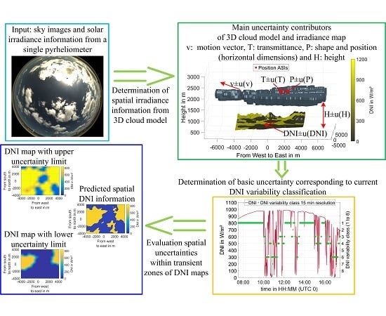
3.2.2. Real-Time Uncertainty Assessment of Spatial DNI Maps

The nowcasting system delivers for each time stamp and lead time for three distinct DNI maps including the standard DNI map without uncertainty, the DNI map with u_up basic uncertainty as the upper limit, and the DNI map with u_low basic uncertainty as a lower limit. A direct homogenous application of the basic uncertainty on the spatial DNI maps is not feasible. Corrections are necessary for some areas of the DNI map. On the one hand, there are physical boundaries. The DNI values of the DNI map cannot drop below 0 W/m² or surpass the current clear sky DNI. The u_up and u_low are adjusted in regions of the DNI map, where these physical boundaries would be surpassed. DNI values of these regions are set to 0 W/m² or to the current clear sky DNI, respectively. On the other hand, transition zones lead to a spatially limited increase of the uncertainties. These transition zones describe areas close to cloud shadow edges on the DNI maps. Erroneous shadow edge positions lead to large, spatially confined errors of the DNI magnitude, depending on the prevailing clear sky DNI and cloud transmittance for the corresponding DNI map pixel. Figure 5 illustrates the expected and possible alternative cloud edge position as well as the influence of uncertain cloud edge positions on the spatial DNI information around an arbitrary reference point.

For the nowcasting system, the main source of the false shadow positions are the cloud height detection and cloud tracking. [39] investigated the impact of the ideal camera distance for cloud height measurements with ASIs. The used setup with an ASI distance of roughly 494 m and orthogonal image resolution of 1MP (maximum zenith angle of 78°) is less suitable for cloud heights above 5000 m [39]. These results are in alignment with actual cloud height and tracking validation results of the used nowcasting system [26]. The overall results of the validation are presented in

Table 2. Validation results of ASI-based cloud height and cloud tracking approach over cloud height and cloud speed ranges for the selected multi-ASI configuration [26].

Cloud Height Range	MAD Cloud Height	Cloud Speed Range	MAD Cloud Speed
0–3000 m	312 m	0–6 m/s	1.33 m/s
3000–6000 m	996 m	6–12 m/s	1.92 m/s
6000–9000 m	2665 m	12–18 m/s	2.52 m/s
9000–12,000 m	2431 m

, discretized over cloud height and cloud speed ranges. The increase of the deviations for higher cloud height ranges and cloud speed ranges is due to the used ASI setup and the chosen resolution. For the cloud movement directions, an overall MAD of 12.8° was determined.

The impact of an uncertain cloud height on the cloud shadow position depends on the Sun elevation angle. Lower Sun elevation angles lead to more pronounced uncertainties of the cloud shadow position. This effect is illustrated in Figure 6.

The influence of an erroneous cloud speed on a false cloud shadow position increases with lead-time. Figure 7 shows the expected uncertainties on the cloud shadow edge position due to the expected uncertainties in cloud height and cloud speed for some exemplary Sun elevation angles and lead times. During the operation, the uncertainty of the cloud shadow position is estimated according to the currently measured average cloud height and cloud speed as well as the Sun elevation angle and lead-time. The uncertainties due to cloud height and cloud speed are combined by means of a squared sum. Further sources of erroneous shadow positions (camera alignment, camera calibration, cloud segmentation, cloud movement direction, and shadow projection) have a comparably small impact, which currently cannot be quantified precisely in real time. Therefore, they are assumed to be the same for all pixels in the uncertainty map and to be covered by the basic uncertainty, as presented in Section 3.2.1. The influence of the cloud movement direction is considered by treating the uncertainty of the cloud shadow edge homogenously around the cloud edge.

The combined uncertainty of the cloud shadow edge position describes the width of the current transient zone with expected higher uncertainties. The implementation of the uncertainties on spatial DNI maps is shown schematically in Figure 8. This procedure consists of four processing steps, which are described below.

• The basic uncertainties corresponding to the DNI variability class, Sun elevation angle, and lead time are added to the DNI map –taking the previously described physical boundaries into account.
• The DNI map is converted into a binary map (true = shaded). The expected uncertainty of the cloud shadow edge position is used as the width to dilate (lower uncertainty range) and erode (upper uncertainty range) the shaded part of the binary map [40]. The used morphological filters are based on the intrinsic MATLAB^® functions imdilate and imerode.
• The transient and stable zones of the DNI maps are detected by comparing the original binary map to the binary maps treated by the morphological filters. All pixels with a changed status are part of the transient zone.
• Final DNI maps with uncertainty are created by a linear 2-D interpolation between shaded and clear areas, which are only within the transient zones.

The combined binary map with stable and transient zones indicates low (stable) and high (transient) uncertainty areas. The actual final spatial upper and lower uncertainties can be calculated by the differences between the DNI map without uncertainty and the final DNI maps with uncertainties.

3.2.3. Final Adjustments and Validation

The basic uncertainty is defined by a coverage probability of 68.3%. The spatial filter will lead to an increase of the coverage probability due to the partial increase of the uncertainty within the transient zones. The coverage probability after introducing the spatial filters is investigated with the three reference pyrheliometers number 1, 2, and 4 (Figure 1). For this, we use a new dataset, consisting of the entire year 2018. DNI maps with the upper and lower uncertainty range for 16 lead times (0 to 15 in 1-min steps) are created. Subsequently, we compare whether the detected deviation between measured and predicted DNI is within the expected uncertainty range for the three corresponding pixels of the DNI maps with uncertainty. Lastly, we analyze the resulting coverage probability of the allocated uncertainties within each DNI variability class and lead-time over the entire validation data set. The introduction of the spatial filter increased the average coverage probability from 68.3% to roughly 74% (Figure 9a) over all DNI variability classes and lead times. Therefore, the basic uncertainty is adjusted (reduced) for each DNI variability class and lead-time, so that the average of all classes per lead-time is roughly 68.3% again (Figure 9b).

The adjusted (reduced) basic uncertainty is shown in Figure 10. The most notable adjustments are needed for the highly variable and heavily clouded class 6. This comes as no surprise since these are the conditions with the largest share of transient zones. As previously mentioned, the transient zones are currently defined by the expected uncertainties due to the cloud height and tracking algorithm. A future real-time quantification of the spatial uncertainty effects of additional uncertainty sources (e.g., segmentation) would allow a more precise description of the transient zones in return of a further reduction of the basic uncertainty.

Figure 11 illustrates the DNI maps with and without final uncertainties for three distinct lead times (0 min, 4 min, and 8 min). A highly variable class 4 scenario with an average cloud height of 6 km (altostratus clouds), an average cloud speed of 16 m/s, and a Sun elevation angle of 40° is shown. These are challenging conditions for the nowcasting system, which is reflected by the large variations between the upper and lower limits. Under such conditions, accurate nowcast for higher lead times are not conceivable with the presented nowcasting system. The uncertainties amount to +79 W/m² and -325 W/m² for the clear areas with a lead-time of 4 min. Figure 12 shows a different scenario with DNI variability class 3 and less complex cumulus cloud conditions, with an average cloud height of 1.5 km, an average cloud speed of 8 m/s, and a Sun elevation angle of 55°. The less pronounced effect of the transient zones compared to the more complex class 4 scenario is clearly notable. Furthermore, the absolute uncertainties are considerably lower with +7 W/m² and -52 W/m² for the clear areas with a lead-time of 4 min. Example videos of the DNI maps with and without uncertainties for distinct lead times, corresponding to a complex day with a strong variability in DNI, are available in the supplementary materials (see Video S1).

The expected uncertainties over a highly variable day, corresponding to a single pixel of the DNI maps, are illustrated in Figure 13. The used pixel describes the position of the ASI 2 and reference pyrheliometer 1 (see Figure 1). Exemplarily lead-time of 4 and 8 min are shown. The predicted DNI is always within the uncertainties. The DNI measured by the pyrheliometer is partially outside the bandwidth described by the uncertainties. This was to be expected, with a coverage probability of roughly 68.3% for the uncertainty.

3.3. Nowcast Uncertainties at Different Geographical Locations

The expected overall basic uncertainty of a nowcasting system depends on the site conditions. In this section, we determine the expected uncertainties for two sites. We use only DNI measurements of the different sites as well as the basic uncertainty introduced in Section 3.2.1. One site is the PSA and the other site is in New Delhi, India. The facility in India belongs to the National thermal power corporation Energy Technology Research Alliance (NETRA). The exact locations are given in

Table 3. GPS coordinates of both test sites.

	Latitude	Longitude	Altitude
PSA	37.0909°N	2.3581°W	500 m
NETRA facility	28.5019°N	77.4650°E	195 m

.

Pyrheliometric DNI measurements for both sites for the year 2017 are analyzed in one-minute resolution. The variability of the DNI is classified according to the procedure described in Section 3.1 for both sites. The variability class distribution over the entire year 2017 is shown in Figure 14. For PSA, more than 60% of the cases are clear sky conditions (class 1 and class 2). Due to the hazy conditions at the NETRA site, class 1 conditions are rare but the more variable class 5 shows the highest occurrence. Overall, the NETRA site has a higher count for the four classes 5, 6, 7, and 8 with a lower average DNI. This is also apparent when looking at the yearly DNI sum. Despite the higher latitude, PSA shows a yearly DNI sum (2017) of 2430 kWh/m² compared to about 1160 kWh/m² at the NETRA site.

Each time stamp receives an uncertainty value corresponding to the present DNI variability class, Sun elevation angle, and lead-time from the look-up table illustrated in Figure 4. The average uncertainty is calculated over the entire data set and for different lead times. This overall average expected uncertainty is illustrated in Figure 15. It can be seen that similar uncertainties are expected for a lead-time of 0 min. As already mentioned, only minor differences are present at a lead-time of 0 min for the uncertainty values between the eight DNI variability classes. However, the expected uncertainties increase more for the NETRA site with an increasing lead time due to the more frequent occurrence of highly variable conditions compared to PSA. Thus, a better overall performance of the nowcasting system is expected for the PSA. Such initial estimates can be made at any site, if sufficient DNI data are available. This site-specific uncertainty estimate can help evaluate the potential benefit of a nowcasting system for the plant and grid operation.

4. Conclusions

The performance of ASI-based nowcasting systems is highly related to the prevailing weather conditions. Previous studies [18,19,20,21,22,23,24] evaluated a nowcasting system versus ground observations and a persistence nowcast, but the results in overall accuracy metrics as e.g., RMSD, MAD, bias, and skill scores for various lead times. The dependency on the weather situation was only taken into account by choosing a long-term data set for the validation, but the dependency of the accuracy on the actual weather conditions has not been described yet.

In this work, a real-time capable method for a weather-dependent uncertainty specification of DNI nowcasts is presented, which is generated by an ASI-based nowcasting system. In this approach, the DNI is classified in one of eight DNI variability classes, according to [25]. The original classification approach is adapted from 1-h time intervals to 15-min intervals.

The DNI variability and the errors of the ASI nowcasts at PSA were studied over a 2-year period (2016 and 2017). Nowcast up to 15 min ahead were created over the same period. For each data sample, the deviation between three reference pyrheliometers and the corresponding DNI values from the DNI maps is calculated and discretized in a DNI variability class, Sun elevation angle, and lead time. For each combination of the DNI variability class, the Sun elevation angle, and lead-time, the deviation with a coverage probability of 68.3% is identified and saved into a look-up table describing the basic uncertainty due to the atmospheric variability. As expected, the largest deviations are observed for highly variable conditions. Furthermore, the deviations increase with the nowcast horizon.

The nowcasting system creates DNI maps with an edge length of 8 km. In this case, spatially resolved uncertainty information are of interest. Transient zones from clear to cloudy areas lead to an increased uncertainty, which is not described sufficiently by the basic uncertainty. The uncertainty in the transient zones can be described considering the uncertainty of the position of the cloud shadow edges. The main source for uncertain cloud shadow edge positions are the cloud height detection and cloud tracking. The expected width of the uncertain transient zones is estimated using previously obtained validation results of the cloud height and cloud tracking [26]. We present a methodology to identify the most accurate and less accurate zones of the DNI maps, using morphological filters and partial 2-D interpolations. This innovative method allows a spatial accuracy assessment, which goes far beyond the previously used accuracy metrics of RMSD, MAD, bias, and skill scores for spatially resolved DNI nowcast. The uncertainty increase in the transient zones leads to an increase of the average coverage probability of the uncertainties from 68.3% to 74%. The coverage probability is reduced to an average coverage probability of roughly 68.3% by adjusting/reducing the basic uncertainty. For this validation procedure, we used a new data set (year 2018), which is independent from the dataset used for the uncertainty specification. The final nowcasted DNI maps, as well as upper and lower limits, are presented in two example scenarios. These scenarios represent distinct DNI variability classes, cloud heights, cloud speeds, lead times, and Sun positions. Furthermore, we show exemplarily the measured DNI, predicted DNI, and the allocated uncertainties for a highly variable day, corresponding to a single pixel of the DNI maps. A further improvement of the spatial uncertainty could be achieved, with a real-time quantification of the spatial effects on the uncertainty for additional uncertainty contributors (e.g., segmentation). This would allow a further reduction of the basic uncertainty in return for a simultaneous increase of the uncertainty in corresponding areas of the DNI maps.

The presented nowcasting system is capable of creating such DNI maps in real-time for 16 distinct lead times up to 15 min ahead.

Since the DNI variability classes are not site dependent, the expected basic uncertainty of a nowcasting system at any geographical location can be estimated by a sufficiently long time series of DNI measurements of at least one year and the basic uncertainty look-up table. We compared the expected average uncertainties for lead times up to 15 min ahead for the PSA and a NETRA site in Northern India for the year 2017. Higher uncertainties are expected for the NETRA site, due to more variable conditions.

Further developments could be useful for multi-layer cloud situations. As mentioned in previous publications [24], ASI-based nowcasting systems are less accurate during complex multi-layer cloud conditions compared to single-layer cloud conditions. By including an automatic classification between single-layer and multi-layer cloud conditions, as presented by [41], the created look-up tables with p68.3 values could be extended by an additional dimension. This could further improve the allocation of uncertainties, which corresponds- to the prevailing weather conditions.

To the best of our knowledge, the presented procedure is the first to provide real-time uncertainties for ASI-based nowcasting systems. A nowcasting system with real-time uncertainties, which considers the current conditions, could be used to optimize solar power plant [1] and electrical grid [2] operations. Operators could assess whether or not the current nowcasting results are sufficiently accurate for their processes at any given time.

References

1. Noureldin, K.; Hirsch, T.; Kuhn, P.; Nouri, B.; Yasser, Z.; Pitz-Paal, R. Modelling an Automatic Controller for Parabolic Trough Solar Fields under Realistic Weather Conditions. In Proceedings of the 23rd SolarPACES Conference, Santiago, Chile, 26–29 September 2017. [Google Scholar]
2. Inman, R.H.; Pedro, H.T.C.; Coimbra, C.F.M. Solar forecasting methods for renewable energy integration. Prog. Energy Combust. Sci. 2013, 39, 535–576. [Google Scholar] [CrossRef]
3. Quesada-Ruiz, S.; Chu, Y.; Tovar-Pescador, J.; Pedro, H.; Coimbra, C. Cloud tracking methodology for intra-hour DNI forecasting. Sol. Energy 2014, 102, 267–275. [Google Scholar] [CrossRef]
4. Richardson, W.; Krishnaswami, H.; Vega, R.; Cervantes, M. A low cost, edge computing, all-sky imager for cloud tracking and intra-hour irradiance forecasting. Sustainability 2017, 9, 482. [Google Scholar] [CrossRef]
5. Peng, Z.; Yu, D.; Huang, D.; Heiser, J.; Yoo, S.; Kalb, P. 3D cloud detection and tracking system for solar forecast using multiple sky imagers. Sol. Energy 2015, 118, 496–519. [Google Scholar] [CrossRef]
6. Kazantzidis, A.; Tzoumanikas, P.; Blanc, P.; Massip, P.; Wilbert, S.; Ramirez-Santigosa, L. Short-term forecasting based on all-sky cameras. In Renewable Energy Forecasting; Kariniotakis, G., Ed.; Elsevier Science: Amsterdam, The Netherlands, 2017; pp. 153–178. [Google Scholar] [CrossRef]
7. Taravat, A.; Frate, F.D.; Cornaro, C.; Vergari, S. Neural Networks and Support Vector Machine Algorithms for Automatic Cloud Classification of Whole-Sky Ground-Based Images. IEEE Geosci. Remote Sens. Lett. 2015, 12, 666–670. [Google Scholar] [CrossRef]
8. Ye, L.; Cao, Z.; Xiao, Y. DeepCloud: Ground-Based Cloud Image Categorization Using Deep Convolutional Features. IEEE Trans. Geosci. Remote Sens. 2017, 55, 5729–5740. [Google Scholar] [CrossRef]
9. Heinle, A.; Macke, A.; Srivastav, A. Automatic cloud classification of whole sky images. Atmos. Meas. Tech. 2010, 3, 557–567. [Google Scholar] [CrossRef]
10. Kazantzidis, A.; Tzoumanikas, P.; Bais, A.F.; Fotopoulos, S.; Economou, G. Cloud detection and classification with the use of whole-sky ground-based images. Atmos. Res. 2012, 113, 80–88. [Google Scholar] [CrossRef]
11. Li, Q.; Lu, W.; Yang, J. A hybrid thresholding algorithm for cloud detection on ground-based color images. J. Atmos. Ocean Technol. 2011, 28, 1286–1296. [Google Scholar] [CrossRef]
12. Huang, H.; Yoo, S.; Yu, D.; Huang, D.; Qin, H. Correlation and local feature based cloud motion estimation. In Proceedings of the Twelfth International Workshop on Multimedia Data Mining, New York, NY, USA, 12 August 2012; pp. 1–9. [Google Scholar] [CrossRef]
13. Chow, C.W.; Belongie, S.; Kleissl, J. Cloud motion and stability estimation for intra-hour solar forecasting. Sol. Energy 2015, 115, 645–655. [Google Scholar] [CrossRef]
14. Mejia, F.A.; Kurtz, B.; Murray, K.; Hinkelman, L.M.; Sengupta, M.; Xie, Y.; Kleissl, J. Coupling sky images with radiative transfer models: A new method to estimate cloud optical depth. Atmos. Meas. Tech. 2016, 9, 4151–4165. [Google Scholar] [CrossRef]
15. Tzoumanikas, P.; Nikitidou, E.; Bais, A.F.; Kazantzidis, A. The effect of clouds on surface solar irradiance, based on data from an all-sky imaging system. Renew. Energy 2016, 95, 314–322. [Google Scholar] [CrossRef]
16. Kassianov, E.; Long, C.N.; Christy, J. Cloud-base-height estimation from paired ground-based hemispherical observations. J. Appl. Meteorol. 2005, 44, 1221–1233. [Google Scholar] [CrossRef]
17. Beekmans, C.; Schneider, J.; Läbe, T.; Lennefer, M.; Stachniss, C.; Simmer, C. Cloud photogrammetry with dense stereo for fisheye cameras. Atmos. Chem. Phys. 2016, 16, 14231–14248. [Google Scholar] [CrossRef]
18. Fu, C.L.; Cheng, H.Y. Predicting solar irradiance with all-sky image features via regression. Sol. Energy 2013, 97, 537–550. [Google Scholar] [CrossRef]
19. Bernecker, D.; Riess, C.; Angelopoulou, E.; Hornegger, J. Continuous short-term irradiance forecasts using sky images. Sol. Energy 2014, 110, 303–315. [Google Scholar] [CrossRef]
20. Xia, M.; Lu, W.; Yang, J.; Ma, Y.; Yao, W.; Zheng, Z. A hybrid method based on extreme learning machine and k-nearest neighbor for cloud classification of ground-based visible cloud image. Neurocomputing 2015, 160, 238–249. [Google Scholar] [CrossRef]
21. Schmidt, T.; Kalisch, J.; Lorenz, E.; Heinemann, D. Evaluating the spatio-temporal performance of sky-imager-based solar irradiance analysis and forecasts. Atmos. Chem. Phys. 2016, 16, 3399–3412. [Google Scholar] [CrossRef]
22. Kuhn, P.; Nouri, B.; Wilbert, S.; Prahl, C.; Kozonek, N.; Schmidt, T.; Yasser, Z.; Ramirez, L.; Zarzalejo, L.; Meyer, A.; Vuilleumier, L.; Heinemann, D.; Blanc, P.; Pitz-Paal, R. Validation of an all-sky imager-based nowcasting system for industrial PV plants. Prog. Photovolt. Res. Appl. 2017, 26, 608–621. [Google Scholar] [CrossRef]
23. Marquez, R.; Coimbra, C.F. Proposed metric for evaluation of solar forecasting models. J. Sol. Energy Eng. 2013, 135. [Google Scholar] [CrossRef]
24. Nouri, B.; Wilbert, S.; Segura, L.; Kuhn, P.; Hanrieder, N.; Kazantzidis, A.; Schmidt, T.; Zarzalejo, L.; Blanc, P.; Pitz-Paal, R. Determination of cloud transmittance for all sky imager based solar nowcasting. Sol. Energy 2019, 181, 251–263. [Google Scholar] [CrossRef]
25. Schroedter-Homscheidt, M.; Kosmale, M.; Jung, S.; Kleissl, J. Classifying ground-measured 1 minute temporal variability within hourly intervals for direct normal irradiances. Meteorol. Z. 2018. [Google Scholar] [CrossRef]
26. Nouri, B.; Kuhn, P.; Wilbert, S.; Hanrieder, N.; Prahl, C.; Zarzalejo, L.; Kazantzidis, A.; Blanc, P.; Pitz-Paal, R. Cloud height and tracking accuracy of three all sky imager systems for individual clouds. Sol. Energy 2019, 177, 213–228. [Google Scholar] [CrossRef]
27. Geuder, N.; Wolfertstetter, F.; Wilbert, S.; Schüler, D.; Affolter, R.; Kraas, B.; Lüpfert, E.; Espinar, B. Screening and flagging of solar irradiation and ancillary meteorological data. Energy Procedia 2015, 69, 1989–1998. [Google Scholar] [CrossRef]
28. Wilbert, S.; Nouri, B.; Prahl, C.; Garcia, G.; Ramirez, L.; Zarzalejo, L.; Valenzuela, L.; Ferrera, F.; Kozonek, N.; Liria, J. Application of Whole Sky Imagers for Data Selection for Radiometer Calibration. In Proceedings of the EU PVSEC 2016, Munich, Germany, 20–24 June 2016; pp. 1493–1498. [Google Scholar] [CrossRef]
29. Nouri, B.; Kuhn, P.; Wilbert, S.; Prahl, C.; Pitz-Paal, R.; Blanc, P.; Schmidt, T.; Yasser, Z.; Ramirez Santigosa, L.; Heineman, D. Nowcasting of DNI maps for the solar field based on voxel carving and individual 3D cloud objects from all sky images. AIP Conf. Proc. 2018. [Google Scholar] [CrossRef]
30. Jung, S. Variabilität der solaren Einstrahlung in 1-Minuten aufgelösten Strahlungszeitserien. Master‘s Thesis, Universität Augsburg, Bavaria, Germany, 2015. [Google Scholar]
31. Kraas, B.; Schroedter-Homscheidt, M.; Madlener, R. Economic merits of a state-of-the-art concentrating solar power forecasting system for participation in the Spanish electricity market. Sol. Energy 2013, 93, 244–255. [Google Scholar] [CrossRef]
32. Perez, R.; Kivalov, S.; Schlemmer, J.; Hemker, K., Jr.; Hoff, T. Parameterization of site-specific short-term irradiance variability. Sol. Energy 2011, 85, 1343–1353. [Google Scholar] [CrossRef]
33. Stein, J.S.; Hansen, C.W.; Reno, M.J. The variability index: A new and novel metric for quantifying irradiance and PV output variability. In Proceedings of the World Renewable Energy Forum, Denver, CO, USA, 13–17 May 2012. [Google Scholar]
34. Coimbra, C.F.M.; Kleissl, J.; Marquez, R. Overview of Solar-Forecasting Methods and a Metric for Accuracy Evaluation. In Solar Energy Forecasting and Resource Assessment; Kleissl, J., Ed.; Academic Press: Oxford, UK, 2013; pp. 171–194. [Google Scholar]
35. Hanrieder, N.; Sengupta, M.; Xie, Y.; Wilber, S.; Pitz-Paal, R. Modeling beam attenuation in solar tower plants using common DNI measurements. Sol. Energy 2016, 129, 244–255. [Google Scholar] [CrossRef]
36. Wilbert, S.; Kleindiek, S.; Nouri, B.; Geuder, N.; Habte, A.; Schwandt, M.; Vignola, F. Uncertainty of rotating shadowband irradiometers and Si-pyranometers including the spectral irradiance error. AIP Conf. Proc. 2016. [Google Scholar] [CrossRef]
37. Ineichen, P.; Perez, R. A new airmass independent formulation for the Linke turbidity coefficient. Sol. Energy 2002, 73, 151–157. [Google Scholar] [CrossRef]
38. Schwarzbözl, P.; Gross, V.; Quaschnig, V.; Ahlbrink, N. A low-cost dynamic shadow detection system for site evaluation. In proceeding of the 17th SolarPACES, Granada, Spain, 20–23 September 2011. [Google Scholar]
39. Kuhn, P.; Nouri, B.; Wilbert, S.; Hanrieder, N.; Prahl, C.; Ramirez, L.; Zarzalejo, L.; Schmidt, T.; Yasser, Z.; Heinemann, D.; Tzoumanikas, P. Determination of the optimal camera distance for cloud height measurements with two all-sky imagers. Sol. Energy 2019, 179, 74–88. [Google Scholar] [CrossRef]
40. Van Den Boomgaard, R.; Van Balen, R. Methods for fast morphological image transforms using bitmapped binary images. CVGIP: Graph. Models Image Process. 1992, 54, 252–258. [Google Scholar] [CrossRef]
41. Huertas-Tato, J.; Rodríguez-Benítez, F.J.; Arbizu-Barrena, C.; Aler-Mur, R.; Galvan-Leon, I.; Pozo-Vázquez, D. Automatic cloud-type classification based on the combined use of a sky camera and a ceilometer. J. Geophys. Res. Atmos. 2017, 122, 11045–11061. [Google Scholar] [CrossRef]
Figure 1. Aerial image of PSA with markers for the ASIs and pyrheliometers (Source: Google Earth [Accessed: 5 May 2018]).
Remotesensing 11 01059 g001
Figure 2. DNI, clear sky DNI, and variability classification with 60-min and 15-min resolution for the 14.05.2016 at PSA.
Remotesensing 11 01059 g002
Figure 3. 2-D histogram of DNI deviations D e v i for Sun elevation angles above 30° (shown as an example). A pink, dashed line marks the coverage probability of p68.3.
Remotesensing 11 01059 g003
Figure 4. Basic uncertainty values corresponding to coverage probabilities of 68.3% discretized over lead times and variability classes. (a) Sun elevation angles up to 30°. (b) Sun elevation angles above 30°.
Remotesensing 11 01059 g004
Figure 5. Influence of erroneous positions of cloud edges on expected uncertainties. (a) Illustration of expected and alternative cloud edge positions. (b) Expected uncertainty around an arbitrary reference point (west to east dimension). Uncertainty within stable zone consists only of the basic uncertainty. Uncertainty in transient zone increases due to an uncertain cloud edge position.
Remotesensing 11 01059 g005
Figure 6. Impact of false cloud height on cloud shadow position for two distinct Sun elevation angles.
Remotesensing 11 01059 g006
Figure 7. (a) Expected uncertainty of the cloud shadow edge position due to cloud height and some examples of Sun elevation angles. (b) Expected uncertainty cloud shadow edge position due to cloud speed and some exemplary lead times.
Remotesensing 11 01059 g007
Figure 8. Processing steps for determining DNI maps including the spatial uncertainty information.
Remotesensing 11 01059 g008
Figure 9. (a) Average coverage probability within uncertainty ranges without adjustments of basic uncertainties. (b) Average coverage probability within uncertainty ranges with adjustments of basic uncertainties.
Remotesensing 11 01059 g009
Figure 10. Basic uncertainty values adjusted for spatial filter with final coverage probabilities of 68.3% discretized over lead times and variability classes valid. (a) Sun elevation angles up to 30°. (b) Sun elevation angles above 30°.
Remotesensing 11 01059 g010
Figure 11. DNI and uncertainty maps (class 4: highly variable conditions), first row: DNI map + uup adjusted and erode, second row: DNI map and third row: DNI map + ulow adjusted and dilate, column 1: lead-time of 0 min, column 2: lead-time of 4 min, and column 3: lead-time of 8 min.
Remotesensing 11 01059 g011
Figure 12. DNI and uncertainty maps (class 3). First row: DNI map + uup adjusted and erode. Second row: DNI map and third row: DNI map + ulow adjusted and dilate. Column 1: lead time 0 min, column 2: lead time 4 min, and column 3: lead time 8 min.
Remotesensing 11 01059 g012
Figure 13. Measured and predicted DNI as well as uncertainty of predicted DNI. Measured and predicted DNI correspond to the position of ASI 2 and reference pyrheliometer 1. (a) Predicted DNI with a lead time of 4 min. (b) Predicted DNI with a lead time of 8 min.
Remotesensing 11 01059 g013aRemotesensing 11 01059 g013b
Figure 14. Histograms of DNI variability classes at PSA and NETRA for the year 2017.
Remotesensing 11 01059 g014
Figure 15. Overall average expected nowcasting uncertainty for the NETRA facility and PSA (entire year 2017).
Remotesensing 11 01059 g015