1. Introduction
Arctic sea-ice has been actively studied to predict climate change and to exploit the Northern Sea Routes [
1,
2,
3,
4]. Satellite remote sensing has been used as an effective tool to produce sea-ice information, because the wide coverage and repeatability of satellite remote sensing facilitates the global analysis of Arctic sea-ice [
5]. However, Arctic environments are not only favorable for satellite remote sensing [
6,
7]. This is because, in order to produce reliable information, satellite remote-sensing methods should be established and validated using accurate field data, whereas obtaining field data on Arctic sea-ice is very difficult due to limited accessibility. This limitation is suppressing the production of more varied sea-ice information [
8].
For this reason, manned/unmanned aerial vehicles are recently considered as observation platforms to acquire field data on Arctic sea-ice [
9,
10]. These observation systems are less constrained by clouds and provide flexibility in selecting acquisition times and locations. While the data quality may be reduced slightly in terms of precision, compared to manual field surveys, more extensive and dense data can be obtained. In particular, digital surface models (DSMs), derived from high-resolution aerial images, are very useful, because they can provide various sea-ice information, such as the shape, extent, volume, and roughness. This can be used not only for the validation of satellite remote-sensing methods, but also for the precise topographical analysis of Arctic sea-ice. In addition, it is also used to generate ortho-mosaic images that can analyze the spectral characteristics of Arctic sea-ice.
However, to achieve the above objectives, we first need to discuss an additional issue, i.e., that low-textured surfaces on sea-ice, due to snow and ice cover and small-scale reliefs, can reduce the matching accuracy of aerial images for sea-ice surface reconstruction [
11]. Related studies have focused primarily on developing new matching costs [
12,
13,
14]. This is because matching performance is mainly affected by matching costs in general environments [
15]. Performance comparisons related to matching costs have been addressed in several studies [
16,
17,
18]. Comprehensive evaluations of matching costs were well-documented in the works of Banks and Corke [
17] and Hirschmuller and Scharstein [
18]. Banks and Corke [
17] analyzed the performance of matching costs based on the percentage of matches and several matching validity measures in the absence of a ground truth. Furthermore, Hirschmuller and Scharstein [
18] evaluated the performance of various matching costs more reliably using a ground truth. However, the evaluations focused on the robustness in relation to radiometric differences using stereo image datasets, obtained under controlled changes of exposure and lighting. The robustness in relation to low-textured surfaces has not been sufficiently analyzed. For this reason, in our previous study, we investigated the performance of matching costs in relation to sea-ice surfaces [
19], but there was a limitation in that the evaluations were conducted fractionally in terms of template matching. In addition, considerations concerning high-quality sea-ice surface reconstruction have not been discussed.
Since the performance of image matching in relation to low-textured surfaces would be affected not only by matching costs, but also by search window sizes, in order to generate high-quality sea-ice surface models we need to examine the influence of matching costs and search window sizes on matching performance for low-textured surfaces on sea-ice. Therefore, in this study we evaluate the performance of matching costs in relation to changes of the search window size using acquired aerial images of Arctic sea-ice. In particular, we investigate the performance in terms of both template matching and positioning for low-textured surfaces. To this end, we also propose several performance indicators, which describe the accuracy and stability of image matching. Based on these indicators, matching costs that are representative in the image domain and frequency domain are analyzed.
2. Methods
We evaluated matching costs using three-dimensional (3D) object points, selected from ground truth data. This evaluation approach is based on the principle of object space matching. Image-matching methods for generating DSMs can be divided into image space-based methods and object space-based methods [
20]. The former methods extract tie-points between adjacent images and then determine the 3D positions of object points by aerial triangulation. On the other hand, the latter methods first define an object space plane (X–Y plane), partitioned into regular grids for a target area, and then determine the vertical positions for each grid [
21]. In this case, the vertical position of each grid is estimated as the height at which the similarity between image points back-projected is the maximum in the pre-defined height range. Therefore, if a given object point is positionally correct, its back-projected image points should correspond to each other. Using this principle of object space matching, we can objectively compare the performance of matching costs using true object points.
The evaluation concerned three factors. The first is the robustness of matching to low-textured surfaces. Matching costs should be sensitive on target surfaces, and search window sizes should contain enough texture information, without elevation differences. Therefore, the matching costs for generating sea-ice surface models should have a high discriminatory power on low-textured surfaces, even with a small search window. To evaluate this, we analyze matching costs in terms of template matching, using the matching distance error, matching uncertainty, and optimal search window as performance indicators.
The second is the robustness of positioning to low-textured surfaces. One of the purposes of image matching is to determine the positions of object points that constitute digital surface models. As mentioned above, in object space matching, the vertical position of an object point is determined as the height, with maximum similarity. Therefore, matching costs at the true vertical positions of object points should be unique in relation to the other heights. From this point of view, we analyze matching costs in terms of positioning object points, using the modeling error, convergence angle, and height error as performance indicators.
The last is the processing time. The computational complexity of matching costs is also an important performance indicator, because image matching often deals with a vast number of images. For this reason, we analyze the elapsed time of matching costs for each of the processing steps. The matching costs to be evaluated and the performance indicators are described in detail below.
2.1. Matching Costs
Matching costs provide quantitative similarity between intensities of two patch images. These can be classified into image domain costs and frequency domain costs. Image domain costs are mainly used for generating DSMs. Frequency domain costs are mostly used for object tracking and image registration in terms of template matching. Note that the template patch image and the reference patch image have the same meaning as the search window and the search area, respectively.
In this study, we analyze several matching costs that are representative in each domain. In the image domain, the sum of squared differences (SSD), normalized cross-correlation (NCC), zero-mean NCC (ZNCC), and mutual information (MI) are considered. SSD expresses similarity by adding the squares of intensity differences between corresponding pixels in two patch images with a size of M × N. This cost has a higher similarity as it approaches the zero value, as
where
and
are the
th pixel values for two patch images
and
, respectively. This cost was known to be sensitive to noise and radiometric differences [
22].
On the other hand, NCC is more robust to noise and radiometric gain differences because of normalization [
18]. This cost indicates a higher similarity as it converges on one value, as
The ZNCC can mitigate the effect of the constant offset in radiometric differences as well. The ZNCC has also the highest similarity at one value, as:
where
and
represent the average of the pixel values for two patch images
and
, respectively.
The MI is known to be excellent for handling complex radiometric differences [
18]. This cost is derived from entropy
and
for each patch image and joint entropy
between two patch images as in Equation (4) [
23]. Entropy is calculated from the probability distributions of intensities, as in Equation (5), and joint entropy is calculated from the joint probability distribution of the corresponding intensities, as in Equation (6).
In the frequency domain, phase correlation (PC), orientation correlation (OC) and gradient correlation (GC) are considered. The PC can be regarded as NCC in the frequency domain. Cross-correlation in the frequency domain is obtained by multiplying the Fourier transforms of two patch images based on the Fourier shift theorem [
24]. In this process, PC achieves the purpose of normalization by considering only the phase information, as:
where
and
indicate the Fourier transforms for patch image
and
, respectively, * denotes the complex conjugate, and
is the inverse Fourier transform.
OC expresses similarity using orientation images derived from the intensity differences in X and Y axis directions [
25], as:
where
and
are the orientation images for the patch image
and
, respectively,
is the signum function, and
indicates the complex imaginary unit. The OC does not remove the influence of amplitude, because the normalizations are already performed while generating orientation images. If both types of normalizations are applied, a loss of the original signal characteristics may occur [
26].
Unlike OC, GC considers gradient components of patch images [
27]. Gradient images are created from Equation (11), and similarity is calculated from Equation (12) in the same way as OC.
2.2. Matching Distance Error
The matching distance error (MDE) is an indicator that explains the accuracy of image matching. This indicator is introduced to compare objectively the similarity measures of the matching costs with different units and ranges [
19]. If the patch images are generated around the back-projected image points for a true object point and then matched to each other, the matching point with the maximum similarity should be placed at the center of the reference patch image. However, the actual matching point may not be the same as the center of the reference patch image. This is due to the size of the template patch image and the performance of the matching cost. Therefore, we define the matching distance error as the distance between the matching point and the center point in the reference patch image (
Figure 1). In this study, the reference patch image is generated from the original image in which the line-of-sight vector direction for a given object point is the closest to the nadir direction. This is because the difference of relief displacement between two images has to be small for image matching to be reliable.
2.3. Matching Uncertainty
Matching uncertainty is proposed to measure the variation of matching results. If a given object point is correct, the matching point for a template patch image should be located at the center of the reference patch image, regardless of the reference patch size. However, the location of the matching point may vary as the reference patch size is changed. To handle this problem, we define the matching uncertainty as the standard deviation of the matching distance errors caused by a change in the reference patch sizes.
2.4. Optimal Search Window
Search window sizes need to be determined in consideration of the elevation differences and surface textures around object points. However, there is a trade-off between the two requirements. This is because search window sizes should become smaller to minimize elevation differences but larger to secure sufficient textures. In this respect, the optimal search window should be determined by the minimum window size, with sufficient textures for image matching. This would be a good indicator for evaluating matching costs, because optimal windows may have different sizes depending on the surface textures and matching costs.
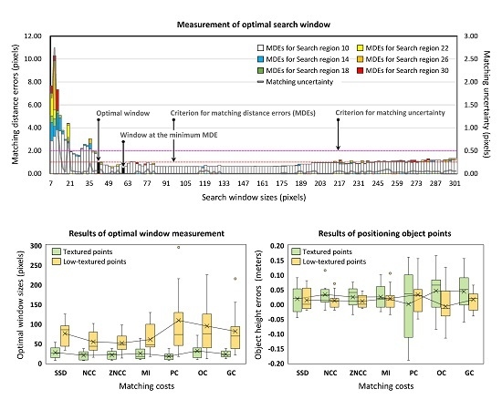
In this study, we define the optimal search window by the minimum window size that satisfies the two criteria of matching distance error and matching uncertainty. To decide the criteria for a given object point, matching distance errors are measured by applying different search window sizes and search region sizes (
Figure 2). Search window sizes are set from 7 × 7 pixels to 301 × 301 pixels, with 2-pixel intervals. Search region sizes are defined by increasing each search window by 10, 14, 18, 22, 26, and 30 pixels. For example, the search regions for the search window of 7 × 7 pixels are set to 17 × 17, 21 × 21, 25 × 25, 29 × 29, 33 × 33, and 37 × 37 pixels. In this study, a series of search regions, defined in this way, are named search region 10, 14, 18, 22, 26, and 30, respectively (
Figure 2). From these measurements, the optimal window is determined by the smallest search window, whose difference between the matching distance error and the minimum error is less than 0.5 pixels and matching uncertainty is less than 0.5 pixels. Note that this approach can only be applied to correct object points for the evaluation of matching costs.
2.5. Modeling Error
According to the principle of object space-based matching, matching costs should represent a decrease in matching distance errors as the height of the object point applied approaches the true value. Additionally, matching costs should produce the lowest error from the true height. However, even if the optimal search window is applied, matching distance errors can fluctuate as the height of the object point is adjusted (black line in
Figure 3). In this case, the heights of object points may be erroneously estimated due to the variation of matching distance errors. For this reason, we evaluate the uncertainty of matching costs in positioning object points by modeling the changes of matching distance errors and then by measuring the root mean square error (RMSE) between the actual and model values. In this model, the third-order polynomial and random sample consensus (RANSAC) algorithm is applied [
28]. This is used to consider the asymmetry and fluctuation of the matching distance errors around the true object height.
2.6. Convergence Angle
The reduction rate of the matching distance errors around the true height of the object point can also be an indicator for evaluating the uncertainty of matching costs. This is because the ambiguity in positioning object points can be largely minimized, as the matching distance errors are rapidly decreased. The reduction rate can be measured as the convergence angle, which is formed at the finally estimated height (
Figure 3b). The two points forming the convergence angle are assigned to the two locations, shifted by a ±1 ground sampling distance (GSD) from the finally estimated height. In this measurement, the modeled error values are used, instead of the measured errors, to correctly reflect the reduction tendency.
2.7. Height Error
The height error is proposed to evaluate the accuracy of matching costs, which is defined as the difference between the true object height and the estimated object height. In this study, we obtain the true heights of object points from a laser scanner dataset, because a Global Positioning System (GPS) survey is impossible on drifting sea-ice. More details of this procedure are described in
Section 3.2. On the other hand, the heights of object points are estimated by two-step modeling. First, an initial model is established for a predefined height adjustment range, and the initial height of the object point is estimated by measuring the minimum error in the initial model (
Figure 3a). Then, a precision model is established for a narrower height adjustment range, and the final height of the object point is determined from the precision model (
Figure 3b). The height adjustment range for the initial model is set from −0.3 m to 0.3 m around the height, with the minimum error measured. The height adjustment range for the precision model is set from −0.2 m to 0.2 m around the initially estimated object height. This approach is designed to better reflect the reduction tendency of matching distance errors.
2.8. Processing Time
The processing speed of matching costs is evaluated by measuring the time spent calculating the matching distance errors for different search window sizes. Search window sizes are set from 7 × 7 pixels to 301 × 301 pixels, with 2-pixel intervals. The search region size is set with a larger boundary of 5 pixels than that of the search windows. The processing time is separately measured for the image pre-processing, patch image generation, and matching distance error calculation steps on a platform, with CPU Intel Core i7-4790K, clock speed 4.0 GHz, and RAM 32 GB. For the reliability of the evaluation, the experiment is repeated 5 times, and the averages of the measurements are analyzed.
3. Materials
3.1. Aerial Image Dataset
In August 2017, the Korean icebreaker, Araon, conducted an Arctic sea-ice survey at 77.5879°N and 179.2901°E on the Chukchi Sea (
Figure 4a). During this survey, 25 drone images of sea-ice surfaces were obtained (
Figure 4b). The camera used for the image acquisition was an FC330, mounted on a DJI Phantom 4 (DJI, Shenzhen, China), with an image size of 4000 × 3000 pixels, a focal length of 3.6 mm, and a pixel size of 1.58 µm. The images were acquired over 3 min and 33 s, and the sea-ice moved linearly at a velocity of about 0.16 m/s during the acquisition time. The sea-ice drift was calculated from the GPS logger mounted on the Araon.
The internal and external camera parameters can be estimated through a bundle block adjustment from the tie-points between adjacent images and ground control points (GCPs). However, accurate georeferencing using GCPs was practically impossible, because sea-ice is constantly moving. For this reason, we estimated camera parameters, using only GPS and inertial navigation system (GPS/INS) data and tie-points, and then produced the mosaic image, with a GSD of 0.04 m. This work was conducted using the commercial software, Pix4D 4.1.24 (Pix4D SA, Lausanne, Switzerland). In general, the GPS information of the camera should be corrected to the drift of sea-ice prior to camera parameter estimation. This is because the drift of sea-ice may reduce not only the accuracy of georeferencing but also the accuracy of relative orientation in object space. In this study, however, we skipped the drift correction to the camera positions, because the movement of sea-ice was not large during the image acquisition. Although georeferencing accuracy may be reduced due to the sea-ice drift, we analyze the performance of matching costs using the registered scanner dataset. Therefore, the accuracy of georeferencing is not considered important in this study.
3.2. Analysis Points
From the sea-ice surface model, acquired by the laser scanner, FARO Focus3D X130, in the sea-ice survey, 3D object points were extracted. These are intended as accurate analysis points for the performance evaluation of matching costs. With a distance range of 0.6 to 130 m, a precision of 2 mm, a vertical rotation range of 300°, and a horizontal rotation range of 360°, the laser scanner collected point clouds and their intensities for the target area. Using these scanner datasets, we produced the mosaic image and the sea-ice surface model (
Figure 5b,c). In order to determine the heights of the analysis points, registration was conducted to align the coordinate system of the drone dataset with the coordinate system of the scanner dataset. In the registration process, 11 tie points, manually extracted between the drone mosaic and the scanner mosaic, were used (
Figure 5a,b). Registration errors were about 0.04, 0.03, and 0.04 m for X, Y, and Z axes, respectively. Since the GSD of the drone mosaic is about 0.04 m, the registration was considered to have been performed correctly.
Figure 5d shows the registered scanner sea-ice surface model. The gradient of surface elevation shown in
Figure 5d is likely to be due to the absence of ground control points. Since ground control points cannot be used in camera parameter estimation, the object space for the drone images has to be formed by only the tie-points between adjacent images and the GPS information of cameras. For this reason, if the reference coordinate system of object space is set by the camera tilted on the sea-ice surface, a gradient of surface elevation may occur. However, since this is not an error in relative orientation, it would not affect the analysis results in this study. On the other hand, the RMSE of the sea-ice surface model produced from the drone images was about 0.35 m, compared to the registered scanner sea-ice surface model. This result suggests that additional considerations are needed to create high-quality sea-ice surface models.
From the drone mosaic and the registered scanner sea-ice surface model, a total of 20 analysis points were extracted. Through visual inspection, the analysis points were divided into textured points (1st to 9th points) and low-textured points (10th to 20th points). These analysis points are considered ground truth data with true heights and are used to measure performance indicators.
Figure 6 shows the locations of the analysis points and several examples with different surface textures.
4. Results and Discussion
4.1. Robustness of Matching to Low-Textured Surfaces
The robustness of image matching to low-textured surfaces was evaluated using the optimal search windows, measured for the analysis points. The optimal window sizes showed a large increase in the low-textured points (
Table 1 and
Figure 7). In the textured points, the differences between matching costs were small, whereas in the low-textured points, the window sizes of the image domain costs were smaller than those of the frequency domain costs (
Figure 7b). Among the image domain costs, ZNCC showed the smallest window sizes, whereas SSD showed a relatively large increase in search window sizes due to the decrease in surface textures.
Meanwhile, the image domain costs showed lower matching distance errors, even with smaller search windows (
Table 2 and
Figure 8a), which was more pronounced in the results for the low-textured points (
Figure 8b). These improvements may be due to the fact that the elevation differences of sea-ice surfaces inside the search windows for the low-textured points were relatively smaller than those for the textured points. However, such improvements were not evident in the results for the frequency domain costs. These results, on the contrary, demonstrate the high discriminatory power of the image domain costs for low-textured surfaces.
Matching uncertainty due to change in surface textures was evaluated by dividing them into smaller search windows and larger search windows than the optimal search window. This is conducted with the aim of identifying the differences in matching uncertainty between a situation in which the search window sizes are properly applied and one in which they are not. In the case of insufficient search windows, matching costs generally represented high uncertainties for all analysis points (
Table 3;
Table 4). In particular, SSD, PC, and GC showed considerably high uncertainties (
Figure 9a). On the other hand, OC had significantly lower uncertainties than other matching costs. These results suggest that OC is more likely to find correct matches than other matching costs when it is difficult to apply appropriate search windows, which explains the high matching success rate of OC in the existing cryospheric studies, in which a search window of a fixed size is applied [
26,
29,
30].
Figure 10 illustrates an example of matching distance errors measured from different search windows and search regions. In the case of OC, we can see that the variation of matching distance errors is very low in search windows that are smaller than the optimal search window, as compared to other matching costs.
On the other hand, the matching uncertainties of all the matching costs were significantly reduced when sufficiently sized search windows were applied. In particular, NCC, ZNCC, and MI showed fairly low matching uncertainties (
Figure 9b). These results suggest that the search window size should be adjusted variably on low-textured surfaces, such as sea-ice. In this case, image domain costs showed more reliable and accurate matching results than those of frequency domain costs, even with smaller search windows. Therefore, we could conclude that NCC, ZNCC, and MI are more effective in terms of template matching, assuming that optimal windows can be applied.
4.2. Robustness of Positioning to Low-Textured Surfaces
The robustness of positioning to low-textured surfaces was evaluated by measuring the modeling error, convergence angle, and height error, where these indicators were calculated by applying the optimal search windows for each analysis point. In positioning object points, the modeling errors and convergence angles indicate the uncertainty of positioning, and the height errors indicate the accuracy of positioning.
The modeling errors were relatively lower in the image domain costs (
Table 5 and
Figure 11a). Unlike the image domain costs, the frequency domain costs exhibited high modeling error distributions between the analysis points and, in particular, a sharp increase in modeling errors at the low-textured points (
Figure 11b). Convergence angles were also lower in the image domain costs (
Table 6 and
Figure 12a). Among the results for the frequency domain costs, only those of OC were similar to those of the image domain costs. Meanwhile, unlike the modeling errors, all the matching costs represented a decrease in convergence angles at the low-textured points (
Figure 12b).
In response to the results for modeling errors and convergence angles, the height errors were also relatively smaller in the image domain costs (
Table 7 and
Figure 13). In addition, the height errors of the image domain costs decreased at the low-textured points. This was probably due to the decrease in elevation differences within search windows, as explained earlier. Among the image domain costs, ZNCC showed the best performance. On the other hand, the frequency domain costs were similar to the image domain costs, in terms of mean error, but showed large variations in terms of error distribution. The OC produced similar convergence angles to the image domain costs but caused an increase in height errors due to large modeling errors. The GC did not produce large modeling errors but caused an increase in height errors due to large convergence angles. The PC, with the largest modeling errors and convergence angles, showed the greatest reduction in positioning accuracy. These results suggest that various parameters, such as modeling error and convergence angle, may affect the positioning of object points, even if sufficient textures have been considered in image matching. However, even in this situation, the image domain costs produced relatively reliable and accurate results. Therefore, assuming that the optimal search windows can be applied, all of the image domain costs could be effectively used in positioning object points on low-textured surfaces.
In this study, however, the robustness for radiometric differences was not addressed, because the drone images were acquired in a short time (i.e., 3 min and 33 s). Therefore, it should be noted that SSD and NCC, which are sensitive to radiometric differences, may cause performance degradation if images with different acquisition times are used.
As an additional experiment, the proposed method for positioning object points was verified. The evaluation was made by comparing the proposed method with the measurement method, which determines the height of an object point from the minimum value of the measured matching distance errors. In the experimental results, the proposed method showed a better performance (
Table 8 and
Figure 14). This is because the proposed method could reduce the uncertainty due to the variation of matching distance errors by considering the overall tendency around the true heights. In addition, since this method has continuity, the heights of object points can be determined with a higher precision. These results demonstrate the effectiveness of the proposed method in positioning object points.
4.3. Evaluation of Processing Time
In this study, 3 × 3 median filtering was performed on original drone images, as basic image preprocessing. This was conducted with the aim of reducing image noise, while minimizing the loss of sharpness. In the case of OC and GC, the generation of orientation images and gradient images was added to the preprocessing step. For this reason, in preprocessing time, SSD, NCC, ZNCC, MI and PC were the same, while OC and GC were considerably longer (
Table 9). In patch image generation time, the matching costs, except for OC and GC, were also the same, whereas OC and GC were about twice as long, because they handle complex data. In terms of matching the distance error calculation time, PC was the shortest. This is because the image matching in the frequency domain can be made by only one matrix multiplication. This Fourier shift theorem is also commonly applied in OC and GC, but they required more time to deal with both real and imaginary parts. As a result, SSD, NCC and ZNCC, rather than OC and GC, consumed less processing time in calculating matching distance errors. However, if the application purpose is template matching for a wide search area, OC and GC would have a better performance in terms of processing speed than the image domain costs. On the other hand, MI spent a lot of time measuring matching distance errors, because it involves many computations in entropy calculation. Consequently, in terms of the total processing time, PC showed the best performance, but SSD, NCC and ZNCC were not far behind.
5. Conclusions
We evaluated the performance of the matching costs used in various applications. In order to examine considerations pertaining to the creation of high-quality sea-ice surface models, the evaluation focused on the robustness of matching and positioning to low-textured surfaces and the processing speed. From the evaluation results, we found that the image domain costs were more effective for low-textured surfaces of sea-ice than the frequency domain costs. In terms of matching robustness, the image domain costs, except SSD, showed a better performance, even with smaller search windows. Exceptionally, however, OC, one of the frequency domain costs, is expected to be more effective when a fixed search window size is applied. In terms of positioning robustness, the image domain costs also performed better because of the lower modeling errors and narrower convergence angles. Lastly, in terms of processing speed, the PC of the frequency domain showed the best performance, but SSD, NCC, and ZNCC were not far behind. From these evaluation results, we concluded that, among the matching costs, ZNCC would be the most effective for sea-ice surface model generation. ZNCC showed a high accuracy and stability, both in terms of matching and positioning, even with the smallest search windows, as well as a good performance in terms of processing speed.
The evaluation results suggest that appropriate search windows, in terms of the texture amounts, should be applied to find matching points on low-textured surfaces and that several uncertainties due to low-textured surfaces should be considered to determine the positions of object points. These considerations indicate that optimal search window derivation and robust object positioning are essential for producing high-quality sea-ice surface models. Therefore, in a future study, we will develop a novel matching method that accommodates these considerations. We believe that the proposed performance indicators and the findings can contribute to various applications in cryosphere sciences through the development of optimized image-matching methods.
Author Contributions
Conceptualization, J.-I.K.; Formal analysis, J.-I.K., C.-U.H., H.H. and H.-c.K.; Methodology, J.-I.K.; Supervision, H.-c.K.; Writing–original draft, J.-I.K., C.-U.H., H.H. and H.-c.K.; Writing–review and editing, J.-I.K., C.-U.H., H.H. and H.-c.K.
Funding
This research was funded by the Korea Polar Research Institute (KOPRI), grant PE19120 (Research on analytical technique for satellite observation of Arctic sea ice).
Conflicts of Interest
The authors declare no conflict of interest.
References
- Vihma, T. Effect of Arctic sea-ice decline on weather and climate: A review. Surv. Geophys. 2014, 35, 1175–1214. [Google Scholar] [CrossRef]
- Aksenov, Y.; Popova, E.E.; Yool, A.; Nurser, A.J.G.; Williams, T.D.; Bertino, L.; Bergh, J. On the future navigability of Arctic sea routes: High-resolution projections of the Arctic Ocean and sea-ice. Mar. Policy 2017, 75, 300–317. [Google Scholar] [CrossRef]
- Nolin, A.W.; Mar, E. Arctic sea ice surface roughness estimated from multi-angular reflectance satellite imagery. Remote Sens. 2019, 11, 50. [Google Scholar] [CrossRef]
- Kim, H.; Han, H.; Hyun, C.; Chi, J.; Son, Y.; Lee, S. Research on analytical technique for satellite observation of the Arctic sea ice. Korea J. Remote Sens. 2019, 34, 1283–1298. [Google Scholar]
- Karvonen, J.; Cheng, B.; Vihma, T.; Arkett, M.; Carrieres, T. A method for sea-ice thickness and concentration analysis based on SAR data and a thermodynamic model. Cryosphere 2012, 6, 1507–1526. [Google Scholar] [CrossRef]
- Wang, X.; Key, J.R. Arctic Surface, Cloud, and Radiation Properties Based on the AVHRR Polar Pathfinder Dataset. Part I: Spatial and Temporal Characteristics. J. Clim. 2005, 18, 2558–2574. [Google Scholar] [CrossRef]
- Hong, S.-H.; Wdowinski, S.; Amelung, F.; Kim, H.-C.; Won, J.-S.; Kim, S.-W. Using TanDEM-X Pursuit Monostatic Observations with a Large Perpendicular Baseline to Extract Glacial Topography. Remote Sens. 2018, 10, 1851. [Google Scholar] [CrossRef]
- Tschudi, M.A.; Maslanik, J.A.; Perovich, D.K. Derivation of melt pond coverage on Arctic sea-ice using MODIS observations. Remote Sens. Environ. 2008, 112, 2605–2614. [Google Scholar] [CrossRef]
- Hagen, R.; Peters, M.; Liang, R.; Ball, D.; Brozena, J. Measuring Arctic sea-ice motion in real time with photogrammetry. IEEE Geosci. Remote Sens. Lett. 2014, 11, 1956–1960. [Google Scholar] [CrossRef]
- Divine, D.V.; Pedersen, C.A.; Karlsen, T.I.; Aas, H.F.; Granskog, M.A.; Hudson, S.R.; Gerland, S. Photogrammetric retrieval and analysis of small scale sea-ice topography during summer melt. Cold Reg. Sci. Technol. 2016, 129, 77–84. [Google Scholar] [CrossRef]
- Veksler, O. Fast variable window for stereo correspondence using integral images. In Proceedings of the IEEE Conference on Computer Vision and Pattern Recognition, Madison, WI, USA, 18–20 June 2003; Volume 1, pp. 556–561. [Google Scholar]
- Brown, L. A survey of image registration techniques. ACM Comput. Surv. 1992, 24, 325–376. [Google Scholar] [CrossRef]
- Wang, L.; Zhang, Y.; Feng, J. On the Euclidean distance of images. IEEE Trans. Pattern Anal. Mach. Intell. 2005, 27, 1334–1339. [Google Scholar] [CrossRef] [PubMed]
- Nakhmani, A.; Tannenbaum, A. A new distance measure based on generalized Image Normalized Cross-Correlation for robust video tracking and image recognition. Pattern Recognit. Lett. 2013, 34, 315–321. [Google Scholar] [CrossRef]
- Hirschmuller, H.; Scharstein, D. Evaluation of cost functions for stereo matching. In Proceedings of the IEEE Conference on Computer Vision and Pattern Recognition, Minneapolis, MN, USA, 17–22 June 2007; pp. 1–8. [Google Scholar]
- Banks, J.; Bennamoun, M.; Corke, P. Fast and robust stereo matching algorithms for mining automation. Digit. Signal Process. 1999, 9, 137–148. [Google Scholar] [CrossRef]
- Banks, J.; Corke, P. Quantitative evaluation of matching methods and validity measures for stereo vision. Int. J. Robot. Res. 2001, 20, 512–532. [Google Scholar] [CrossRef]
- Hirschmuller, H.; Scharstein, D. Evaluation of stereo matching costs on images with radiometric differences. IEEE Trans. Pattern Anal. Mach. Intell. 2009, 31, 1582–1599. [Google Scholar] [CrossRef]
- Kim, J.; Kim, H. Performance comparison of matching cost functions for high-quality sea-ice surface model generation. Korean J. Remote Sens. 2018, 34, 1251–1260. [Google Scholar]
- Zhang, K.; Sheng, Y.; Wang, M.; Fu, S. An enhanced multi-view vertical line locus matching algorithm of object space ground primitives based on positioning consistency for aerial and space images. ISPRS J. Photogramm. Remote Sens. 2018, 139, 241–254. [Google Scholar] [CrossRef]
- Zhang, Y.; Zhang, Y.; Mo, D.; Zhang, Y.; Li, X. Direct digital surface model generation by semi-global vertical line locus matching. Remote Sens. 2017, 9, 214. [Google Scholar] [CrossRef]
- Elboher, E.; Werman, M. Asymmetric correlation: A noise robust similarity measure for template matching. IEEE Trans. Image Process. 2013, 22, 3062–3073. [Google Scholar] [CrossRef]
- Pluim, J.P.W.; Maintz, J.B.A.; Viergever, M.A. Mutual-information-based registration of medical images: A survey. IEEE Trans. Med. Imaging 2003, 22, 986–1004. [Google Scholar] [CrossRef]
- Reddy, B.S.; Chatterji, B.N. An FFT-based technique for translation, rotation, and scale-invariant image registration. IEEE Trans. Image Process. 1996, 5, 1266–1271. [Google Scholar] [CrossRef]
- Fitch, A.J.; Kadyrov, A.; Christmas, W.J.; Kittler, J. Orientation correlation. In Proceedings of the British Machine Vision Conference, Cardiff, UK, 2–5 September 2002; pp. 133–142. [Google Scholar]
- Heid, T.; Kääb, A. Evaluation of existing image matching methods for deriving glacier surface displacements globally from optical satellite imagery. Remote Sens. Environ. 2012, 118, 339–355. [Google Scholar] [CrossRef]
- Argyriou, V.; Vlachos, T. Estimation of sub-pixel motion using gradient cross-correlation. Electron. Lett. 2003, 39, 980–982. [Google Scholar] [CrossRef]
- Fischler, M.A.; Bolles, R.C. Random sample consensus: A paradigm for model fitting with applications to image analysis and automated cartography. Commun. ACM 1981, 24, 381–395. [Google Scholar] [CrossRef]
- Han, H.; Im, J.; Kim, H. Variations in ice velocities of Pine Island Glacier Ice Shelf evaluated using multispectral image matching of Landsat time series data. Remote Sens. Environ. 2016, 186, 358–371. [Google Scholar] [CrossRef]
- Han, H.; Lee, C.-K. Analysis of ice variations of Nansen Ice Shelf, East Antarctica from 2000 to 2017 using Landsat multispectral image matching. Korean J. Remote Sens. 2018, 34, 1165–1178. [Google Scholar]
Figure 1.
Definition of the matching distance error.
Figure 1.
Definition of the matching distance error.
Figure 2.
An example of an optimal window measurement.
Figure 2.
An example of an optimal window measurement.
Figure 3.
Model of the matching distance errors, measured at each height. (a) Initial model for the wide height adjustment range; and (b) precision model for the narrow height adjustment range, centered on the initially determined object height.
Figure 3.
Model of the matching distance errors, measured at each height. (a) Initial model for the wide height adjustment range; and (b) precision model for the narrow height adjustment range, centered on the initially determined object height.
Figure 4.
(a) Location of the sea-ice survey; and (b) overview of the drone image acquisition on the sea-ice surfaces.
Figure 4.
(a) Location of the sea-ice survey; and (b) overview of the drone image acquisition on the sea-ice surfaces.
Figure 5.
Registration between the drone and scanner datasets. (
a) Drone mosaic, (
b) scanner mosaic, (
c) scanner sea-ice surface model, generated from the scanner point cloud data [
19], and (
d) registered scanner sea-ice surface model.
Figure 5.
Registration between the drone and scanner datasets. (
a) Drone mosaic, (
b) scanner mosaic, (
c) scanner sea-ice surface model, generated from the scanner point cloud data [
19], and (
d) registered scanner sea-ice surface model.
Figure 6.
Locations of the analysis points and several examples with different surface textures. This figure was formulated by editing
Figure 5;
Figure 6 from the work of Kim and Kim [
19].
Figure 6.
Locations of the analysis points and several examples with different surface textures. This figure was formulated by editing
Figure 5;
Figure 6 from the work of Kim and Kim [
19].
Figure 7.
Statistical distributions of the optimal window sizes for the sum of squared differences (SSD), normalized cross-correlation (NCC), zero-mean NCC (ZNCC), mutual information (MI), phase correlation (PC), orientation correlation (OC) and gradient correlation (GC). (a) Window size distribution for all analysis points, and (b) window size distributions for each of the textured and low-textured points.
Figure 8.
Statistical distributions of the matching distance errors. (a) Error distribution for all analysis points, and (b) error distributions for each of the textured and low-textured points.
Figure 8.
Statistical distributions of the matching distance errors. (a) Error distribution for all analysis points, and (b) error distributions for each of the textured and low-textured points.
Figure 9.
Statistical distributions of matching uncertainties: (a) Matching uncertainties for insufficient window sizes, and (b) matching uncertainties for appropriate window sizes.
Figure 9.
Statistical distributions of matching uncertainties: (a) Matching uncertainties for insufficient window sizes, and (b) matching uncertainties for appropriate window sizes.
Figure 10.
Matching distance errors measured from different search windows and search regions for the 7th analysis point. (a) SSD, (b) NCC, (c) ZNCC, (d) MI, (e) PC, (f) OC, and (g) GC.
Figure 10.
Matching distance errors measured from different search windows and search regions for the 7th analysis point. (a) SSD, (b) NCC, (c) ZNCC, (d) MI, (e) PC, (f) OC, and (g) GC.
Figure 11.
Statistical distributions of the modelling errors. (a) Error distributions for all the analysis points, and (b) error distributions for each of the textured and low-textured points.
Figure 11.
Statistical distributions of the modelling errors. (a) Error distributions for all the analysis points, and (b) error distributions for each of the textured and low-textured points.
Figure 12.
Statistical distributions of the convergence angles. (a) Convergence angle distributions for all the analysis points, and (b) convergence angle distributions for each of the textured and low-textured points.
Figure 12.
Statistical distributions of the convergence angles. (a) Convergence angle distributions for all the analysis points, and (b) convergence angle distributions for each of the textured and low-textured points.
Figure 13.
Statistical distributions of the height errors. (a) Error distribution for all analysis points and (b) error distributions for the textured and low-textured points.
Figure 13.
Statistical distributions of the height errors. (a) Error distribution for all analysis points and (b) error distributions for the textured and low-textured points.
Figure 14.
Comparison of height error distributions using the measuring approach and the modelling approach.
Figure 14.
Comparison of height error distributions using the measuring approach and the modelling approach.
Table 1.
Optimal window sizes of the sum of squared differences (SSD), normalized cross-correlation (NCC), zero-mean NCC (ZNCC), mutual information (MI), phase correlation (PC), orientation correlation (OC) and gradient correlation (GC) measured for the analysis points (unit: pixels).
Table 1.
Optimal window sizes of the sum of squared differences (SSD), normalized cross-correlation (NCC), zero-mean NCC (ZNCC), mutual information (MI), phase correlation (PC), orientation correlation (OC) and gradient correlation (GC) measured for the analysis points (unit: pixels).
| Points | SSD | NCC | ZNCC | MI | PC | OC | GC |
|---|
| All | 54 ± 34 | 39 ± 28 | 37 ± 25 | 44 ± 34 | 68 ± 75 | 66 ± 57 | 55 ± 50 |
| Textured | 27 ± 14 | 20 ± 11 | 21 ± 10 | 25 ± 17 | 17 ± 9 | 31 ± 18 | 23 ± 9 |
| Low-Textured | 76 ± 30 | 54 ± 28 | 51 ± 25 | 60 ± 35 | 109 ± 79 | 94 ± 63 | 81 ± 54 |
Table 2.
Matching distance errors measured at the optimal window sizes (unit: pixels).
Table 2.
Matching distance errors measured at the optimal window sizes (unit: pixels).
| Points | SSD | NCC | ZNCC | MI | PC | OC | GC |
|---|
| All | 1.2 ± 0.4 | 1.2 ± 0.3 | 1.2 ± 0.3 | 1.2 ± 0.4 | 1.4 ± 0.3 | 1.4 ± 0.3 | 1.4 ± 0.3 |
| Textured | 1.4 ± 0.3 | 1.3 ± 0.3 | 1.4 ± 0.3 | 1.3 ± 0.4 | 1.5 ± 0.2 | 1.4 ± 0.4 | 1.4 ± 0.3 |
| Low-Textured | 1.0 ± 0.3 | 1.0 ± 0.2 | 1.0 ± 0.2 | 1.1 ± 0.2 | 1.3 ± 0.4 | 1.4 ± 0.2 | 1.3 ± 0.2 |
Table 3.
Matching uncertainty with insufficient window sizes (unit: pixels).
Table 3.
Matching uncertainty with insufficient window sizes (unit: pixels).
| Points | SSD | NCC | ZNCC | MI | PC | OC | GC |
|---|
| All | 1.49 ± 0.83 | 0.74 ± 0.56 | 0.87 ± 0.58 | 1.00 ± 0.53 | 1.15 ± 1.33 | 0.45 ± 0.31 | 0.88 ± 1.12 |
| Textured | 1.51 ± 0.97 | 0.50 ± 0.48 | 0.62 ± 0.49 | 0.92 ± 0.58 | 1.81 ± 1.74 | 0.54 ± 0.43 | 1.25 ± 1.53 |
| Low-Textured | 1.48 ± 0.69 | 0.93 ± 0.55 | 1.08 ± 0.57 | 1.06 ± 0.48 | 0.61 ± 0.33 | 0.38 ± 0.12 | 0.58 ± 0.41 |
Table 4.
Matching uncertainty with appropriate window sizes (unit: pixels).
Table 4.
Matching uncertainty with appropriate window sizes (unit: pixels).
| Points | SSD | NCC | ZNCC | MI | PC | OC | GC |
|---|
| All | 0.08 ± 0.11 | 0.05 ± 0.05 | 0.05 ± 0.06 | 0.04 ± 0.04 | 0.11 ± 0.06 | 0.09 ± 0.03 | 0.09 ± 0.02 |
| Textured | 0.06 ± 0.10 | 0.05 ± 0.07 | 0.05 ± 0.08 | 0.05 ± 0.06 | 0.10 ± 0.03 | 0.10 ± 0.03 | 0.10 ± 0.03 |
| Low-Textured | 0.10 ± 0.11 | 0.05 ± 0.01 | 0.05 ± 0.02 | 0.03 ± 0.01 | 0.12 ± 0.07 | 0.09 ± 0.02 | 0.08 ± 0.01 |
Table 5.
Modelling errors for the analysis points (unit: pixels).
Table 5.
Modelling errors for the analysis points (unit: pixels).
| Points | SSD | NCC | ZNCC | MI | PC | OC | GC |
|---|
| All | 0.17 ± 0.04 | 0.16 ± 0.05 | 0.15 ± 0.04 | 0.16 ± 0.04 | 0.22 ± 0.12 | 0.20 ± 0.07 | 0.16 ± 0.11 |
| Textured | 0.17 ± 0.04 | 0.15 ± 0.04 | 0.13 ± 0.04 | 0.18 ± 0.06 | 0.17 ± 0.12 | 0.16 ± 0.06 | 0.16 ± 0.15 |
| Low-Textured | 0.17 ± 0.04 | 0.17 ± 0.05 | 0.16 ± 0.03 | 0.16 ± 0.03 | 0.26 ± 0.11 | 0.23 ± 0.06 | 0.16 ± 0.06 |
Table 6.
Convergence angles for the analysis points (unit: degrees).
Table 6.
Convergence angles for the analysis points (unit: degrees).
| Points | SSD | NCC | ZNCC | MI | PC | OC | GC |
|---|
| All | 52 ± 16 | 54 ± 15 | 54 ± 13 | 51 ± 10 | 74 ± 32 | 55 ± 14 | 65 ± 32 |
| Textured | 65 ± 15 | 63 ± 17 | 63 ± 15 | 56 ± 12 | 98 ± 29 | 60 ± 19 | 81 ± 40 |
| Low-Textured | 42 ± 5 | 46 ± 6 | 46 ± 4 | 48 ± 5 | 54 ± 17 | 51 ± 6 | 53 ± 13 |
Table 7.
Height errors estimated for the analysis points (unit: meters).
Table 7.
Height errors estimated for the analysis points (unit: meters).
| Points | SSD | NCC | ZNCC | MI | PC | OC | GC |
|---|
| All | 0.02 ± 0.04 | 0.02 ± 0.03 | 0.02 ± 0.03 | 0.02 ± 0.04 | 0.02 ± 0.09 | 0.02 ± 0.07 | 0.03 ± 0.05 |
| Textured | 0.02 ± 0.04 | 0.03 ± 0.04 | 0.02 ± 0.03 | 0.03 ± 0.04 | 0.00 ± 0.11 | 0.05 ± 0.07 | 0.04 ± 0.06 |
| Low-Textured | 0.01 ± 0.03 | 0.01 ± 0.03 | 0.01 ± 0.02 | 0.02 ± 0.04 | 0.03 ± 0.06 | −0.01 ± 0.06 | 0.02 ± 0.03 |
Table 8.
Height errors of the measuring approach to object height estimation (unit: meters).
Table 8.
Height errors of the measuring approach to object height estimation (unit: meters).
| Points | SSD | NCC | ZNCC | MI | PC | OC | GC |
|---|
| All | 0.02 ± 0.04 | 0.02 ± 0.06 | 0.02 ± 0.04 | 0.03 ± 0.06 | 0.03 ± 0.10 | 0.01 ± 0.06 | 0.02 ± 0.07 |
| Textured | 0.03 ± 0.04 | 0.03 ± 0.07 | 0.04 ± 0.04 | 0.03 ± 0.06 | 0.06 ± 0.13 | 0.05 ± 0.05 | 0.03 ± 0.09 |
| Low-Textured | 0.01 ± 0.04 | 0.01 ± 0.04 | 0.01 ± 0.04 | 0.02 ± 0.06 | 0.00 ± 0.04 | −0.02 ± 0.05 | 0.02 ± 0.03 |
Table 9.
Processing time of the matching costs (unit: seconds).
Table 9.
Processing time of the matching costs (unit: seconds).
| | SSD | NCC | ZNCC | MI | PC | OC | GC |
|---|
| Pre-Processing | 0.13 | 0.13 | 0.13 | 0.13 | 0.13 | 13.31 | 3.78 |
| Patch Extraction | 5.74 | 5.69 | 5.72 | 5.80 | 5.75 | 10.57 | 10.66 |
| MDE Measurement | 15.62 | 15.72 | 15.74 | 325.80 | 14.74 | 17.59 | 17.61 |
| Total Time | 21.50 | 21.54 | 21.60 | 331.74 | 20.63 | 41.48 | 32.06 |
© 2019 by the authors. Licensee MDPI, Basel, Switzerland. This article is an open access article distributed under the terms and conditions of the Creative Commons Attribution (CC BY) license (http://creativecommons.org/licenses/by/4.0/).


