Energy Efficient and Delay Aware 5G Multi-Tier Network

Abstract

Multi-tier heterogeneous Networks (HetNets) with dense deployment of small cells in 5G networks are expected to effectively meet the ever increasing data traffic demands and offer improved coverage in indoor environments. However, HetNets are raising major concerns to mobile network operators such as complex distributed control plane management, handover management issue, increases latency and increased energy expenditures. Sleep mode implementation in multi-tier 5G networks has proven to be a very good approach for reducing energy expenditures. In this paper, a Markov Decision Process (MDP)-based algorithm is proposed to switch between three different power consumption modes of a base station (BS) for improving the energy efficiency and reducing latency in 5G networks. The MDP-based approach intelligently switches between the states of the BS based on the offered traffic while maintaining a prescribed minimum channel rate per user. Simulation results show that the proposed MDP algorithm together with the three-state BSs results in a significant gain in terms of energy efficiency and latency.

1. Introduction

The next generation (5G) of wireless networks will serve an unprecedented number of devices, providing ubiquitous connectivity as well as innovative and rate-demanding services. Hence the design of 5G networks will necessarily have to consider energy efficiency as one of its key pillars. Recent studies prove that using a multi-tier 5G network is a very good approach to reduce energy consumption in the entire network [1]. Furthermore, the gain might be very high if the architecture allows switching off the network resources or base stations (BSs) that are not necessary to guarantee the target QoS for the offered traffic. In that case, minimal or zero power consumption mode of a base station can play a very crucial role if the aim is to increase energy efficiency of the network. Thus a 5G BS, which is known as gNB, can be turned off or put in low power consumption mode to reduce global energy consumption when its service not needed to ensure QoS. However we should also consider the delay caused by the required wake up time from sleep mode. The deepest sleep mode consumes zero power, however can cause significant delay in service due to wake up time from sleep mode; whereas in a lighter sleep mode (also known as stand-by mode) a resource consumes little power but wakes up very quickly. Hence our proposed model fills a gap in the performance evaluation of two type of minimal power consumption mode with a trade–off between energy efficiency and wake-up delay, while ensuring user-perceived QoS. In this work, low and zero power consumption modes are implemented on the BSs of a multi-tier 5G network in order to reduce the energy consumption of the network. We propose three different power consumption modes for BSs and a novel MDP-based algorithm to control these modes of the BSs under QoS constraint.

Novelty of our work: As already presented in some pioneering works [2,3,4], switching off a base station within a HetNet is a very good approach to save energy consumption during low traffic condition. However each sleeping BS takes significant amount of time to wake up and become fully operable. As a consequence, some of the users might experience a delay in accessing the network, even some calls might be dropped as well. In order to overcome the problem of call dropping due to the wake up delay, we propose an energy efficient ‘3-state MDP model’ for the BSs within the network. We propose three different modes namely ‘Active mode’, ‘Stand-by mode’ and ‘Sleep mode’ for the BSs. In this paper, we utilize Markov model to find the optimal policy in terms of energy efficiency using Markov decision process (MDP). We have also shown the energy-delay trade–off in order to design an energy efficient as well as delay aware network. We utilize the stand-by mode and have differentiated it from the sleep mode by defining that a BS in stand-by mode consumes some small amount of energy but takes negligible time to go back to the active mode; whereas a BS in sleep mode does not consume any energy but takes more time to wake up. Hence sleep mode gives us the advantage of power saving, whereas stand-by mode allows us to avoid the wake-up delay. That is why we are implementing both the stand-by mode and sleep mode in our algorithm so that we can reduce energy consumption as well as wake up delay of BSs. The hardware and software setups for these low power consumption and zero power consumption modes have already been proposed in the literature [5,6]. We have explained the operation and switching procedure among these modes in the following sections. Another novelty of our work is in defining a novel reward function for the Markov decision process (MDP) which helps us to get an optimal policy in selecting a particular mode for each BS. Because of applying the proposed 3-state MDP model, we find that a significant amount of energy can be saved in low traffic condition along with fulfilling the QoS requirement in terms of data rate.

The rest of the paper is organized as follows: Section 2 outlines related work in the concerned area. Network model, three state Markov model and proposed MDP-based algorithm model are presented in Section 3, Section 4 and Section 5, respectively. Section 6 presents the power consumption model. The simulation results and performance analysis are presented in Section 7. Finally Section 8 concludes the paper.

2. Related Work

Energy efficiency in cellular networks and communication has been studied widely in the literature [2,3,4,5,7,8,9]. Some research papers [2,3,4,5] have proposed different algorithms to implement sleep mode in the LTE BSs. The authors in [5] proposed an approach to reduce energy consumption in mobile networks by introducing discontinuous transmission on the base station side. In some of the pioneering works, MDP has been used as an effective approach for sleep mode implementation [2,7,8,9] for green communication as well as to solve some other optimization problems [10,11]. The authors in [10] use a Markov decision process-based model to schedule consumers’ behaviors in order to optimize the consumers’ net benefits. They utilize a networked smart grid system, where future electricity generation is predicted with reasonable accuracy based on weather forecasts. In [11], the authors have proposed an algorithm to design efficient coding tools and optimize frame structure for transmission to facilitate view switching and contain error propagation in differentially coded video due to packet losses. In [2], the authors proposed an MDP-based optimal controller that associates to an activation/deactivation policy which maximizes a multiple objective function of the QoS and improve energy efficiency. Other papers such as [7,8] consider a single user and use a Markov chain technique to evaluate the energy savings due to the sleep mode mechanism of a single user terminal. The authors in [8] take correlated packet arrivals into account to evaluate an MDP-based sleep mode mechanism. The authors in [9] consider a similar setting of one user and one station and show how to derive the optimal sleep policy numerically by formalizing the problem as a Semi-MDP. The authors in [3] proposed a novel scheme for the sleep scheduling based on decentralized partially observable MDP (Dec-POMDP). However almost all of the above mentioned papers have proposed sleep mode of the BS in low traffic condition and the BS will be in active mode for rest of the time. We refer to this model as ‘2-state model’. The authors of references [2,3,4,5,12] have shown that this 2-state power consumption model can reduce energy consumption of the whole network. However, the problem is that the BS takes significant time to wake up from sleep mode, which may cause call drop to new users. This wake up time can range from tens of seconds to couple of minutes for small cell and up to 10–15 min for macro cell [6]. This is clearly a constraint for an energy efficient system. The authors in reference [5] proposed the low power consumption mode, which consumes some small amount of power but wakes up within negligible time; their power consumption model is similar to what we propose as stand-by mode. In contrast to works done in the literature so far, we propose a MDP-based algorithm on the base stations so that they can intelligently switch among three different modes.

3. Network Model

We consider a multi-tier 5G network where some base stations can be put in low power consumption mode as shown in Figure 1. In our proposed model we are implementing low and zero power consumption mode on the base stations within this multi-tier 5G network. The proposed algorithm is managed in the algorithm management unit, which is included in the base band unit of the network architecture. The Mobility Management Entity (MME) unit of the Evolved Packet Core (EPC) also has some contribution in the algorithm, as MME can inform the BS if any new user is approaching the cell and if any handover is about to happen. Thus, the MME can help the BS to update the total number of active users. Hence the centralized management unit is included in the mobility management entity (MME). The home subscriber server (HSS), mobility management entity (MME), serving gateway (S-GW) and packet data network gateway (P-GW) are included in the evolved packet core (EPC). The nomenclature used in rest of the paper is provided in

Table 1. The acronyms and terms.

Acronyms	Description
BS	Base Station
MDP	Markov decision model
QOS	Quality of service
$B{W}_T$	Total bandwidth offered by BS
$N_{act}$	Number of active BS
$N_{std}$	Number of stand-by BS
$N_{slp}$	Number of BS in sleep mode
N	Total number of BSs in the network
${\mathsf{\P }}_{out}$	Transmit power
${\mathsf{\P }}_{act}$	Power consumption in active mode
${\mathsf{\P }}_{std}$	Power consumption in stand-by mode
${\mathsf{\P }}_{slp}$	Power consumption in sleep mode

.

Traffic Model: We adopt a traffic model where the users arrive according to Poisson process in the coverage area of the BS with a certain arrival rate, $u_{\lambda }$ and death rate, $u_{\mu }$. Here we include all the users originating calls in the cell as well as the users being handed over from other cells.

Propagation Channel Model: We consider the log-normal shadowing model with a pathloss exponent, $\alpha$ and a shadowing variance, $\sigma$ under AWGN channel. The received signal to noise ratio (SNR) per user is determined by link budget calculation from Equation (1), where ${\mathsf{\P }}_{out}$ is the transmit power of the BS; $PL$ is pathloss; $G_t$ and $G_r$ are transmit and received antenna gain respectively; X is log-normal shadowing and $P_n$ is the noise power. Equation (2) is used to find the pathloss $PL$, where $d_0$ is a reference distance, $f_c$ is carrier frequency, c is the speed of light and d is the distance between the BS and the user. Please note that for the sake of simplicity, we consider zero level of interference in the network. The values of $d_0$ and c are constant and are provided in

Table 2. BS’s parameters for the power consumption model.

Parameters	Values
Carrier frequency, $f_c$	1800 MHz
Path Loss Exponent, $\alpha$	2.5
BS Transmit Power	40 W
Shadowing Mean	0
Variance, $\sigma$	7
Total BSs, N	3
Antenna Gain	10 dB and 2 dB
User arrival rate, $\lambda$	0.01
User death rate, $\mu$	0.005
${\mathsf{\P }}_{max}$	40 W
Minimum data rate	300 kbps
$d\mathsf{\P }$	$4.7$
${\mathsf{\P }}_{std}$	10 W
${\mathsf{\P }}_{slp}$	0 W
$B{W}_T$	6 MHz
$b_{max}$	6 MHz
$b_{min}$	2 MHz
BW per BS	2 MHz
$dt$	2 s
$d_0$	1 km
c	$3\times {10}^8$ ms${}^{-1}$

.

$$SNR\left(dB\right)={\mathsf{\P }}_{out}+G_t+G_r-PL-X-P_n$$

(1)

$$PL=20log(\frac{4\pi d_0{f}_c}{c})+10\alpha log(\frac{d}{d_0})$$

(2)

Then Shannon’s capacity formula [13] is used to determine the required bandwidth for all of the active users for a minimum target data rate, as shown in Equation (3); here $R_t$ is the target data rate and $snr$ is signal to noise ratio in linear value. This $B{W}_{req}$ is the measure of the minimum required QoS. Our proposed algorithm ensures that this QoS requirement is fulfilled while reducing energy consumption and delay.

$$B{W}_{req}=\frac{R_t}{lo{g}_2(1+snr)}$$

(3)

4. Proposed Power Consumption Modes

We have proposed a three state model, where the BSs of the network can be in any of the following three states:

• Active Mode: In active mode, the BS is in fully operational mode and consumes maximum power.
• Stand-by Mode: In stand-by mode, the BS is in low power consumption non-operational mode, where it consumes a small amount of power but requires negligible wake-up time to go back to the active mode. Researchers from Ericsson company have reported that a BS consumes approximately 10 W power in stand-by mode and takes approximately 30 $\mathsf{\mu }$s to go into the active mode [5].
• Sleep Mode: In sleep mode, the BS is totally switched off so that it consumes almost zero power, however takes longer time to wake up. The authors in [6] have reported that small cells can take tens of seconds to couple of minutes to wake up from sleep mode, where a macro BS takes 10–15 min of wake up time from sleep mode. Please note that there is some non-zero ultra–low power consumption during sleep mode, however this ultra–low power consumption is assumed to be negligible compared to the power consumed in active mode in this work. Hence sleep mode is treated as zero power consumption mode in this work.

Table 3. Required time for a BS to become active (Hence approximate delay experienced by a new user).

BS Become Active	Required Time
From active mode	0 s (delay group-1)
From stand-by mode	30 $\mathsf{\mu }$s (delay group-2)
From sleep mode	40 s (delay group-3)

outlines the delay required for a BS to remain in active mode or become active from stand-by and sleep mode.

4.1. Motivation of Using Three Different Modes

The well–known advantage of sleep mode is that a BS consumes zero power while sleeping, but its disadvantage is that it takes around 40 s [14] to get back into fully operational mode. On contrary, though a BS in stand-by mode consumes some small amount of power, but it takes negligible time to wake up. Therefore we utilized both of the modes so that we can have the power saving advantage from sleep mode and reduce activation delay by utilizing stand-by mode. Figure 2 graphically depicts the time and energy required to switch between active mode and sleep mode. The energy gain for being in sleep mode equals $({\mathsf{\P }}_{act}-{\mathsf{\P }}_{slp})t_{slp}$, where ${\mathsf{\P }}_{act}$ and ${\mathsf{\P }}_{slp}$ represent the power consumption in active and sleep mode, respectively, and $t_{slp}$ is the duration of the time spent in sleep mode. It is evidence from the figure that a BS needs quite a long time to wake up from sleep mode to active mode. This wake up delay issue of sleep mode has clearly been reported in the paper [14] as in Figure 3. These results had been acquired from experiments and shows that a resource takes approximately 5 s to turn off completely (i.e., to go in sleep mode) and approximately 60 s to go on active mode and be completely operational again. That is why we need to put one of the BSs in stand-by mode so that it can be activated with minimal delay when needed. It is worth mentioning that we consider the fact that implementing three different states spend extra overhead, however we make sure that the energy consumption of the overhead is less that the energy saved by the algorithm.

4.2. Power Consumption Model

The total power consumed in the network depends on the number of active, standby and sleeping BSs. The following power consumption model presented in Equation (4) is used to determine the total power consumption of a BS for our proposed 3-state model, it is derived from the paper [15,16].

$$\begin{array}{c}\hfill {\mathsf{\P }}_{3-state}=N_{act}({\mathsf{\P }}_o+d\mathsf{\P }·{\mathsf{\P }}_{out})+N_{std}·{\mathsf{\P }}_{std}+N_{slp}·{\mathsf{\P }}_{slp}\end{array}$$

(4)

where $N_{act}$, $N_{std}$ and $N_{slp}$ denote the number of BSs in active mode, stand-by mode and sleep mode respectively; ${\mathsf{\P }}_{out}$ is the output power or transmit power; $d\mathsf{\P }$ is the slope of load-dependent power consumption which is represented as a linear transmission power dependence factor in [15]; ${\mathsf{\P }}_o$ and ${\mathsf{\P }}_{std}$ are the power consumption at minimum non-zero load and in stand-by mode respectively. Please note that the BSs in sleep mode consume zero power. The reference values of all these variables for a macro BS [16] have been shown in Table 2. We assume $d\mathsf{\P }$ to be unchanged as suggested in the paper [15,16]. We apply trapezoidal numerical integration [17] on the power consumption curve to find the total energy consumption of the BS. For the ’All BS active’ mode we do not apply any sleep or standby mode to the BSs, hence we consider that all the BSs are always active regardless of the traffic requirement. The power consumption model for this mode become as Equation (5) where N is the total available BSs in the eNodeB and $N_{tx}$ is the number of transmitting BSs which is equivalent to $N_{act}$ in Equation (4).

$${\mathsf{\P }}_{all-BS-active}=N·{\mathsf{\P }}_o+N_{tx}·d\mathsf{\P }·{\mathsf{\P }}_{out}$$

(5)

Two-State Power Consumption Model: In the commonly used ‘two-state model’ [2,3,4,5,12], all of the inactive BSs are kept in either stand-by mode or in sleep mode, when there is no active user at all. This model can be expressed as the following power consumption equation Equation (6). We have compared our proposed model with two different ‘two-state models’ namely ‘Rangisetti 2 state (active-standby) model’ where $N_{low}=N_{std}$ and ‘MDP-based 2 state (active-standby) model’ where $N_{low}=N_{slp}$.

$${\mathsf{\P }}_{2-state}=N_{act}({\mathsf{\P }}_o+d\mathsf{\P }·{\mathsf{\P }}_{out})+N_{low}·{\mathsf{\P }}_{std}$$

(6)

5. Three State Markov Model for a Base Station

The base stations (BSs) follow a Markov decision process (MDP) to decide when to switch among different states. The transition among all of the three states can be represented as a three-state Markov model [18] and can be presented as Figure 4. In this figure, $S_0$, $S_1$ and $S_2$ represents the states of the nth base station at sleep mode, stand-by and active mode respectively; and $a_0$, $a_1$ and $a_2$ represent the action of $(n-1)$th BS going into or staying at sleep, stand-by and active mode respectively. According to this figure, while the nth BS is in state $S_0$ (sleep mode), and an action $a_0$ or $a_1$ is taken so that $(n-1)$th BS goes into or remains in sleep mode or stand-by mode respectively, then the nth BS will remain in the same state $S_0$ with transition probability 1. However if an action $a_2$ is taken so that $(n-1)$th BS goes into active mode, then the nth BS will go to state $S_1$ (stand-by mode) with transition probability 1. While the nth BS is in state $S_1$ (stand-by) then the only possible actions are $a_1$ and $a_2$ as per our proposed model. This is because we are following the sequence of the state transition of the BSs, which means when load increases then the $(n-1)$th BS will go to active mode before nth BS. In other words, we can say that if nth BS is in stand-by mode then $(n-1)$th BS cannot be in sleep mode rather it would be in stand-by or active mode. Therefore when the nth BS is in state $S_1$ then action $a_1$ will take it to state $S_0$ with probability 1; however if action $a_2$ is taken then it will take the nth BS to state $S_2$ with probability $P{r}_{12}^n$ or will remain in state $S_1$ with probability $P{r}_{11}^n$. Finally when The nth BS is in state $S_2$ (active mode) then the only possible action is $a_2$ which will take the nth BS to state $S_1$ with probability $P{r}_{21}^n$ or will remain in state $S_2$ with probability $P{r}_{22}^n$.

6. Proposed MDP-Based Algorithm

In this section, we describe our markov decision process (MDP)-based algorithm to obtain the optimal policy of deciding a particular mode for each base station. The following reward function, transition probability and the Value Iteration Algorithm (VIA) are used to solve the optimization problem.

Reward:

The total reward function for an action, a is defined as Equation (7)

$$R(s,a)=\frac{b_{max}-b_a}{b_{max}-b_{min}}$$

(7)

where $b_a$ is the total required bandwidth, $b_{max}$ and $b_{min}$ are the maximum and minimum required bandwidth respectively. It is noteworthy that the required bandwidth is proportional to the required energy consumption, because less required bandwidth will put more BSs in low power consumption mode, hence would save more energy. Therefore the maximum expected reward from Equation (7) would help us to find the optimal policy in terms of energy efficiency.

Transition Probability: 

The transition probability between two states of the base stations is learned by Monte-Carlo simulation for a particular call arrival rate and death rate. The treatment of the learning part is not within the scope of this paper.

Value Iteration Algorithm: 

If we denote $V\left(s\right)$ as the maximum expected total reward for an initial state s and future state $s^{\prime }$ then the optimality equation is given by Equation (8) as follows:

$$V\left(s\right)=ma{x}_{a\in A}\{R(s,a)+\sum _{s^{\prime }\in S}\lambda Pr\left[s^{\prime }\right|s,a]V\left(s^{\prime }\right)\}$$

(8)

Here, $R(s,a)$ is the reward function for a state s and action a as explained in Equation (7); $Pr\left[s^{\prime }\right|s,a]$ is the transition probability between current state s and future state $s^{\prime }$ for an action a; A is the set of all possible actions and S is the set of all possible states. The solution of the optimality equation correspond to the maximum expected total reward $V\left(s\right)$ and the MDP optimal policy $\pi \left(s\right)$. This MDP optimal policy $\pi \left(s\right)$ indicates the decision of allocating a certain mode to the appropriate base station. As explained in Algorithm 1 value iteration algorithm (VIA) [19] is used to solve this optimization problem.   

Algorithm 1 Value Iteration Algorithm

1: Set $V^0\left(s^{\prime }\right)=0$ for each state s. Specify $\zeta >0$, and set $k=0$. 2:   3: For each state s, compute $V^{k+1}\left(s\right)$ by 4:   5: $V^{k+1}\left(s\right)=ma{x}_{a\in A}\{R(s,a)+{\sum }_{s^{\prime }\in S}\lambda Pr\left[s^{\prime }\right|s,a]V^k\left(s^{\prime }\right)\}$ 6:   7: $\delta =max(V^{k+1}\left(s\right)-V^k\left(s\right))$ 8:   9: If $\delta <\zeta \frac{1-\lambda }{2\lambda }$, go to step 5. 10:   11: otherwise increase k by 1 and return to step 2. 12:   13: Output a stationary optimal policy, $\pi$, such that 14:   15: $\pi \left(s\right)=argma{x}_{a\in A}\{R(s,a)+{\sum }_{s^{\prime }\in S}\lambda Pr\left[s^{\prime }\right|s,a]V^{k+1}\left(s^{\prime }\right)\}$ 16:   17: and stop

The number of epochs before reaching equilibrium is distributed with mean $\frac{1}{(1-\lambda )}$ where $0\le \lambda <1$; here $\lambda$ is the discount factor. When expected service duration is known, $\lambda$ is set accordingly to match the equivalent number of epochs. For example, we have put $\lambda =0.975$ to model mean service time of 40 epochs.

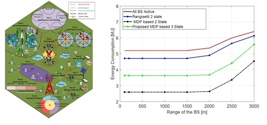
7. Simulation Results and Performance Analysis

The traffic model as presented in Section 3 is used to determine the total number of users in the coverage area of the BS at each decision epoch under the above mentioned propagation channel environment. We use Matlab to simulate our proposed algorithm. The Markov decision process along with the value iteration algorithm is used to find the required number of active, stand-by and sleeping base stations. The total observation period is 3600 s and the simulation parameters are given in Table 2. The simulation has been run for 10,000 iteration and then the average of the results are taken. The algorithm takes approximately 18,700,000 addition operation, 23,320,000 subtraction operation, 20,830,000 subtraction operation, 3,510,000 division operation and 2,900,000 logical AND operation to complete the 10,000 iteration. For the set of parameters provided in Table 2, we have found the transition probability matrix for the second BS (BS2) as the Equation (9) and the transition probabilities for the third base station(BS3) are shown in Figure 5.

$$P{r}^2=\left[\begin{array}{ccc}P{r}_{00}^2& P{r}_{01}^2& P{r}_{02}^2\\ P{r}_{10}^2& P{r}_{11}^2& P{r}_{12}^2\\ P{r}_{20}^2& P{r}_{21}^2& P{r}_{22}^2\end{array}\right]=\left[\begin{array}{ccc}0.9842& 0.0158& 0\\ 0.0044& 0.9956& 0\\ 0& 0& 0\end{array}\right]$$

(9)

For our proposed model, BS2 is capable of moving only between stand-by mode and active mode depending on the traffic condition. For the third BS, the transition among all of the three states can be presented as Figure 5. In this figure, $S_0$, $S_1$ and $S_2$ represents the states of the base station (BS3) at sleep mode, stand-by and active mode respectively; and $a_0$ and $a_1$ represent the action of BS2 becoming stand-by and active respectively.

Figure 6 compares the power consumption of the network for always active BSs referred as ‘All BS Active’; 2-state model proposed in [5] referred as ‘Rangisetti 2 state (active-standby) model’; MDP-based 2-state model [2] referred as ‘MDP-based 2 state (active-sleep) model’; and our proposed 3-state MDP model referred as ‘proposed MDP-based 3 state model’. These models can be defined as below:

• All BS Active: where all of the BSs of the network are always active.
• Rangisetti 2 State (active-standby) Model: The BSs are capable of switching between active mode and stand-by mode [5].
• MDP-based 2 State (active-sleep) Model: The BSs are capable of switching between active mode and sleep mode [2].
• Proposed MDP-based 3 State Model: The BSs are capable of switching among active mode, stand-by mode and sleep mode.

The plots clearly show that using the proposed MDP model, we can save a significant amount of power than ‘All BS active’ and ‘Rangisetti 2 state model’ in low traffic condition. This is because, as per our proposed model, some of the BSs are in active mode, one of them is in stand-by mode and rest of them are in sleep mode; whereas in ’Rangisetti 2 state model’ all of the unused BSs are in stand-by mode, which causes higher energy consumption. However, our proposed MDP-based 3 state model consumes bit more energy than the ‘MDP-based 2 state model’, that is because ‘Combes Model’ put all of the unused BSs in sleep mode only, which results in less power consumption compared to our proposed model but causes more wake up delay. This wake up delay can cause some call drops for some new users who would need to wait for a sleeping BS to wake up. However, as expected, the power consumption is the same for the two states and three states models in higher traffic condition, as almost all of the BSs needs to be active in order to support the load. In order to see the delay performance of the above mentioned four different models we generate Figure 7, which shows the percentage of the total users experiencing delay (from delay group defined in Table 3) in receiving service within the observation period for the four different models. As expected, all the users in ‘All BS active’ model will have no delay (delay group-1) at all because all of the BSs are always active for this mode. On the other hand, ‘Rangisetti 2 state model’ uses stand-by mode for the unused BSs and ‘our proposed model’ uses standby and sleep mode for the unused BSs. Therefore only a few (around $12\%$) of the users experience approximately 30 $\mathsf{\mu }$s (delay group-2) of delay for both of these models. It is noteworthy that as per the proposed MDP-based 3 state model, the users will experience delay only when a base station will have transition from stand-by to active mode. The time needed for the sleeping BS to go to stand-by mode will not cause delay to the users. Note that as per, Rangisetti model, the delay is also caused by the transition between stand-by to active mode. That is why the delay for ‘Rangisetti 2 state model’ and ‘proposed 2 state model’ are the same. On the contrary, these users (around 12%) experience 40 s (delay group-3) of delay in the ’MDP model’ as this model implements only sleep mode for unused BSs, and it takes more time for the BSs to go from sleep mode to active mode. Therefore, our proposed model offers a fair share of energy efficiency and delay in low traffic condition.

Effect of the Parameter Variation

We apply trapezoidal numerical integration [17] on the power consumption curves in order to find the total energy consumption of the network. We find that the MDP-based three state model can reduce approximately $40\%$ energy consumption compared to the ‘All BS active’ model. However, as one can expect from the power consumption curves, our proposed model is consuming little bit more energy than the MDP-based 2 state model, but this disadvantage is outweighed by the benefits of reduced delay compared to the Combes model. In this section, we vary the different parameters and have shown their effect on the energy consumption of the BS. At first, we vary the coverage range of the BS and find that the energy consumption increases rapidly after a certain range in Figure 8. For the set of parameters we have used as in Table 2, we find that the energy consumption remains almost constant for up to BS range of 1.5 km, however increases very rapidly for higher BS ranges. This scenario is true for all of the models we have used. These results depict that our proposed model consumes less energy than ‘All TRC active’ model and ’Rangisetti 2 state (active-standby) model’, however consumes little more energy than ‘MDP-based 2 state (active-sleep) model’. Figure 9 shows the expected delay experienced by the users, from where we can see that ‘MDP-based 2 state (active-sleep) model’ offers more delay than ‘Proposed 3 state model’ and ‘Rangisetti 2 state (active-standby) model’. As per the proposed MDP-based 3 state model, the users will experience delay only when a base station will have transition from stand-by to active mode. The time needed for the sleeping BS to to go stand-by will not cause delay to the users. Note that as per, Rangisetti model, the delay is also caused by the transition between stand-by to active mode. That is why the delay for ‘Rangisetti 2 state model’ and ‘proposed 2 state model’ are the same. As expected the delay increases with the BS range; however after a certain range when most of the BSs are active then the activation delay reduces. Please note that different ranges of BSs represent different types of BS (Pico, Femto, Micro, Macro etc). Figure 8 and Figure 9 provide us a good evidence to claim that our proposed model offers a fair share of energy efficiency and wake-up delay for any type of BSs.

We also observe the effect of different pathloss exponent and shadowing variance on the energy consumption (for macro BS as an example) and expected delay and the results are shown in Figure 10, Figure 11 and Figure 12 respectively. As we can expect, energy consumption of the BS increases with the path loss exponent and shadowing variance, which is clearly depicted in the figures. Figure 12 depicts that ‘MDP-based 2 state (active-sleep) model’ offers higher delay than ‘Proposed 3 state model’ and ‘Rangisetti 2 state (active-standby) model’. All of these results again show that our proposed model is an efficient model which offers a fair share of reduced energy consumption as well as reduced wake-up delay.

8. Conclusions

In this paper, we propose a novel strategy to implement sleep mode in the base stations within a multi-tier 5G network using the Markov Decision process. The proposed method considers a three-state base station model with active, sleep and standby modes where the states are adopted between each other based on the MDP-based algorithm. In the MDP-based approach we have proposed a novel reward function, which helps us to find the optimal policy depending on the traffic condition and QoS requirement to improve the energy efficiency. The results are compared with other state-of-art algorithms, from where we find that ‘MDP-based 2 state (active-sleep) model’ offers the lowest energy consumption, but the highest amount of delay. Whereas, ‘Rangisetti 2 state (active-standby) model’ reduces this delay but increases the energy consumption significantly. On contrary, Our proposed MDP bases 3 state model offers a fair share of energy efficiency and delay, where the network can save a good amount of energy when compared to Rangisetti 2 state model with ignore-able delay compared to MDP-based 2 state model. Therefore the proposed model has proven to offer a good trade-off between the energy efficiency and delay. Our future work is focused on considering the effect of interference introduced in HetNet and updating the algorithm to incorporate the effect of interference. Moreover, a stochastic geometry based energy efficiency analysis is also expected to be done as part of the future work.

References

1. Sofi, I.B.; Gupta, A. A survey on energy efficient 5G green network with a planned multi-tier architecture. J. Netw. Comput. Appl. 2018, 118, 1–28. [Google Scholar] [CrossRef]
2. Combes, R.; Elayoubi, S.E.; Ali, A.; Saker, L.; Chahed, T. Optimal online control for sleep mode in green base stations. Comput. Netw. 2015, 78, 140–151. [Google Scholar] [CrossRef]
3. Zhang, J.; Xu, L.; Zhou, S.; Ye, X. A novel sleep scheduling scheme in green wireless sensor networks. J. Supercomput. 2015, 71, 1067–1094. [Google Scholar] [CrossRef]
4. Peng, J.; Hong, P.; Xue, K. Stochastic analysis of optimal base station energy saving in cellular networks with sleep mode. IEEE Commun. Lett. 2014, 18, 612–615. [Google Scholar] [CrossRef]
5. Rangisetti, A.K.; Tamma, B.R. Interference and QoS aware cell switch-off strategy for software defined LTE HetNets. J. Netw. Comput. Appl. 2019, 125, 115–129. [Google Scholar] [CrossRef]
6. Zhang, Y.; Budzisz, L.; Meo, M.; Conte, A.; Haratcherev, I.; Koutita, G.; Tassiulas, L.; Marsan, M.A.; Lambert, S. An overview of energy-efficient base station management techniques. In Proceedings of the 2013 24th Tyrrhenian International Workshop on Digital Communications-Green ICT (TIWDC), Genoa, Italy, 23–25 September 2013; pp. 1–6. [Google Scholar]
7. Baek, S.; Song, J.J.; Choi, B.D. Performance analysis of push-to-talk over IEEE 802.16e with sleep mode and idle mode. Telecommun. Syst. 2011, 47, 291–302. [Google Scholar] [CrossRef]
8. De Vuyst, S.; de Turck, K.; Fiems, D.; Wittevrongel, S.; Bruneel, H. Delay versus energy consumption of the IEEE 802.16e sleep-mode mechanism. IEEE Trans. Wirel. Commun. 2009, 8, 5383–5387. [Google Scholar] [CrossRef]
9. Kong, L.; Wong, G.; Tsang, D. Performance study and system optimization on sleep mode operation in IEEE 802.16e. IEEE Trans. Wirel. Commun. 2009, 8, 4518–4528. [Google Scholar] [CrossRef]
10. Lui, Z.; Zhang, C.; Dong, M.; Gu, B.; Ji, Y.; Tanaka, Y. Markov-decision-process-assisted consumer scheduling in a networked smart grid. IEEE Access 2017, 5, 2448–2458. [Google Scholar]
11. Lui, Z.; Cheung, G.; Ji, Y. Optimizing distributed source coding for interactive multiview video streaming over lossy networks. IEEE Trans. Circuits Syst. Video Technol. 2013, 23, 1781–1794. [Google Scholar]
12. Saker, L.; Elayoubi, S.; Chahed, T. Minimizing energy consumption via sleep mode in green BS. In Proceedings of the 2010 IEEE Wireless Communication and Networking Conference, Sydney, NSW, Australia, 18–21 April 2010; pp. 1–6. [Google Scholar]
13. Proakis, J.G.; Salehi, M. Fundamentals of Communication Systems Paperback, 1st ed.; Prentice Hall: Englewool Cliffs, NJ, USA, 2004. [Google Scholar]
14. Gomez, K.; Sengul, C.; Bayer, N.; Riggio, R.; Rasheed, T.; Miorandi, D. MORFEO: Saving energy in wireless access infrastructures. In Proceedings of the 14th International Symposium and Workshops on World of Wireless, Mobile and Multimedia Networks (WoWMoM), Madrid, Spain, 4–7 June 2013; pp. 1–6. [Google Scholar]
15. Holtkamp, H.; Auer, G.; Bazzi, S.; Haas, H. Minimizing BS power consumption. IEEE J. Sel. Areas Commun. 2014, 32, 297–306. [Google Scholar] [CrossRef]
16. Auer, G.; Giannini, V.; Desset, C.; Godor, I.; Skillermark, P.; Olsson, M.; Imran, M.A.; Sabella, D.; Gonzalez, M.J.; Blume, O.; et al. How much energy is needed to run a wireless network? Wirel. Commun. IEEE 2011, 18, 40–49. [Google Scholar] [CrossRef]
17. Atkinson, E.K. An Introduction to Numerical Analysis, 2nd ed.; John Wiley & Sons: New York, NY, USA, 1989; ISBN 978-0-471-50023-0. [Google Scholar]
18. Ethier, S.N.; Kurtz, T.G. Markov Processes: Characterization and Convergence; John Wiley & Sons: Hoboken, NJ, USA, 2009; Volume 282. [Google Scholar]
19. Puterman, M. MPDes: Discrete Stochastic Dynamic Programming; Wiley: Hoboken, NJ, USA, 1994. [Google Scholar]
Figure 1. Multi-tier architecture for energy efficient 5G networks [1].
Remotesensing 11 01019 g001
Figure 2. Graphical representation of energy saving and energy wasting due to activating BS from sleep mode.
Remotesensing 11 01019 g002
Figure 3. Time measurement for switching between sleep mode and active mode (source: [14]).
Remotesensing 11 01019 g003
Figure 4. Proposed Three-state Markov Model for n t h base station where 2 n N . (note: The 1 s t BS is always active).
Remotesensing 11 01019 g004
Figure 5. Three-state Markov Model for BS3.
Remotesensing 11 01019 g005
Figure 6. Power consumption of the network for different models.
Remotesensing 11 01019 g006
Figure 7. Percentage of users experiencing delay.
Remotesensing 11 01019 g007
Figure 8. Effect of varying the range of the BS.
Remotesensing 11 01019 g008
Figure 9. Delay experienced by users.
Remotesensing 11 01019 g009
Figure 10. Effect of varying pathloss exponent.
Remotesensing 11 01019 g010
Figure 11. Effect of varying variance of shadowing.
Remotesensing 11 01019 g011
Figure 12. Delay experienced by users for various shadowing effect.
Remotesensing 11 01019 g012