Article

SAR Backscatter and InSAR Coherence for Monitoring Wetland Extent, Flood Pulse and Vegetation: A Study of the Amazon Lowland

1
Canada Centre for Mapping and Earth Observation, 560 Rochester St., Ottawa, ON K1A 0E4, Canada
2
MDA Corporation, Suite 201-57 Auriga Drive, Ottawa, ON K2E 8B2, Canada
3
Greenpeace Brazil, Rua Fradique Coutinho, 352 - Pinheiros, São Paulo - SP, CEP 05416-000, Brazil
*
Authors to whom correspondence should be addressed.
Remote Sens. 2019, 11(6), 720; https://doi.org/10.3390/rs11060720
Submission received: 8 February 2019 / Revised: 8 March 2019 / Accepted: 18 March 2019 / Published: 26 March 2019
(This article belongs to the Special Issue Remote Sensing Water Cycle: Theory, Sensors, Data, and Applications)

Abstract

:
Synthetic aperture radar (SAR) data have been identified as a potential source of information for monitoring surface water, including open water and flooded vegetation, in frequent time intervals, which is very significant for flood mapping applications. The SAR specular reflectance separates open water and land surface, and its canopy penetration capability allows enhanced backscatter from flooded vegetation. Further, under certain conditions, the SAR signal from flooded vegetation may remain coherent between two acquisitions, which can be exploited using the InSAR technique. With these SAR capabilities in mind, this study examines the use of multi-temporal RADARSAT-2 C band SAR intensity and coherence components to monitor wetland extent, inundation and vegetation of a tropical wetland, such as Amazon lowland. For this study, 22 multi-temporal RADARSAT-2 images (21 pairs) were used for InSAR processing and the pairs in the low water stage (November, December) showed high coherence over the wetland areas. The three-year intensity stack was used for assessing wetland boundary, inundation extent, flood pulse, hydroperiod, and wetland vegetation. In addition to the intensity, derived coherence was used for classifying wetland vegetation. Wetland vegetation types were successfully classified with 86% accuracy using the statistical parameters derived from the multi-temporal intensity and coherence data stacks. We have found that in addition to SAR intensity, coherence provided information about wetland vegetation. In the next year, the Canadian RADARSAT Constellation Mission (RCM), will provide more data with frequent revisits, enhancing the application of SAR intensity and coherence for monitoring these types of wetlands at large scales.

Graphical Abstract

1. Introduction

As for other tropical wetlands, Amazon wetlands provide many services for society, such as water storage, stabilize river discharge, groundwater recharge, organic carbon storage, withholding sediment, ecotourism, timber production, medicinal plants, agricultural products, fish, drinking water, and grazing land [1]. Furthermore, they provide homes for traditional communities and contribute significantly to biodiversity [1]. Spatial and temporal variability of flood pulse influence the inundation patterns in the floodplain, which influence the productivity and diversity of floodplain biota throughout the Amazon wetlands [2]. There is a need for understanding the behavior of the wetlands in the Amazon as the freshwater resources are becoming increasingly affected by various reasons. Increasing population, agricultural irrigation, deforestation, human interference, sedimentation, salinization and pollution are some of the possible reasons that affect the sustainability of the wetlands. More specifically, wetlands are the most vulnerable landscape feature subject to climate change [3]. As wetlands are among the most threatened ecosystems, both their regular inventory and efforts for their protection are highly recommended [1,4]. Hence, wetland ecosystems and services provided by these ecosystems require constant monitoring.
Monitoring surface water can provide critical information for wetland management. Synthetic Aperture Radar (SAR) has been shown to be excellent for surface water monitoring, largely for open water [5]. This has led to a variety of intensity thresholding schemes for mapping open water [6,7,8,9]. SAR also has shown its potential for monitoring water under vegetation canopies, with its penetration and double bounce capabilities [10,11,12,13,14]. Based on that, a variety of SAR techniques have been developed for identifying flooded vegetation, including intensity thresholds, polarimetric decomposition, and InSAR coherence [15]. The enhanced backscatter intensity of some polarizations allows one to use bright target thresholding techniques for identifying flooded vegetation [10,11,12,13,14,15,16,17,18,19]. Recent studies have used InSAR technology to monitor water level changes in a variety of wetlands, including tropical wetlands in the Amazon, the mangroves and sawgrass marshes of the Everglades, flooded forest in the central Congo Basin, and hardwood swamps in Louisiana [20,21,22,23,24,25,26,27,28,29]. Suitable coherence has been observed at X, C, and L-band frequencies, although the maintenance of coherence during the temporal data acquisition period is critical to this methodology. In tropical floodplains like the Amazon, often the water level is high and inundate wetland vegetation that makes significant areas as temporary open water [30]. This is also a factor in addition to the common factors, such as perpendicular baseline, temporal baseline, change in water level, high biomass, target motion, change in dielectric constant, and atmospheric conditions [31,32,33,34], which disturb the coherence of phase over wetlands inconsistent over time limiting the use of the InSAR technique for water level monitoring.
SAR satellites, such as ALOS PALSAR, RADARSAT-2, COSMOS Sky-Med, Terra-SAR/X, Sentinel-1, and upcoming RADARSAT Constellation Mission (RCM), provide timely data for dynamic wetland monitoring activities. Further, their advanced capabilities, such as interferometric data with short temporal baselines, polarimetric data, high resolution data, and single or dual pol standard mode consistent data products offer exciting possibilities for identifying innovative methods for wetland, flooded vegetation and water resource applications [34,35,36]. This study follows a wetland monitoring study near Ottawa, Ontario conducted by the Canada Centre for Remote Sensing (CCRS) using RADARSAT-2 data acquired in 2011-2013. The previous study showed the use of coherence and intensity from a stack of RADARSAT-2 for characterizing the wetlands in the temperate ice-off season [34]. This paper reports an investigation of the use of intensity and/or coherence from a stack of RADARSAT-2 images acquired in 2014-2016 for wetland extent, flood pulse and hydroperiod in the Amazon tropical floodplain region throughout the high and low water stages. The knowledge gained from tropical and temperate wetlands will be used to propose a methodology that could lead to the use of RADARSAT-2 and RCM data for wetland monitoring.

2. Study Area Characteristics

Study Area Description

The study area is part of the lower Amazon floodplain in the State of Pará, Brazil (Figure 1) consisting of a complex Amazon river network, lakes and floodplains. The lower Amazon floodplain is classified as várzea, a type of floodplain that are periodically flooded by sediment-rich white-water rivers of the Amazon [2,37]. The level of water in the area varies seasonally throughout the year in response to the spatial and temporal distribution of rainfall in the Amazon catchment [38]. These seasonally fluctuating water levels are known as ‘flood pulses’ [1,2]. These flood-pulses [2] are different for most of the wetlands in tropics, sub-tropics, and temperate region. The average amplitude of flood pulses can exceed 10 m in the Amazon River, depending on the location and the amount of rainfall [1]. Based on [1], mean flood pulse amplitude at the Santarém station (Figure 1) in the study area is about 4 m with a maximum water level in June and a minimum in November.
The vegetation composition of várzea wetland forests, swamps, and wet savannas is strongly dependent on the amplitude of the flood-pulse [39]. These flood-pulsing wetlands are covered by woody and herbaceous plants, which have a large ecological tolerance of flood and drought stress [1]. Different forest types become established in relation to the flood-level gradient [40] and the formations are characterized by typical patterns of species composition, and their architecture. The herbaceous plant species usually grow from seed banks in the sediments or from vegetative resting stages during the flooding phase [1]. Extended communities of fast growing and free-floating aquatic macrophytes develop at rising waters over the areas that are mostly occupied by annual grasses, sedges, and herbs during low water stages [1]. Fishes, aquatic birds, insects, reptiles, amphibians, and mammals tend to recolonize temporary wetlands by emigration from permanently aquatic habitats [1]. Further, the flood level influences the dynamics of fish populations and associated fishery yields [2].

3. Data and Methods

3.1. RADARSAT-2 Data

Our previous research demonstrated that high resolution (1–5 m) C-HH data were well suited for interferometry [41]. Based on that, extra fine mode (XF0W2) right looking ascending pass RADARSAT-2 C-HH data were acquired in 2014-2016 covering 139 x 71 km2 of Amazon floodplain centered 54.9017° W, 2.1173° S. All 22 scenes of XF0W2 Single Look Complex (SLC) data were acquired (Table 1) with an incident angle of about 35° and a pixel spacing of 2.6 m in range and 2.5 m in azimuth in slant range projection. Besides, Shuttle Radar Topography Mission (SRTM) 1 void filled elevation data at a resolution of 1 arc-second (30 meters) was used for orthorectification and further analysis (https://lta.cr.usgs.gov/SRTM1Arc). As shown in Figure 2 these data sets were processed and used for extracting wetland boundary, surface water/inundation extent, flood pulse, hydroperiod, and wetland vegetation.

3.2. SAR and InSAR Processing

Gamma Remote Sensing software and in-house tools were used for the InSAR processing to derive backscatter and coherence images. The InSAR processing combines two SLC SAR images into an interferogram. Due to temporal de-correlation of the vegetation and rapid water level changes in Amazon floodplain, processing was done only with the next available InSAR pair. The minimum and the maximum temporal baseline of the RADARSAT-2 pairs used in this study is 24 days and 120 days respectively. The radar products were co-registered and the interferograms, which measures the phase displacement of targets between the two dates, were generated from all of the next available InSAR pairs [34]. The interferogram, coherence and multi look SAR backscatter products were generated and then orthorectified. The generated coherence, is a measure of decorrelation of two co-registered acquisitions, has a range of values of 0.0 to 1.0 [34]. Further, temporal intensity and coherent stacks were created and statistical products, such as minimum, maximum, mean, standard deviation and skewness were derived from RADARSAT-2 intensity and coherent stacks using IDL programming.

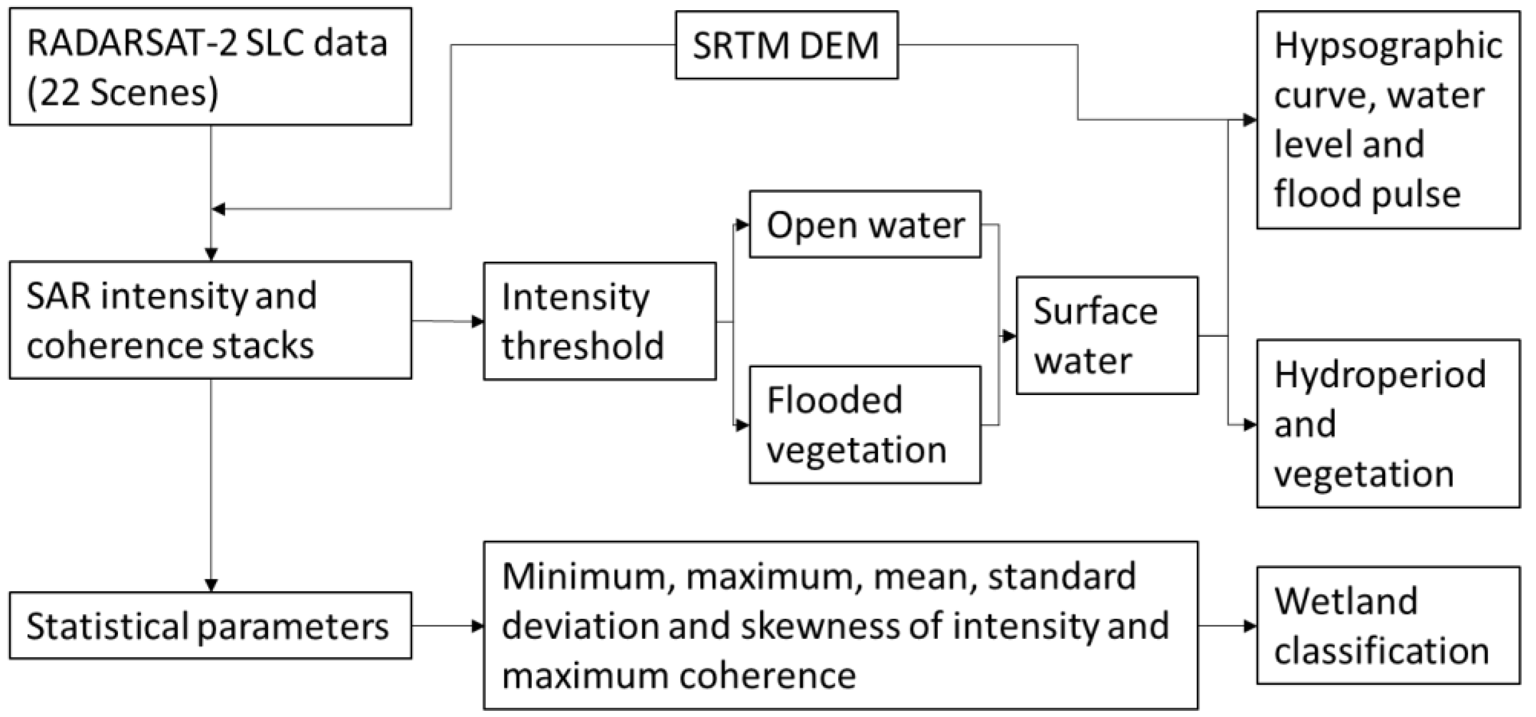
3.3. Open Water and Flooded Vegetation Extraction

Low intensity thresholding method was used to mask open water from the radar backscatter image [15]. To determine the threshold (dB), image histogram and obvious open water samples were used. Although all the images are HH polarized and have nearly identical incidence angles, the selection of the open water threshold was scene specific because of weather conditions and near range effects. There is occasionally an increase in backscatter because of the waves present in water, which can cause omission of open water. In order to minimize the error, due to the wind effect, extracted open water images (bitmap images) were manually examined and edited if required. Out of 22, four open water images, which were acquired on 11 Oct 2014, 04 Mar 2015, 06 Oct 2015 and 17 Dec 2015 were identified and edited to remove the relatively bright patches over the open water area at the near range side of the images. Similarly, the flooded vegetation mask was based on high intensity threshold and the cities with high intensity were removed from the flooded vegetation images (bitmap images). All these processes were done using PCI Geomatica software.

3.4. Multi-Temporal SAR Classification

Unsupervised classification of six statistical parameters, that include minimum, maximum, mean, standard deviation, skewness of intensity and maximum of coherence, was done using PCI software. Initially, 30 classes were classified using k-mean unsupervised classification algorithm and regrouped to nine classes based on the visual interpretation of pan-sharpened Landsat TM images acquired during the 3 years period (04 Sep 2014, 13 Jun 2015, 14 Aug 2015, 17 Oct 2015, 18 Nov 2015, 04 Dec 2015, 20 Dec 2017, 16 Aug 2016), Google earth and Bing maps. The classified output was subjected to accuracy assessment. Over the extent of the classified map, 200 random samples were generated using ARCmap software. The points were overlaid on the Google earth, Bing maps and pan-sharpened Landsat TM images, and the land cover type of each point were identified. Then the points belong to the classes were extracted from the classified image. With those 200 justification points, a confusion matrix was created and overall accuracy and omission and commission errors and the Kappa coefficient were calculated.

4. Results and Discussion

In this section, we have summarized the products or information that can be extracted from multi-temporal RADARSAT-2 HH intensity and coherence data and discussed the impact of the derived information for natural resource and environmental applications, such as protected area, flooding, fisheries, forestry and lifecycle of flora and fauna.

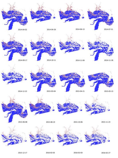
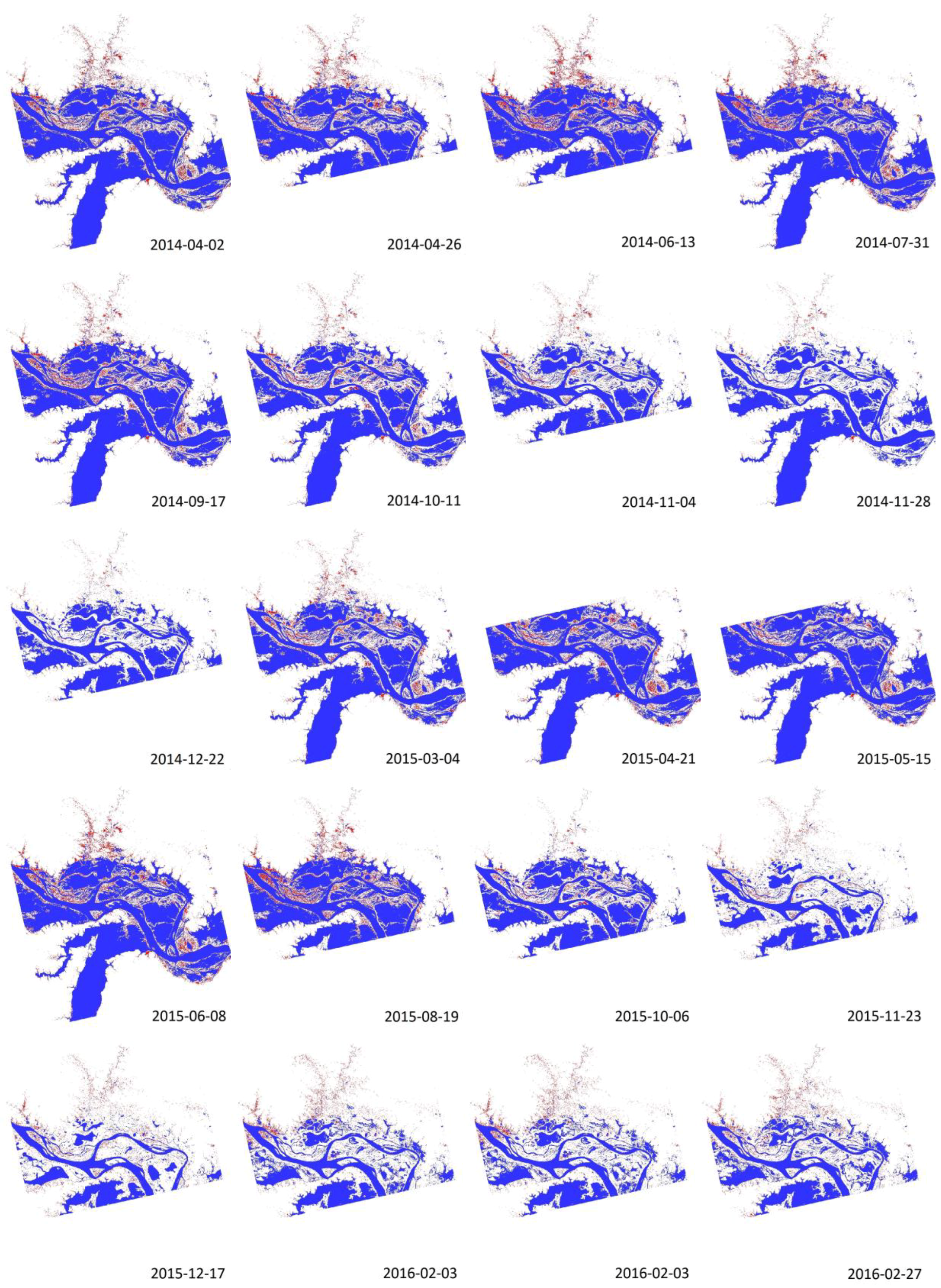
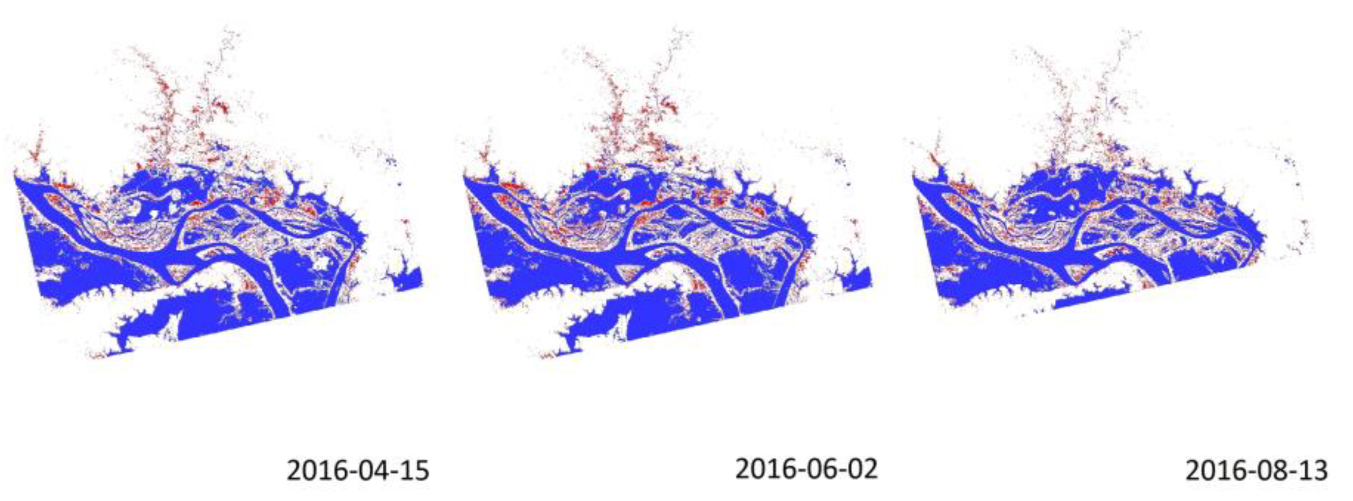
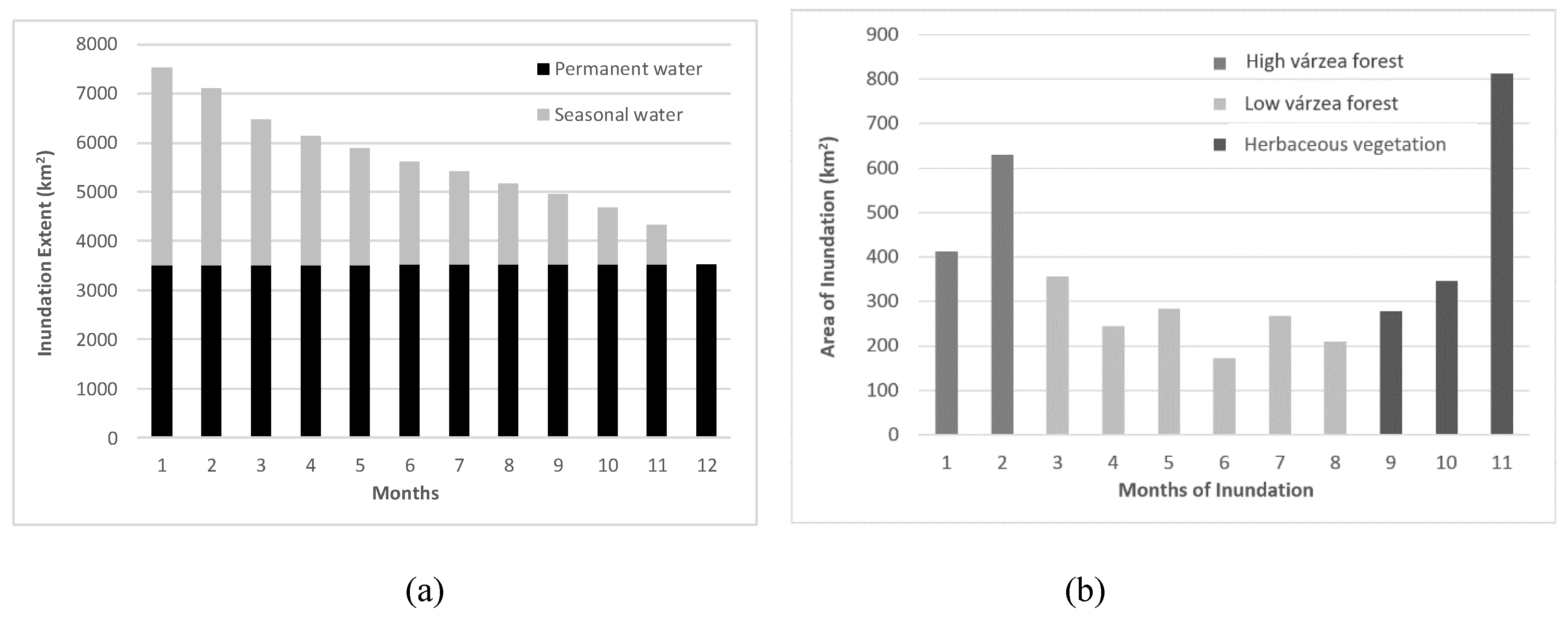
4.1. Inundation Extent

The wetland inundation extent plays a key role in ecosystem dynamics [42,43]. The inundation extent of wetlands is one of the largest uncertainties in applying models of wetland function [38,42]. This has long been recognized in the International Geosphere Biosphere Programme Global Analysis, Integration and Modeling report, which states “Wetland extent: The largest gap in wetland characterization is the size of wetlands themselves, both in space and time” [42]. Initially, [44] estimated the water extent over the Amazon, at low and high water stages, from SAR data. With the emerging high spatial and temporal resolution of SAR data, it is now feasible to monitor seasonal and inter-annual variation [6] in inundation extent, for example, to evaluate how this variation influences greenhouse gas exchanges in the region.
Figure 3 shows the inundation extent, which was derived over the 2014–2016 time period using RADARSAT-2 images using the methodology described in Section 3.3. As shown in Figure 3, the open water (blue color) is classified based on low intensity threshold and the flooded vegetation (red color) is classified based on high intensity threshold [15]. The results showed that intensity thresholding can be used to extract open water and flooded vegetation to map wetlands over a large area like the Amazon várzea. It is important to note that the user selection of the intensity threshold approach sometimes can introduce uncertainty that can be rectified using automated or manual cleanup process [45,46]. As described in the methodology, relatively bright patches over the open water area at the left (near range) side, due to the wind effect were removed from 11 Oct 2014, 04 Mar 2015, 06 Oct 2015 and 17 Dec 2015 images. It is also possible to identify and omit these images, when we get very frequent images from RCM. The advantage here is that it captured the dynamic changes in the surface water extent (Figure 3), which is very useful for wetland monitoring [42]. During high water stage (March to August), the inundation extent is very large compared to low water stage (September to February) and particularly the flooded vegetation area is significant as the water reach higher levels and inundate the permanent vegetation areas. The net loss or net gain of surface water area from the observation period provide a spatial snapshot of the water cycle and highlight which areas had an increase or decrease in water extent (Figure 3). Based on [47], methane emission and CO2 sink respond to the changes in wetland inundation extent. Change in surface water extent also shows the hydromorphic processes that can permanently modify wetland surfaces through erosion and sediment deposition that affects biotic community development [37,39].

4.2. Flood Pulse

In the Amazon várzea, hydrology is the major driving force and can be interpreted using flood pulse. Amplitude, duration, shape, frequency, timing, and predictability are all important characteristics of the flood pulse [39]. One of the attributes of the flood pulse is to regulate the limnological, physical and chemical characteristics of contiguous water bodies by increasing hydrological connectivity [37]. The hydrological connectivity supports the water-mediated transport of matter, energy and organisms within or between the components of the hydrological cycle [37]. Changes in elevation of a few decimeters or meters can considerably modify the impact of the flood pulse and increase habitat diversity [39].
As the flood pulse of a specific location is an important indicator for hydrology and biodiversity, we estimated the flood pulse using surface water products derived from remote sensing. For that, the elevation of the water level was estimated from the surface water extent assuming a flat water surface. This is based on the hypsographic curve [48] showing the relationship between the elevation and the area less than the particular elevation of the selected cross section area (Figure 4a) of the river valley using the SRTM DEM. Figure 4b shows the relationship that was used to estimate the water level from the surface water extent.
Figure 5a shows the temporal pattern of the estimated water level based on the SAR derived surface water area (Figure 3) that includes open water and flooded vegetation. The water level of a particular date is calculated from the SAR derived surface water area of the same cross section that is shown in Figure 4a using the derived power equation (Figure 4b). The flood pulse from 3 years of data (Figure 5a) shows a comparable annual flood pulse pattern developed from the hydro station hourly water level data of Santarém station (2°25.93′ S, 54°41.45′ W), which is in the study area and close to the selected cross section. Though the pattern is allied and the estimated and observed water levels are highly correlated (R2 = 0.9), the water level is under estimated that is about 46% (Figure 5b) of the observed water level. The error could be because of three reasons: (1) The accuracy of the SRTM DEM; (2) systematic underestimation of open water and flooded vegetation; and (3) difference between the cross section and the hydro station locations. The SRTM DEM is relatively accurate. However, there is a possibility to have low absolute elevation accuracy predominantly in the low elevation floodplain area. At this moment, we do not have any means to validate the absolute elevation of the SRTM DEM. The cross section is away from the hydro station location because only nine images out of 22 cover the Santarém area (see Figure 3) that is not adequate for showing flood pulse. Further, the correlation between the estimated and observed water levels at rising and recession limbs are different (Figure 5c). There is a 0.5 m underestimation during the water level rising limb. This variation may be due to the time lag (an average of 25 days) between the water level raise at the river and the flooding at the far end of ~35 km wide floodplain. Moreover, a very high correlation between the estimated and observed water level at rising (R2 = 0.99) and recession (R2 = 0.98) limbs (Figure 5c) pronounce the correctness of the surface water extraction from SAR.
However, this annual pulse, the periodic change between a terrestrial and an aquatic water phase, is the most important factor affecting plant fitness in Amazonian várzea wetlands. Usually these phases are important for biotic population maintenance [37]. In the case of aquatic herbaceous vegetation, the flood pulse changes the availability of habitats and nutrients throughout the year, influencing the spatial distribution and the percentage of surface covered by their populations [37]. This flood pulse controls the productivity of fisheries in the study area. High and low water indices, which are calculated as the area under and above the hydrograph curve relative to a ‘bank-full’ level, in any given year affects fishery yields two and three years later [2].

4.3. Hydroperiod

In temporary freshwater ecosystems, hydroperiod (inundation duration) is commonly found to be one of the fundamental factors affecting community structure and it is generally found that species richness increases with inundation duration [49]. As inundation duration increases, larger and longer-lived species can be supported and it also favors the expansion of the coverage area of floating herbaceous vegetation [37]. Figure 6 is a hydroperiod map developed from the surface water maps, which includes open water and flooded vegetation (Figure 3). This was created based on the frequency of the number of times a pixel is identified as water in the multiple surface water maps. Then the frequency (1-22) was converted to months (1-12) assuming the surface water maps are equally spaced in time for simplifying interpretation. This assumption will be more valid when we use very frequent SAR data from forthcoming RCM satellites. This map can be used for understanding wetland functions and for applying models of wetland functions, where the temporal and spatial extent of wetland flooding should be characterized in terms of hectare-days [42]. Figure 7a which was derived from Figure 6 area statistics shows such values (area is in gray: km2-months) of the study area and can be used for such models.
This map can also be used for the zonation of plant communities described in [37]. According to Ferreira’s zonation [37], the vegetation zonation along the hydroperiod and flood-level gradient on várzea floodplains are well characterized. Central Amazonian várzea forests are divided as high várzea or low várzea, with few species found in both forest types. High várzea forests are found on more stable sites, where the flood period is generally < 50 days per year and the water level is <3 m. Low várzea forests become established where the annual water column has an average height of >3 m, which corresponds to an inundation period of 50 to 270 day per year. The herbaceous vegetation is subjected to average annual flooding of 8–9 months. Figure 7b which was derived from Figure 6 shows the area statistics of wetland vegetation of the study area based on the Ferreira’s zonation. Although, the vegetation composition of the várzea floodplain depends on the duration and amplitude of flooding, the derived three zones are not detailed enough to categorize the actual wetland vegetation.

4.4. Wetland Vegetation

In this section, we included the coherence, calculated by correlating the RADARSAT-2 scenes in pairs for classifying wetland vegetation. Figure 8 shows all the 21 coherence products and specifically shows the coherence of 23 November and 17 December 2015 scenes separated by 24 days. The SAR response signal from flooded vegetation remained coherent during that repeat satellite over-passes, as also observed by [50]. The coherence increases with the vertical or near-vertical vegetation component above the water surface that provides double-bounce reflection. In addition, river sand banks can also show high coherence, as also reported by [32]. The high coherence within the wetland boundary that is shown in yellow color was from the flooded vegetation or sometimes the sand shore. Here, upland agriculture also shows high coherence but that is not our interest. Motion of the vegetation caused by wind and growth, changes in the dielectric constant of the vegetation, and very high water level changes between the two dates decrease coherence, which is more common for C band SAR [34]. Therefore, we experienced low coherence over flooded vegetation for a number of pairs that limits the use of the coherence alone for wetland classification in this study.
In order to understand the vegetation composition of the Amazon várzea floodplain statistical products derived from RADARSAT-2 intensity and coherent stacks, which gives meaningful information for wetland classification, were used. These products were:
  • Minimum intensity—information on open water area
  • Maximum intensity—information on flooded vegetation
  • Mean intensity—information on land surface
  • Standard deviation of intensity—information on change
  • Skewness of intensity—information on pattern of change
  • Maximum coherence—coherent for a certain period
Figure 9 shows an intensity coherence color composite that was developed from three of the above six parameters to effectively visualize the wetland area. The three channels used for Figure 9 are related to changes. Here, red represents maximum coherence, green represents the standard deviation of intensity, and blue represents skewness of intensity. This combination was selected because; the maximum coherence gives higher values for flooded vegetation, due to their high coherency at least from a single pair; standard deviation of intensity shows higher values for flooded vegetation, due to the variation between dry period and strong double bounce during flooded time; and the skewness, which characterizes the degree of asymmetry of a histogram distribution around its mean [51], shows higher values for dynamic temporary open water compare to permanent open water and land. The color composite (Figure 9) is useful for visualizing the study area and for highlighting wetlands. Upland dense forests are in dark green and with the reducing density of the forest, the color changes to green, yellow, orange and red, due to increasing coherence and may be, due to increasing openness. However, high density flooded forest in the wetland area shows in light green as it was flooded for sometimes resulting slightly higher coherence due to typical double bounce scattering. Though, the standard deviation shows a range of the changes, the skewness demonstrates the pattern of change (more or less indicating hydroperiods). Therefore, the wetland areas are shaded with a blueish tone. The magenta color indicates long duration inundated areas occasionally showing high coherence due to the strong double bounce scattering from flooded herbaceous vegetation. This demonstrates the significance of integrating coherence products with intensity products for monitoring flooded vegetation and identifying general land-cover. The color of lower part of the color composite (Figure 9) is slightly different as a few images (see Figure 3) does not cover the lower part, so the number of multi-temporal images/pixels used for the statistical products were different.
Figure 10 provides a map of wetland extent and vegetation type of the study area classified from the above six statistical products derived from RADARSAT-2 intensity and coherent stacks. The extent of the wetland visually matches with the classified image [44] that was the first validated estimate of wetland derived from the Global Rain Forest Mapping Project (GRFM) Amazon low-flood and high-flood seasons mosaics. However, our classification is comprehensive as we have used very high resolution multi-temporal intensity and coherence data for the classification. The accuracy assessment was performed as a standard error matrix (Table 2) with the help of the land cover information of 200 random validation points interpreted from Google earth and Bing maps and pan-sharpened Landsat TM images.
Though multiple high resolution images of Google earth and Bing maps cover the study area, most of the high resolution images of Google earth were acquired during high water stage and most of the high resolution images of Bing maps were acquired during low water stage. These complementary coverages helped to separate the classes without much trouble. The classes, such as settlement and agriculture/grassland, were very visible on both Google earth and Bing maps. The primary forest and degraded forest were separated based on the density of the vegetation appeared on the Google earth and Bing maps. Forests, shrubs and herbaceous within the floodplain area were identified using Bing maps and if those points were flooded or submerged based on Google earth or any of the available Landsat TM data acquired during the three year period, they were categorized as flooded forest, flooded shrubs and flooded herbaceous classes respectively. Aquatic herbaceous are prominent with bright bluish red color on Landsat TM false color composites (R,G,B: NIR,Red,Green) mainly during the low water stage. Due to lack of resources, the uncertainty of the visual interpretation is not assessed with ground data.
The overall accuracy of the SAR statistical parameters classification (Figure 10) is 86% and the Kappa coefficient is 0.83. Table 3 illustrates commission errors that represent pixels that belong to another class, but are labeled as the class and omission errors that represent pixels that belong to the class but fail to classify into the proper class. Table 3 also shows individual Kappa coefficients, a discrete multivariate technique for accuracy assessment, for each class. From the class Kappa coefficient, it is clear that out of all the classes, floodplain shrub and herbaceous are poorly classified as the two classes are naturally mixed-up. This is mainly because of the density of the shrubs that decides the classes. Similarly, in the upland area, some of the low-density open degraded forests are labeled as agriculture or grassland class. Here, floodplain forest is very well discriminated from other vegetation because of its unique interaction with SAR. However, C-band SAR has limited penetration through thick forest canopies and that categories might not be separable.
The spatial distribution of the land use/cover types of the upland area is dominated by thick forest. However, agriculture or grass patches are also significantly distributed in the study area. In the wetland area, well developed species and early secondary tree species are classified under floodplain forest [37]. Further, monospecific stands of pioneer short-lived woody perennials mixed with herbaceous plants are common in floodplain shrub [37]. Herbs and perennial grasses are typical of floodplain herbaceous. Dry period sand shores colonized by annual grasses, sedges, and semi-aquatic herbs are classified as aquatic herbaceous [37]. Some herbaceous species spread predominantly by vegetative regrowth cover the upper soil layers that prevents erosion and promotes the early stages of succession [37].

5. Conclusions

Monitoring extensive areas of wetlands represents a formidable task for water resource managers in many parts of the world. For example, in areas like the Amazon, authorities have limited capabilities for monitoring because of the dynamic nature of the wetland, accessibility, and persistent cloud cover that limits optical imaging. Remote sensing with radar offers more capabilities (weather independent, day and night acquisition, specular reflection, penetration and double bounce scattering) than optical, and SAR would permit monitoring of both long-term and rapid changes of wetlands and their interconnections across entire watersheds. In this study we have demonstrated the use of multi-temporal RADARSAT-2 satellite data for extracting wetland boundary, flood pulse, hydroperiod and vegetation.
The intensity thresholding method worked well to extract open water and flooded vegetation for mapping surface water or wetland extent of the study area, as only 4 out of 22 open water products (<20%) were edited to remove relatively bright patches over the open water area, due to the wind effect. The estimated wetland extent accuracy was prominent because the correlation between the estimated water level, which was based on the hypsographic curve using the wetland extent products, and observed water level at rising (R2 = 0.99) and recession (R2 = 0.98) limbs are were very high. However, there is a 0.5 m underestimation during the water level rising limb and the variation may be due to the time lag (an average of 25 days) between the water level raise at the river and the flooding at the far end of ~35 km wide floodplain. This time lag should be evaluated in future studies. The hydroperiod map, which can be used to characterize the temporal and spatial extent of wetland flooding in terms of hectare-days, was also created from the multiple wetland extent products. Moreover, the overall accuracy of the SAR statistical parameters classification is 86% and the Kappa coefficient is 0.83. This validation is based on the expert visual interpretation of available high resolution optical images and the uncertainty of the visual interpretation is not quantified because of a lack of resources.
Further, using similar methods, yearly flood pulse and hydorperiod map can be produced using frequently observed SAR data stacks from current and future satellites. Our interferometric analysis shows that high coherence can be obtained from wetland vegetation. However, the coherence can drop quickly when the wetland water level rapidly changes. There was major growth and change of the herbaceous vegetation in the marsh area, which made the greatest variability in coherence during the three years period. This knowledge and these applications represent the advancement in using SAR images for wetland monitoring and management. Furthermore, wetland monitoring application and techniques will be improved by using ample of data from existing SAR satellites, such as Terra-SAR/X and COSMO SkyMed, Sentinel, and the upcoming RCM, which will provide frequent revisits.

Author Contributions

Conceptualization, F.C., B.B., K.M. and M.V.; Methodology, F.C. and B.B.; Software, F.C. and K.M.; Validation, F.C. and E.K.; Formal Analysis, F.C.; Investigation, F.C., B.B., K.M. and M.V.; Resources, B.B.; Data Curation, K.M., F.C. and E.K.; Writing-Original Draft Preparation, F.C.; Writing-Review and Editing, F.C., B.B., M.V. and E.K.

Funding

This research received no external funding.

Acknowledgments

This work was supported by the Remore Sensing Science program at the Canada Centre for Mapping and Earth Observation. The authors would like to acknowledge the contribution of Frank Ahern and François Charbonneau, who provided scientific and editorial peer review of the manuscript and helpful comments to improve content.

Conflicts of Interest

The authors declare no conflict of interest.

References

  1. Junk, W.J.; Piedade, M.T.F.; Lourival, R.; Wittmann, F.; Kandus, P.; Lacerda, L.D.; Bozelli, R.L.; Esteves, F.A.; Nunes Da Cunha, C.; Maltchik, L.; et al. Brazilian wetlands: Their definition, delineation, and classification for research, sustainable management, and protection. Aquatic Con. Marian Fres. Ecos. 2014, 24, 5–22. [Google Scholar] [CrossRef]
  2. Castello, L.; Isaac, V.J.; Thapa, R. Flood pulse effects on multi species fishery yields in the Lower Amazon. R. Soc. Open sci. 2015, 2, 150299. [Google Scholar] [CrossRef]
  3. IPCC (Intergovernmental Panel on Climate Change). Climate Change and Water; Intergovernmental Panel on Climate Change. Available online: https://www.ipcc.ch/site/assets/uploads/2018/03/climate-change-water-en.pdf (accessed on 26 March 2019).
  4. SCBD (Secretariat of the Convention on Biodiversity). Global Biodiversity Outlook 3. Secretariat of the Convention on Biodiversity: Montreal, Canada. Available online: https://www.cbd.int/doc/publications/gbo/gbo3-final-en.pdf (accessed on 26 March 2019).
  5. Brisco, B.; Short, N.; Van der Sanden, J.; Landry, R.; Raymond, D. A semi-automated tool for surface water mapping with RADARSAT-1. Can. J. Remote Sens. 2009, 35, 336–344. [Google Scholar] [CrossRef]
  6. Martinez, J.M.; Le Toan, T. Mapping of flood dynamics and spatial distribution of vegetation in the Amazon floodplain using multi-temporal SAR data. Remote Sens. Environ. 2007, 108, 209–223. [Google Scholar] [CrossRef]
  7. Matgen, P.; Hostache, R.; Schumann, G.; Pfister, L.; Hoffmann, L.; Savenije, H.H.G. Towards an automated SAR-based flood monitoring system: Lessons learned from two case studies. Phys. Chem. Earth. 2011, 36, 241–252. [Google Scholar] [CrossRef]
  8. Wendleder, A.; Wessel, B.; Roth, A.; Breunig, M.; Martin, K.; Wagenbrenner, S. TanDEM-X Water Indication Mask: Generation and First Evaluation Results. IEEE J. Selec. Top. Appl. Earth Obs. Remote Sens. 2012, 6, 1–9. [Google Scholar] [CrossRef]
  9. Martinis, S.; Rieke, C. Backscatter Analysis Using Multi-Temporal and Multi-Frequency SAR Data in the Context of Flood Mapping at River Saale, Germany. Remote Sens. 2015, 7. [Google Scholar] [CrossRef]
  10. Hess, L.L.; Melack, J.; Simonett, D. Radar detection of flooding beneath the forest canopy: A review. Int. J. Remote Sens. 1990, 11, 1313–1325. [Google Scholar] [CrossRef]
  11. Kasischke, E.S.; Bourgeau-Chavez, L.L. Monitoring South Florida wetlands using ERS-1 SAR imagery. Photogramm. Eng. Remote Sens. 1997, 63, 281–291. [Google Scholar]
  12. Pope, K.O.; Rejmankova, E.; Paris, J.F.; Woodruff, R. Detecting seasonal flooding cycles in marshes of the Yucatan Peninsula with SIR-C polarimetric radar imagery. Remote Sens. Environ. 1997, 59, 157–166. [Google Scholar] [CrossRef]
  13. Townsend, P.A. Relationship between forest structure and the detection of flood inundation in forested wetlands using C-band SAR. Remote Sens. Environ. 2002, 23, 443–460. [Google Scholar] [CrossRef]
  14. Kasischke, E.S.; Smith, K.B.; Bourgeau-Chavez, L.L.; Romanowicz, E.A.; Brunzell, S.M.; Richardson, C.J. Effects of seasonal hydrologic patterns in south Florida wetlands on radar backscatter measured from ERS-2 SAR imagery. Remote Sens. Environ. 2003, 88, 423–441. [Google Scholar] [CrossRef]
  15. White, L.; Brisco, B.; Dabboor, M.; Schmitt, A.; Pratt, A. A Collection of SAR Methodologies for Monitoring Wetlands. Remote Sens. 2015, 7. [Google Scholar] [CrossRef]
  16. Horritt, M.S.; Mason, D.C.; Cobby, D.M.; Davenport, I.J.; Bates, P.D. Waterline mapping in flooded vegetation from airborne SAR imagery. Remote Sens. Environ. 2003, 85, 271–281. [Google Scholar] [CrossRef]
  17. Chapman, B.; McDonald, K.; Shimada, M.; Rosenqvist, A.; Schroeder, R.; Hess, L. Mapping Regional Inundation with Spaceborne L-Band SAR. Remote Sens. 2015, 7, 5440–5470. [Google Scholar] [Green Version]
  18. Plank, S.; Jüssi, M.; Martinis, S.; Twele, A. Mapping of flooded vegetation by means of polarimetric Sentinel-1 and ALOS-2/PALSAR-2 imagery. Int. J. Remote Sens. 2018, 38. [Google Scholar] [CrossRef]
  19. Tsyganskaya, V.; Martinis, S.; Marzahn, P.; Ludwig, R. SAR-based detection of flooded vegetation—A review of characteristics and approaches. Int. J. Remote Sens. 2018, 39, 2255–2293. [Google Scholar] [CrossRef]
  20. Alsdorf, D.; Smith, L.; Melack, J. Amazon floodplain water level changes measured with interferometric SIR-C radar. IEEE Trans. Geosci. Remote Sens. 2001, 39, 423–431. [Google Scholar] [CrossRef]
  21. Lu, Z.; Kwoun, O.I. Radarsat-1 and ERS InSAR analysis over southeastern coastal Louisiana: Implications for mapping water-level changes beneath swamp forests. IEEE Trans. Geosci. Remote Sens. 2008, 46, 2167–2184. [Google Scholar] [CrossRef]
  22. Wdowinski, S.; Kim, S.W. Space based detection of wetlands’ surface water level changes from L band SAR interferometry. Remote Sens. Environ. 2008, 112, 681–696. [Google Scholar] [CrossRef]
  23. Kim, S.W.; Lu, Z.; Lee, H.; Shum, C.K.; Swarzenski, C.M.; Doyle, T.W.; Baek, S.H. Integrated analysis of PALSAR/Radarsat-1 InSAR and ENVISAT altimeter data for mapping of absolute water level changes in Louisiana wetlands. Remote Sens. Environ. 2009, 113, 2356–2365. [Google Scholar] [CrossRef]
  24. Hong, S.H.; Wdowinski, S.; Kim, S.W.; Won, J.S. Multi-temporal monitoring of wetland water levels in the Florida Everglades using interferometric synthetic aperture radar (INSAR). Remote Sens. Environ. 2010, 114, 2436–2447. [Google Scholar] [CrossRef]
  25. Lee, H.; Yuan, T.; Jung, H.C.; Beighley, E. Mapping wetland water depths over the central Congo Basin using PALSAR ScanSAR, Envisat altimetry, and MODIS VCF data. Remote Sens. Environ. 2015, 159, 70–79. [Google Scholar] [CrossRef]
  26. Yuan, T.; Lee, H.; Jung, H.C. Toward estimating wetland water level changes based on hydrological sensitivity analysis of PALSAR backscattering coefficients over different vegetation fields. Remote Sens. 2015, 7, 3153–3183. [Google Scholar] [CrossRef]
  27. Kim, D.; Lee, H.; Laraque, A.; Tshimanga, R.M.; Yuan, T.; Jung, H.C.; Beighley, E.; Chang, C.-H. Mapping spatio-temporal water level variations over the central Congo River using PALSAR ScanSAR and Envisat altimetry data. Int. J. Remote Sens. 2017, 38, 7021–7040. [Google Scholar] [CrossRef]
  28. Yuan, T.; Lee, H.; Jung, H.C.; Aierken, A.; Beighley, E.; Alsdorf, D.; Tshimanga, R.; Kim, D. Absolute water storages in the Congo River floodplains from integration of InSAR and satellite radar altimetry. Remote Sens. Environ. 2017, 201, 57–72. [Google Scholar] [CrossRef]
  29. Cao, N.; Lee, H.; Jung, H.C.; Yu, H. Estimation of water level changes of large-scale Amazon wetlands using ALOS2 ScanSAR differential interferometry. Remote Sens. 2018, 10, 966. [Google Scholar] [CrossRef]
  30. Abril, G.; Martinez, J.M.; Artigas, L.F.; Moreira-Turcq, P.; Benedetti, M.F.; Vidal, L.; Meziane, T.; Kim, J.H.; Bernardes, M.C.; Savoye, N.; et al. Amazon River carbon dioxide outgassing fuelled by wetlands. Nature 2014, 505, 395–398. [Google Scholar] [CrossRef] [PubMed]
  31. Hagberg, J.O.; Ulander, L.M.; Askne, J. Repeat-pass SAR interferometry over forested terrain. IEEE Trans. Geosci. Remote Sens. 1995, 33, 331–340. [Google Scholar] [CrossRef]
  32. Canisius, F.; Kiyoshi, H.; Tokunaga, M. Updating geomorphic features of watersheds and their boundaries in hazardous areas using satellite synthetic aperture radar. Int. J. Remote Sens. 2009, 30, 5919–5933. [Google Scholar] [CrossRef]
  33. Olesk, A.; Antropov, O.; Zalite, K.; Arumäe, T.; Voormansik, K. Interferometric SAR coherence models for characterization of hemiboreal forests using TanDEM-X Data. Remote Sens. 2016, 8, 1–23. [Google Scholar] [CrossRef]
  34. Brisco, B.; Ahern, F.; Murnaghan, K.; White, L.; Canisius, F.; Lancaster, P. Seasonal Change in Wetland Coherence as an Aid to Wetland Monitoring. Remote Sens. 2017, 9. [Google Scholar] [CrossRef]
  35. Canisius, F.; Shang, J.; Liu, J.; Huang, X.; Ma, B.; Jiao, X.; Geng, X.; Kovacs, J.; Walters, D. Tracking crop phenological development using multi-temporal polarimetric Radarsat-2 data. Remote Sens. Environ. 2017, 10. [Google Scholar] [CrossRef]
  36. Furtado, L.; Silva, T.; Novo, E. Dual-season and full-polarimetric C band SAR assessment for vegetation mapping in the Amazon várzea wetlands. Remote Sens. Environ. 2016, 174, 212–222. [Google Scholar] [CrossRef]
  37. Ferreira, C.S.; Piedade, M.T.F.; de Oliveira Wittmann, A.; Franco, A.C. Plant reproduction in the Central Amazonian floodplains: Challenges and adaptations. AoB plants 2010. [Google Scholar] [CrossRef] [PubMed]
  38. Paiva, R.C.D.; Buarque, D.C.; Collischonn, W.; Bonnet, M.-P.; Frappart, F.; Calmant, S.; Mendes, C.A.B. Largescale hydrologic and hydrodynamic modeling of the Amazon River basin. Water Resour. Res. 2013, 49, 1226–1243. [Google Scholar] [CrossRef]
  39. Junk, W.J.; Wantzen, K. Flood Pulsing and the Development and Maintenance of Biodiversity in Floodplains. Ecol. Freshw. Estuar. Wetl. 2007. [Google Scholar] [CrossRef]
  40. Keddy, P.; Fraser, L.; Solomeshch, A.; Junk, W.J.; Campbell, D.; Kalin, M.; Alho, C. Wet and Wonderful: The World’s Largest Wetlands Are Conservation Priorities. BioScience 2009, 59, 39–51. [Google Scholar] [CrossRef]
  41. Brisco, B.; Murnaghan, K.; Wdowinski, S.; Hong, S.-H. Evaluation of RADARSAT-2 Acquisition Modes for Wetland Monitoring Applications. Can. J. Remote Sens. 2015, 41, 431–439. [Google Scholar] [CrossRef]
  42. Nghiem, S.V.; Zuffada, C.; Shah, R.; Chew, C.; Lowe, S.T.; Mannucci, A.J.; Cardellach, E.; Brakenridge, G.R.; Geller, G.; Rosenqvist, A. Wetland monitoring with Global Navigation Satellite System reflectometry. Earth Space Sci. 2017, 4, 16–39. [Google Scholar] [CrossRef] [PubMed] [Green Version]
  43. Rudorff, C.; Melack, J.; Bates, D.P. Flooding dynamics on the lower Amazon floodplain: 2. Seasonal and interannual hydrological variability. Water Resour. Res. 2014, 50, 635–649. [Google Scholar] [CrossRef] [Green Version]
  44. Hess, L.; Melack, J.; Novo, E.; Barbosa, C.; Gastil, G. Dual-season mapping of wetland inundation and vegetation for the central Amazon basin. Remote Sens. Environ. 2003, 87, 404–428. [Google Scholar] [CrossRef]
  45. Behnamian, A.; Banks, S.N.; White, L.; Brisco, B.; Millard, K.; Pasher, J.; Chen, Z.; Duffe, J.; Bourgeau-Chavez, L.L.; Battaglia, M. Semi-Automated Surface Water Detection with Synthetic Aperture Radar Data: A Wetland Case Study. Remote Sens. 2017, 9, 1209. [Google Scholar] [CrossRef]
  46. Cohen, J.; Riihimäki, H.; Pulliainen, J.; Lemmetyinen, J.; Heilimo, J. Implications of boreal forest stand characteristics for X-band SAR flood mapping accuracy. Remote Sens. Environ. 2016, 186, 47–63. [Google Scholar] [CrossRef]
  47. Zhuang, Q.; Zhu, X.; He, Y.; Prigent, C.; Melillo, J.M.; McGuire, A.D.; Prinn, R.G.; Kicklighter, D.W. Influence of changes in wetland inundation extent on net fluxes of carbon dioxide and methane in northern high latitudes from 1993 to 2004. Environ. Res. Lett. 2015, 10, 095009. [Google Scholar] [CrossRef] [Green Version]
  48. Bonnema, M.; Sikder, S.; Miao, Y.; Chen, X.; Hossain, F.; Ara Pervin, I.; Mahbubur Rahman, S.M.; Lee, H. Understanding satellite-based monthly-to-seasonal reservoir outflow estimation as a function of hydrologic controls. Water Resour. Res. 2016, 52. [Google Scholar] [CrossRef]
  49. Kneitel, J. Inundation timing, more than duration, affects the community structure of California vernal pool mesocosms. Hydrobiologia 2014, 732. [Google Scholar] [CrossRef]
  50. Jung, H.C.; Alsdorf, D. Repeat-pass multi-temporal interferometric SAR coherence variations with Amazon floodplain and lake habitats. Int. J. Remote Sens. 2010, 4, 881–901. [Google Scholar] [CrossRef]
  51. Debabrata, S.; Goutam, S. Statistical approach for classification of SAR images. Int. J. Soft Comput. Eng. 2012, 2, 2231–2307. [Google Scholar]
Figure 1. Study area (R,G,B: Jul 31, Nov 28, Apr 02, 2014 RADARSAT-2).
Remotesensing 11 00720 g001
Figure 2. Flow diagram shows the outline of the study methodology.
Remotesensing 11 00720 g002
Figure 3. Radar-derived surface water maps (open water is in blue and flooded vegetation in red) from April 2014 to August 2016. These images were produced using an intensity thresholding approach and captured the dynamic changes in surface water extent.
Remotesensing 11 00720 g003aRemotesensing 11 00720 g003b
Figure 4. (a) Selected cross section area of the river valley, (b) Hypsographic curve showing the relationship between the elevation and the area less than the particular elevation.
Remotesensing 11 00720 g004
Figure 5. (a) Temporal pattern (annual flood pulse) of the estimated water level from surface water maps derived from SAR and observed hourly water level measurement acquired form Santarém station. (b) Correlation and deviation between estimated and observed water levels. (c) Correlation between the estimated and observed water level at rising and recession limbs.
Remotesensing 11 00720 g005
Figure 6. Hydroperiod of the study area.
Remotesensing 11 00720 g006
Figure 7. (a) Inundation extent and duration (b) Statistics of wetland vegetation based on the Ferreira’s zonation.
Remotesensing 11 00720 g007
Figure 8. (a) Twenty-one coherence products from 22 RADARSAT-2 scenes (b) Coherence of 23 November and 17 December 2015 scenes.
Remotesensing 11 00720 g008
Figure 9. R,G,B: Maximum coherence, standard deviation of intensity, and skewness of intensity derived from RADARSAT-2 intensity and coherent stacks. The color deference in the lower part is due to the missing coverage of a few acquisitions that altered the data used for the statistical products.
Remotesensing 11 00720 g009
Figure 10. Wetland classification from six statistical parameters derived from multi-temporal RADARSAT-2 intensity and coherence stacks.
Remotesensing 11 00720 g010
Table 1. 2014–2016 dates of RADARSAT-2 extra fine mode (XF0W2) acquisition. Dates with high and low water stages are shown in bold. Blanks are for missed acquisitions.
Season/Flood PulseMonth201420152016
High water stageMarch 04
April02, 262115
May 15
June130802
July31
August 1913
Low water stageSeptember17
October1106
November04, 2823
December2217
January
February 03, 27
Table 2. Confusion matrix (Figure 10).
Reference
Classification WaterPrimary forestDegraded forestFloodplain forestFloodplain shrubFloodplain herbaceousAquatic herbaceousAgriculture or grasslandSettlementTotalUsers accuracy
Water43 43100
Primary forest 46131 5190
Degraded forest 110 1191
Floodplain forest 11 11100
Floodplain shrub 1 182 1 1362
Floodplain herbaceous 11 21721 2471
Aquatic herbaceous1 29 1275
Agriculture or grassland 3 2 12513278
Settlement 33100
Total44491515132112274200
Producers accuracy989467736281759375 86
Table 3. Accuracy of the wetland classification (Figure 10).
Class NameReference TotalsClassified TotalsNumber CorrectOmission Error (%)Commission Error (%)Kappa
Water444343201.00
Primary forest4951466100.87
Degraded forest1511103390.90
Floodplain forest1511112701.00
Floodplain shrub1313838380.59
Floodplain herbaceous21241719290.67
Aquatic herbaceous1212925250.73
Agriculture or grassland2732257220.75
Settlement4332501.00
Total200200172
Overall accuracy: 86 %; Kappa coefficient: 0.83

