Automatic Grassland Cutting Status Detection in the Context of Spatiotemporal Sentinel-1 Imagery Analysis and Artificial Neural Networks

Abstract

Grassland contributes to carbon storage and animal feed production. Its yield is largely determined by the cutting times of grassland. Previous studies have used remote sensing data for grassland biomass estimation, but only a few studies have focused on SAR remote sensing approaches for automatic grassland cutting status detection. Due to the occurrence of multiple cuttings in a year, it is crucial to effectively monitor grassland cutting events in order to achieve accurate biomass estimations of a whole season. In this study, we examined the capabilities of multilayer perceptron neural networks for automatic grassland cutting status detection using SAR imagery. The proposed model inputs are a time series dataset of VV and VH Sentinel-1 C-band SAR and second-order texture metrics (homogeneity, entropy, contrast and dissimilarity). The proposed approach has been successfully tested on a dataset collected from several fields in Germany in 2016, with an overall accuracy of 85.71% for the validation set.

1. Introduction

Grassland covers 40% of the global landmass and is a primary contributor to the production of forage for dairy and meat industries [1,2]. Further, it stores about 34% of the global carbon stock [3]. Therefore, grassland can be considered a key component in regulating the global carbon cycle [4] and animal biodiversity [5,6]. In order to preserve grassland where regular cutting is not economically feasible, the European Union (EU) has decided to pay subsidies to farmers [7]. These payments are scaled according to cuttings in a precisely mapped area in a given year, which have highlighted the need for accurate mapping of cutting events. Moreover, the monitoring of grassland cutting events is crucial considering their ecological and agricultural importance as well as their key role in modeling yearly grassland yield [8]. As in-situ observations are time-consuming and costly, it would be advantageous to find a more cost- and time-efficient method to determine whether, when and to what extent a grassland has been mown. To address the aforementioned issues, remote sensing may be used as a more cost- and time-effective technique that provides information on cutting status (cut or uncut fields) at a high frequency over large spatial scales [9].

In the remote sensing-related literature, grassland has not been studied as thoroughly as other agricultural crops [10]. Most of the remote sensing approaches have focused on the agronomy of grassland [1,4], such as growth rate modeling [11] or biophysical parameter retrieval, including chlorophyll content [12] and Leaf Area Index (LAI) [13]. These approaches rely on the use of optical remote sensing. Synthetic Aperture Radar (SAR) images have not been explored extensively in grassland studies [12,14]. Since SAR data remain relatively independent of perturbances in the propagation medium and sun illumination conditions, they are suitable for effective agricultural monitoring [15,16]. C-band and X-band SAR data with wavelengths of ≈5 and ≈3 cm, respectively, are often used in the studies of agricultural crops and grassland biomass due to their high data availability [17,18]. For example, Stiles et al. and Oh et al. demonstrated that the HH and VV ratio in C-band SAR is sensitive to surface roughness [19,20]. Luckman and Hill et al. further showed that the dominant scattering mechanism over grassland in C-band is volume scattering [21,22]. As a result, Hill et al. found a strong linear relationship between grassland vegetation height and C-band backscatter [23]. Tamm et al. used 12-day repeat pass Sentinel-1 interferometric coherence for analyzing mowing events on agricultural grasslands. The results showed that after a mowing event, the median values of VV and VH polarization were statistically significantly higher when compared to pre-event values [24].

C-band SAR data are also frequently used for classification approaches. For example, Schieche et al. used multi-temporal C-band backscatter to classify grassland into three categories of pasture, fallow and meadow [25]. Barrett et al. evaluated the performance of Random Forests (RF), Support Vector Machines (SVM) and the rarely used Extremely Randomized Trees (ERT) for discriminating grassland types over two large heterogeneous areas in Ireland using multi-temporal, multi-sensor radar and ancillary spatial datasets. The archived overall accuracies were 88.7% and 97.9% for single frequency and combined frequency classifications, respectively [18]. Furthermore, SAR images are used to distinguish between grassland and other agricultural crops, as seen in Smith and Buckley who used multi-temporal fully polarimetric RADARSAT-2 data to classify various grassland and crop types with an overall accuracy of 78% [26]. Hong et al. used SAR intensity and optical data to distinguish between alfalfa and grassland [12].

However, determining and isolating the scattering mechanisms from grasslands is difficult due to various factors. One factor is penetration depth, which depends on the moisture, density and geometric structure of both plants and soil. With C-Band backscatter, the plant canopy is the dominating influence factor [27]. Similarly, grassland coverage and density influence both the incidence angle and polarization dependence of radar backscatter [14]. In comparison with HH polarization, which interacts more strongly with broad-leaved canopies, several studies have reported stronger backscatter from grass at VV polarization [22,28]. Due to differences in grazing intensity and moisture conditions of grasslands over the year, it seems impossible to determine a single wavelength, polarization and season that are best suited to detect cutting events.

Based on the authors’ knowledge, there are only a few studies that have focused on SAR approaches for grassland cutting status detection, which are mainly devoted to X-band. Voormansik et al. demonstrated that mown and unmown grassland differ less than 2 dB in VV polarization at X-band [7]. Moreover, Schuster et al. found that multi-temporal TerraSAR-X HH polarization is useful for cutting status detection in natural habitats [29]. Voormansik et al. demonstrated the use of multi-temporal, dual polarimetric X-band for detecting mowing events [30]. In contrast to studies of agricultural crops, only a limited number of studies exists on the use of machine learning models for grassland [31,32,33] despite machine learning models potentially being very competitive in terms of accuracy and speed of information retrieval [33]. Moreover, there is a lack of detailed analyses of machine learning models for grassland cutting status detection from SAR images in the literature. In the present study, we therefore propose and demonstrate a fast and accurate algorithm using SAR images to detect cutting status at a given point in time.

This paper is organized as follows. After a brief overview of the dataset used, information on field campaign and experimental sites is given. Section 3 outlines the data processing methods and the algorithm used to detect cutting status. Section 4 and Section 5 contain results and discussion. Section 6 provides a conclusion and potential future investigations on this topic.

2. Materials

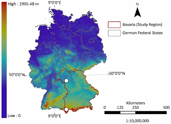
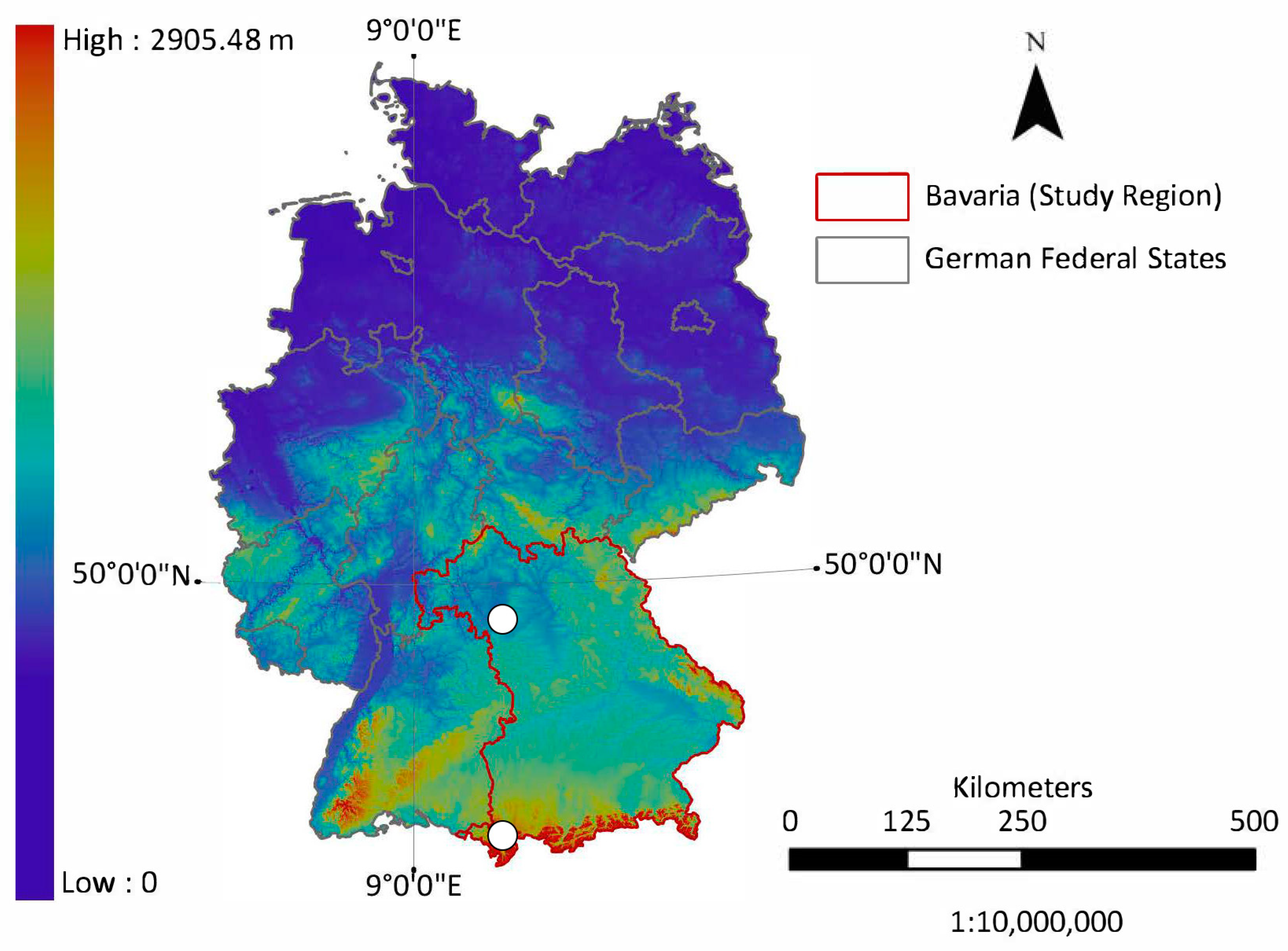
2.1. Experimental Sites

The study sites (presented as white points in Figure 1) are located in the state of Bavaria, Germany. The first site (Triesdorf) is located southwest of Nuremberg in a rural, sparsely populated region of Middle Franconia in northern Bavaria at an elevation of approximately 420 m above sea level on relatively flat lowland terrain. The typical soil type of the region is brown earth, which originated from weathered sand- and claystone [34].

The second site (Kempten) is located in southern Bavaria, east of Lake Constance and close to the Alps. This site is found in the Alpine Foreland at an elevation of around 750 m above sea level on relatively flat terrain of a former river basin in an otherwise hilly region. The typical soil type of the region is brown and para brown earth, which originated from limestone and loamy moraine sediments [34].

The mean temperatures of 2016 were above the long-term average at both test sites (8.9 and 8.6 °C). The total precipitation was significantly below average in Triesdorf (596 mm) and slightly above average in Kempten (1330 mm). The 30-year average (1981–2010) temperatures were 8.3 and 7.6 °C while the average yearly precipitations were 751 and 1261 mm for Triesdorf and Kempten, respectively [35]. According to the Koeppen Geiger climate classification, the climate for the study areas can be classified as a temperate, oceanic type (warm summer, wet winter; Climate zone Cfb).

2.2. Remotely Sensed Data

The dataset that we used consists of 50 Sentinel-1 Ground Range Detected (GRD), Interferometric Wide swath mode (IW) images captured in 2016. Focused Sentinel-1 C-band SAR data was detected, multi-looked and projected to ground range using an Earth ellipsoid model in order to create Level-1 GRD products. The resulting products have approximately square pixel spacing (~10 m in range and azimuth) with reduced speckles. We used the images from acquisition dates every nine days (with some exceptions) from three geometries defined by the Relative Orbit Number (RON) (

Table 1. RONs and their parameters used in this study. The values are given for the study areas.

RON	Asc/Des	AcquisitionTime (UTC)	Average Incidence Angle (degree)
			Triesdorf		Kempten
			Near	Far	Near	Far
66	Des	05:32:45	35.18	35.29	35.22	35.27
117	Asc	17:06:08	37.15	37.26	37.19	37.24
168	Des	05:24:47	36.21	36.32	36.42	36.47

). Figure 2 summarizes the acquisition dates for each geometry.

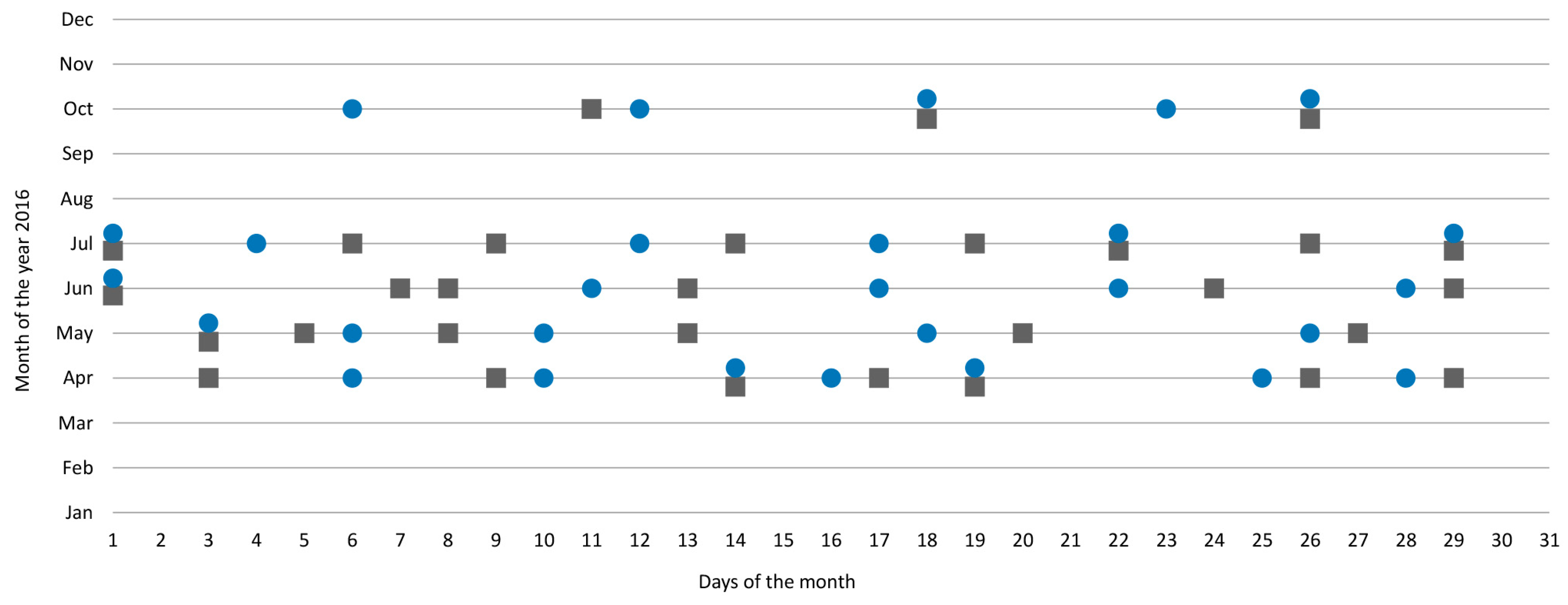
2.3. Ground Truth Campaign

We have used a total of five fields in each of our study sites (Triesdorf and Kempten). The investigated grasslands are intensively used and cut four to five times throughout a season. The typical cutting times were early May, mid of June, late July and October while there was sometimes a fifth cutting in early September. Having been run in parallel to the Sentinel-1 acquisitions, the field surveys of the Bavarian state research center for agriculture (LfL) provided the exact dates of cutting events for each test field (e.g., on 25 August 2017, field one in Kempten is cut), enabling us to determine the cutting status in each image.

3. Methods

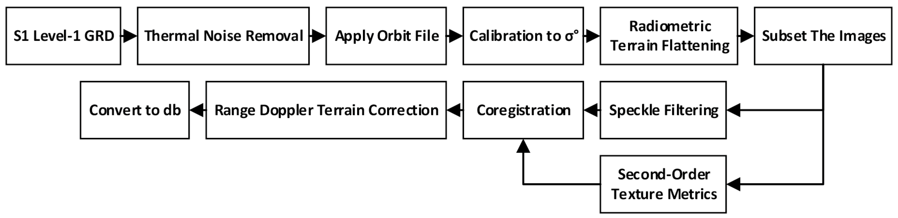
3.1. Data Preprocessing

For preprocessing of SAR data, we used the open source Sentinel-1 toolbox (S1TBX) that is provided by the European Space Agency (ESA). Figure 3 shows a schematic view of the preprocessing flow. Since the proposed model relies on highly accurate radiometric values, we removed thermal noise. To improve the co-registration accuracy, we applied the precise orbit model to each image. This provides information about the geometric location of the SAR images that improves the position accuracy during co-registration. In the next phase, we calibrated all images to the backscatter coefficient. After this, the radiometric terrain flattening using Shuttle Radar Topography Mission (SRTM) 3 sec data and bilinear interpolation was applied to the dataset. For speckle filtering, a 3 × 3 Lee filter was applied and finally, the images were georeferenced using a digital terrain model (Range Doppler Terrain Correction, SRTM) and re-projected to Universal Transverse Mercator (UTM), WGS84. For further analysis, we transformed the corrected intensity data to the logarithmic scale (unit dB).

3.2. ANN Model Description

Artificial Neural Networks (ANNs) are useful in modeling a variety of nonlinear behaviors [36]. ANNs are composed of neurons that are nonlinear computational elements. The neurons establish inverse mapping, which discriminates the relations between inputs and outputs during the training phase. Several studies point out that ANNs are robust in terms of computational speed, stability and accuracy with respect to other investigated algorithms [36,37].

One of the most popular ANNs topologies is the feedforward topology in which each neuron of a layer is connected to all neurons of the successive layer but has no feedback to neurons in the previous layers [38]. In feedforward ANNs, the weighted sum of input datasets is computed with an activation function by each neuron in the network. Equation 1 presents the mathematical representation of ANNs [38]:

$$f_x={\displaystyle \sum }_{j=1}^n{w}_j{d}_j+b_{ }$$

(1)

where d₁, . . . , d_n are inputs; w₁, . . . , w_n are associated connection weights; and b is the bias value. The most commonly used activation function is the sigmoid function. An example of the sigmoid function is the logistic function that is in the range of [0, 1]:

$${\phi }_v= \raisebox{1ex}{$1$}\!\left/ \!\raisebox{-1ex}{$\left(1+e^{-av}\right)$}\right.$$

(2)

where a is the curve steepness for v. The hyperbolic tangent function provides better results than those obtained with the sigmoid function of Equation 2. Therefore, in this study, we used an anti-symmetric form of sigmoid function with the range from −1 to 1 (hyperbolic tangent function) (Equation (3)).

$${\phi }_v= tan{h}_v$$

(3)

Figure 4 provides the backpropagation algorithm for the training of the network, which is very common in remote sensing studies [39,40]. The backpropagation algorithm minimizes the Mean Square Error (MSE) between the multilayered feedforward perception output and the desired output by using a gradient search technique [38].

3.3. Model Implementation

In this study, we used multilayer perceptron neural networks, which are the most suitable topology for information retrieval [38,41]. We have used VV and VH polarization backscattering intensities that are expected to be more suitable for grassland cutting status monitoring compared to HH and HV polarization [42,43]. Therefore, six of the input parameters include VV and VH polarization backscattering intensity for the checking date; VV and VH polarization backscattering intensity for nine days before the checking date; and VV and VH polarization backscattering intensity for eighteen days before the checking date.

Further input variables are the second-order texture metrics (

Table 2. List of input variables used. Gr stands for the distinct grey level numbers.

Name	Acronyms	Formula	Equation Number
VV SAR Intensity	VV-Int	---	---
VH SAR Intensity	VH-Int
VV SAR Homogeneity	VV-Hom	${\displaystyle {\displaystyle \sum }_{i=1}^{Gr}}{\displaystyle {\displaystyle \sum }_{j=1}^{Gr}}\frac{1}{{\left(i-j\right)}^2+1}\ast D{N}_{ij}$	(Equation 5)
VH SAR Homogeneity	VH-Hom
VV SAR Entropy	VV-Ent	${\displaystyle {\displaystyle \sum }_{i=1}^{Gr}}{\displaystyle {\displaystyle \sum }_{j=1}^{Gr}}\log \left(D{N}_{ij}\right)\ast D{N}_{ij}$	(Equation 6)
VH SAR Entropy	VH-Ent
VV SAR Contrast	VV-Con	${\displaystyle {\displaystyle \sum }_{i=1}^{Gr}}{\displaystyle {\displaystyle \sum }_{j=1}^{Gr}}{\left(i-j\right)}^2\ast D{N}_{ij}$	(Equation 7)
VH SAR Contrast	VH-Con
VV SAR Dissimilarity	VV-Dis	${\displaystyle {\displaystyle \sum }_{i=1}^{Gr}}{\displaystyle {\displaystyle \sum }_{j=1}^{Gr}}\left|i-j\right|\ast D{N}_{ij}$	(Equation 8)
VH SAR Dissimilarity	VH-Dis

), including Homogeneity, Entropy, Contrast and Dissimilarity (for the checking date), that are calculated for each polarization (eight parameters in total for both VV and VH channels). Second-order texture metrics show the number of occurrences of the relationship between a pixel and its specified neighboring pixels [44]. We used a 3 × 3 kernel as it is considered to be suitable for computing the texture matrix and extracting enough spatial information to distinguish among different land features [45]. All the input parameters were normalized to a range [−1, 1] using the following equation [40]:

$$D_{new}= 1-\left(\raisebox{1ex}{$2\left(D-D_{min}\right)$}\!\left/ \!\raisebox{-1ex}{$D_{max}- D_{min}$}\right.\right)$$

(4)

where D_new is the normalized value, D_min is the minimum value and D_max is the maximum value in the parameter dataset.

Overall, the dataset consists of 70 samples (checking dates), which were utilized for training/testing and validating the model. We randomly selected 60% and 10% of the data set for training and testing, respectively. The remaining samples (10 and 11 samples for Triesdorf and Kempten, respectively) were used for final model validation. The network training was repeated ten times for each topology. Subsequently, we selected the network with the highest accuracy, which implies that the retained model resides within the best 10% of the distribution of all possible models [46].

The early stopping procedure was used to determine the stop point for the training since it enables the optimization of the generalization properties of the network to avoid overfitting [38]. The early stopping procedure constantly evaluates the performance of the network during the training process. The number of hidden nodes was optimized by trial and error and ranged between 5 and 35 depending on the number of input parameters. The output function of the network returns 0 for a detected cutting and 1 if no cutting occurred. The simulation of the ANNs was conducted with the Stuttgart Neural Network Simulator (SNNS) [47].

4. The Results

In the final step of the model development, we analyzed different topologies by changing the input parameters of the model in order to assess the influence of different sets of inputs on model accuracy. We started by considering only VV and VH parameters for the checking date as the input layer (called “a” in

Table 3. Comparison of results using different input parameter combinations; the model architecture [x–y–z] summarizes the number of input parameters [x], the number of nodes in the hidden layer [y] and the number of output nodes [z].

	(a)	(b)	(c)	(d)
NN model architecture	2–7–1	6–15–1	10–25–1	14–31–1
Overall accuracy [%]	14.28	47.61	80.95	85.71
MSE	5.60	3.20	0.06	0.008

) of the models. After this, we increased the input parameters to six and ten by adding the VV and VH parameters of 9 days and 18 days before the checking dates (called “b” in Table 3) and the homogeneity and entropy parameters (for VV and VH polarizations) for the checking date (called “c” in Table 3), respectively. Finally, we increased the input parameters to fourteen by adding contrast and dissimilarity parameters (for VV and VH polarizations) for the checking date (called “d” in Table 3). For each input set, the topology and calibration with the highest performance in terms of overall accuracy and MSE has been selected and presented in Table 3. Table 3 also highlights the model architecture (no. of input parameters – no. of nodes in the hidden layer – output) of the best models.

Figure 5 exemplarily presents the MSE of the test set “d” as a function of the number of hidden nodes. Considering generalization, time load and accuracy, the network with 31 nodes provided the lowest MSE compared with the other possibilities. In total, approximately 9000 training cycles were sufficient for training the network. The results of the accuracy assessment based on our validation dataset are shown in

Table 4. Confusion matrix and accuracies of the validation set on input set “d”.

		Ground-Truth		Total	User’s Accuracy%
		Cut	Uncut
Predicted	Cut	6	1	7	85.71
	Uncut	2	12	14	85.71
Total		8	13	21
Producer’s Accuracy (%)		75.00	92.30
Overall Accuracy (%)	85.71
Cohen’s Kappa	0.69

.

Cohen’s Kappa for the input set “d” (Table 4) shows that the proposed algorithm achieves acceptable detection results for the validation dataset (with an overall accuracy of 85.71%). For cutting events, the commission and omission errors are 25.00% and 14.29%, respectively. Growing (no cutting) events show a commission error of 7.7% and an omission error of 14.29%.

5. Discussion

The results presented in Table 3 demonstrate that increasing the number of components in the input layer progressively decreased the MSE. We observed a significant improvement when the second-order texture metrics of the checking date were added to the input layer (MSE reduced by 3.14), which indicates that the ANN is able to constructively combine the information of each input node. The best overall accuracy of 85.71% is obtained for the model generated by the input set “d”, which results in an increase of 71.43% in the overall accuracy compared to the best model using VV and VH parameters for the checking date (input set a). The overall accuracies increased by 52.38% and 57.14% when the homogeneity/entropy (input set b) and contrast/dissimilarity parameters (for VV and VH polarizations), respectively, were used along with the other parameters (input set c).

For model evaluation, it is essential to identify the conditions in which the proposed approach generates poor accuracies. The highest commission error (25%) occurred at a cutting event at Triesdorf on October 27th, 2016. For this date, no significant correlation could be established between the backscattering coefficient and the vegetation biomass. Since various factors, i.e., system-dependent (e.g., radar wavelength, mean incidence angle, polarization) and target/weather-dependent (e.g., wind speed, temperature and precipitation) influence the microwave scattering of grassland, it is difficult to isolate a single factor.

Weather clearly affects both structure and water content of grass significantly. For example, Wooding et al. proved that rainfall of about 10 mm prior to SAR acquisition has led to increases of 1–4 dB in the backscattering of grass, bare soil and wheat-bare soil cover types [48] while Wind affects plant microclimates. Temperature changes are important due to the highly differing dielectric properties of ice and liquid water. Moreover, different species associations showed differences in the backscatter response that were partially related to herbage height. Furthermore, these differences were significantly influenced by canopy structure and underlying soil condition and biomass water content [48].

Therefore, we checked the weather data before and during October 27. Since the weather stations in the study site did not record any rainfall or wind speed five days before Sentinel-1 overpass, a direct influence of rainfall or wind can be neglected. The species composition of the test fields is unknown. However, we assume that the species composition does not significantly change between the third/fourth and fifth cut. In spring and early summer, early cutting may positively influence the occurrence of rapidly growing grasses while smaller growing grasses and herbs may be reduced. Therefore, the species composition may be of special interest when analyzing different grassland types.

Furthermore, soil moisture influences the backscattering signal. Schieche et al. proved that the soil water content has little influence on C-Band backscatter in the presence of dense vegetation [25], which may explain why the proposed approach failed to detect a cutting event at Triesdorf on October 27th, 2016. In Germany, the grassland fields that were cut 4–5 times a year show a low amount of biomass in autumn (the field measurements indicate less than 100 grams/sqm) in comparison with the biomass amount in April–May (more than 3.0 kg/sqm of biomass on the study sites). We assume that there are different contributions of soil backscatter in October and late spring/summer [49,50]. Therefore, a sparsely vegetated field with a high amount of soil contributing to the total backscatter probably caused the outlier event on October 27.

We assume that model performance can be improved by adding further input parameters, such as the average incidence angle. A shallow incidence angle data would allow us to retrieve more vegetation signals. Furthermore, the underlying soil is more evident at steeper incidence angles as the SAR pulse travel length through the vegetation layer increases with an increase in the incidence angle. Moreover, Ulaby et al. demonstrated the effect of varying incidence angles on backscattering coefficients along the crop cycle [51]. They mentioned that the difference can reach 0.35 dB⁰⁻¹ in C-band over bare soils and decreases to a value close to zero when the surface is fully vegetated (about 0.05 dB⁰⁻¹). Tamm et al. demonstrated that median VV and VH polarization coherence values were significantly higher after a mowing event [24]. Therefore, the use of interferometric coherence could also be beneficial for increasing the performance of the model.

6. Conclusions

The aim of this study was to demonstrate the capability of multilayer perceptron neural networks as an automated method for grassland cutting status detection. There were four different sets of input parameters, which include (a) VV and VH parameters for the checking date; (b) VV and VH parameters of 9 days and 18 days before the checking dates plus set ‘a’; (c) homogeneity and entropy parameters (for VV and VH polarizations) for the checking date plus set ‘b’; and (d) contrast and dissimilarity parameters (for VV and VH polarizations) for the checking date plus ‘c’. These sets of parameters were used for model development in order to assess the influence of different inputs on model accuracies.

We used four different setups with an increasing number of input parameters (2 to 14, including VV and VH parameters for the checking date as well as 9 days and 18 days before the checking dates, homogeneity, entropy, contrast and dissimilarity).

Twenty-one different models with varying numbers of hidden nodes (for each input set) were separately trained. The network with 14 input parameters and 31 hidden nodes performed best in terms of generalization, time load and accuracy (overall accuracy of 85.71% for the validation dataset). The results demonstrate that the machine learning inversion model is capable of detecting grassland cutting status with a good level of precision. Nevertheless, multilayer perceptron models can be enhanced by a larger and more diverse training/testing dataset.

Concerning polarization as a system-dependent influencing factor, several studies have reported stronger backscatter from grass in VV polarization compared to HH polarization, which interacts more strongly with broad-leaved canopies [52,53]. The geometric and dielectric properties of different grassland types change rapidly over the year, which alters the backscatter signal response. For each acquisition date, the test fields across the study areas are under heterogeneous conditions due to differences in grazing intensity and moisture conditions. As a result, it seems infeasible to determine a single wavelength or polarization that is best suited to detect cutting events.

We suggest that model performance might be further improved by adding different frequencies, angles of observation and polarization as input parameters. However, the presented model demonstrated the general applicability of neural network approaches and SAR data for cutting status detection.

References

1. Ali, I.; Cawkwell, F.; Dwyer, E.; Barrett, B.; Green, S. Satellite remote sensing of grasslands: From observation to management. J. Plant Ecol. 2016, 9, 649–671. [Google Scholar] [CrossRef]
2. O’Mara, F.P. The role of grasslands in food security and climate change. Ann. Bot.-Lond. 2012, 110, 1263–1270. [Google Scholar] [CrossRef] [PubMed] [Green Version]
3. Topfer, K.; Wolfensohn, J.; Lash, J. World Resources 2000–2001: People and Ecosystems: The Fraying Web of Life; World Resources Inst.: Washington, DC, USA, 2000; 389p. [Google Scholar]
4. Scurlock, J.M.O.; Hall, D.O. The global carbon sink: a grassland perspective. Glob. Chang. Biol. 1998, 4, 229–233. [Google Scholar] [CrossRef]
5. Bergman, K.O.; Ask, L.; Askling, J.; Ignell, H.; Wahlman, H.; Milberg, P. Importance of boreal grasslands in Sweden for butterfly diversity and effects of local and landscape habitat factors. Biodivers. Conserv. 2008, 17, 139–153. [Google Scholar] [CrossRef]
6. Pokluda, P.; Hauck, D.; Cizek, L. Importance of marginal habitats for grassland diversity: Fallows and overgrown tall-grass steppe as key habitats of endangered ground-beetle Carabus hungaricus. Insect Conserv. Divers. 2012, 5, 27–36. [Google Scholar] [CrossRef]
7. Voormansik, K.; Jagdhuber, T.; Olesk, A.; Hajnsek, I.; Papathanassiou, K.P. Towards a detection of grassland cutting practices with dual polarimetric TerraSAR-X data. Int. J. Remote Sens. 2013, 34, 8081–8103. [Google Scholar] [CrossRef]
8. Herrmann, A.; Kelm, M.; Kornher, A.; Taube, F. Performance of grassland under different cutting regimes as affected by sward composition, nitrogen input, soil conditions and weather—A simulation study. Eur. J. Agron. 2005, 22, 141–158. [Google Scholar] [CrossRef]
9. Lopes, M.; Fauvel, M.; Girard, S.; Sheeren, D. Object-Based Classification of Grasslands from High Resolution Satellite Image Time Series Using Gaussian Mean Map Kernels. Remote Sens. (Basel) 2017, 9. [Google Scholar] [CrossRef]
10. Newton, A.C.; Hill, R.A.; Echeverria, C.; Golicher, D.; Benayas, J.M.R.; Cayuela, L.; Hinsley, S.A. Remote sensing and the future of landscape ecology. Prog. Phys. Geogr. 2009, 33, 528–546. [Google Scholar] [CrossRef] [Green Version]
11. Dusseux, P.; Corpetti, T.; Hubert-Moy, L.; Corgne, S. Combined Use of Multi-Temporal Optical and Radar Satellite Images for Grassland Monitoring. Remote Sens. (Basel) 2014, 6, 6163–6182. [Google Scholar] [CrossRef] [Green Version]
12. Hong, G.; Zhang, A.N.; Zhou, F.Q.; Brisco, B. Integration of optical and synthetic aperture radar (SAR) images to differentiate grassland and alfalfa in Prairie area. Int. J. Appl. Earth Obs. 2014, 28, 12–19. [Google Scholar] [CrossRef]
13. Friedl, M.A.; Schimel, D.S.; Michaelsen, J.; Davis, F.W.; Walker, H. Estimating grassland biomass and leaf area index using ground and satellite data. Int. J. Remote Sens. 1994, 15, 1401–1420. [Google Scholar] [CrossRef]
14. Skriver, H.; Svendsen, M.T.; Thomsen, A.G. Multitemporal C- and L-band polarimetric signatures of crops. IEEE Trans. Geosci. Remote Sens. 1999, 37, 2413–2429. [Google Scholar] [CrossRef]
15. Kasischke, E.S.; Melack, J.M.; Dobson, M.C. The use of imaging radars for ecological applications—A review. Remote Sens. Environ. 1997, 59, 141–156. [Google Scholar] [CrossRef]
16. Schuster, C.; Schmidt, T.; Conrad, C.; Kleinschmit, B.; Forster, M. Grassland habitat mapping by intra-annual time series analysis—Comparison of RapidEye and TerraSAR-X satellite data. Int. J. Appl. Earth Obs. 2015, 34, 25–34. [Google Scholar] [CrossRef]
17. Wiseman, G.; McNairn, H.; Homayouni, S.; Shang, J.L. RADARSAT-2 Polarimetric SAR Response to Crop Biomass for Agricultural Production Monitoring. IEEE J.-STARS 2014, 7, 4461–4471. [Google Scholar] [CrossRef]
18. Barrett, B.; Nitze, I.; Green, S.; Cawkwell, F. Assessment of multi-temporal, multi-sensor radar and ancillary spatial data for grasslands monitoring in Ireland using machine learning approaches. Remote Sens. Environ. 2014, 152, 109–124. [Google Scholar] [CrossRef] [Green Version]
19. Stiles, J.M.; Sarabandi, K. Electromagnetic scattering from grassland Part I: A fully phase-coherent scattering model. IEEE Trans. Geosci. Remote Sens. 2000, 38, 339–348. [Google Scholar] [CrossRef]
20. Oh, Y.; Sarabandi, K.; Ulaby, F.T. An Empirical-Model and an Inversion Technique for Radar Scattering from Bare Soil Surfaces. IEEE Trans. Geosci. Remote Sens. 1992, 30, 370–381. [Google Scholar] [CrossRef]
21. Luckman, A.J. The effects of topography on mechanisms of radar backscatter from coniferous forest and upland pasture. IEEE Trans. Geosci. Remote Sens. 1998, 36, 1830–1834. [Google Scholar] [CrossRef]
22. Hill, M.J.; Ticehurst, C.J.; Lee, J.S.; Grunes, M.R.; Donald, G.E.; Henry, D. Integration of optical and radar classifications for mapping pasture type in western Australia. IEEE Trans. Geosci. Remote Sens. 2005, 43, 1665–1681. [Google Scholar] [CrossRef]
23. Hill, M.J.; Donald, G.E.; Vickery, P.J. Relating radar backscatter to biophysical properties of temperate perennial grassland. Remote Sens. Environ. 1999, 67, 15–31. [Google Scholar] [CrossRef]
24. Tamm, T.; Zalite, K.; Voormansik, K.; Talgre, L. Relating Sentinel-1 Interferometric Coherence to Mowing Events on Grasslands. Remote Sens. 2016, 8, 802. [Google Scholar] [CrossRef]
25. Schieche, B.; Erasmi, S.; Schrage, T.; Hurlemann, P. Monitoring and registering of grassland and fallow fields with multitemporal ERS data within a district of lower Saxony, Germany. In Proceedings of the IEEE 1999 International Geoscience and Remote Sensing Symposium, IGARSS’99 Proceedings, Hamburg, Germany, 28 June–2 July 1999; Volume 752, pp. 759–761. [Google Scholar]
26. Smith, A.M.; Buckley, J.R. Investigating RADARSAT-2 as a tool for monitoring grassland in western Canada. Can. J. Remote Sens. 2011, 37, 93–102. [Google Scholar] [CrossRef]
27. Moreau, S.; Le Toan, T. Biomass quantification of Andean wetland forages using ERS satellite SAR data for optimizing livestock management. Remote Sens. Environ. 2003, 84, 477–492. [Google Scholar] [CrossRef]
28. Macelloni, G.; Paloscia, S.; Pampaloni, P.; Marliani, F.; Gai, M. The relationship between the backscattering coefficient and the biomass of narrow and broad leaf crops. IEEE Trans. Geosci. Remote Sens. 2001, 39, 873–884. [Google Scholar] [CrossRef]
29. Schuster, C.; Ali, I.; Lohmann, P.; Frick, A.; Förster, M.; Kleinschmit, B. Towards Detecting Swath Events in TerraSAR-X Time Series to Establish NATURA 2000 Grassland Habitat Swath Management as Monitoring Parameter. Remote Sens. 2011, 3, 1308–1322. [Google Scholar] [CrossRef] [Green Version]
30. Voormansik, K.; Jagdhuber, T.; Zalite, K.; Noorma, M.; Hajnsek, I. Observations of Cutting Practices in Agricultural Grasslands Using Polarimetric SAR. IEEE J.-STARS 2016, 9, 1382–1396. [Google Scholar] [CrossRef]
31. Yuan, Z.; Wang, L.N.; Ji, X. Prediction of concrete compressive strength: Research on hybrid models genetic based algorithms and ANFIS. Adv. Eng. Softw. 2014, 67, 156–163. [Google Scholar] [CrossRef]
32. Clevers, J.G.P.W.; van der Heijden, G.W.A.M.; Verzakov, S.; Schaepman, M.E. Estimating grassland Biomass using SVM band shaving of hyperspectral data. Photogramm. Eng. Remote Sens. 2007, 73, 1141–1148. [Google Scholar] [CrossRef]
33. Ali, I.; Cawkwell, F.; Dwyer, E.; Green, S. Modeling Managed Grassland Biomass Estimation by Using Multitemporal Remote Sensing Data—A Machine Learning Approach. IEEE J.-STARS 2017, 10, 3254–3264. [Google Scholar] [CrossRef]
34. BGR. BÜK2000. Available online: https://www.bgr.bund.de/DE/Themen/Boden/Informationsgrundlagen/Bodenkundliche_Karten_Datenbanken/BUEK200/buek200_node.html (accessed on 15 January 2018).
35. DWD. Available online: http://www.dwd.de/DE/leistungen/klimadatendeutschland/mittelwerte/nieder_8110_akt_html.html?view=nasPublication&nn=16102 (accessed on 15 January 2018).
36. Atkinson, P.M.; Tatnall, A.R.L. Neural networks in remote sensing—Introduction. Int. J. Remote Sens. 1997, 18, 699–709. [Google Scholar] [CrossRef]
37. Taravat, A.; Latini, D.; Frate, F.D. Fully Automatic Dark-Spot Detection From SAR Imagery With the Combination of Nonadaptive Weibull Multiplicative Model and Pulse-Coupled Neural Networks. IEEE Trans. Geosci. Remote Sens. 2014, 52, 2427–2435. [Google Scholar] [CrossRef]
38. Bishop, C.M. Neural Networks for Pattern Recognition; Oxford University Press: Oxford, UK, 1995. [Google Scholar]
39. Foody, G.M. Thematic map comparison: Evaluating the statistical significance of differences in classification accuracy. Photogramm. Eng. Remote Sens. 2004, 70, 627–633. [Google Scholar] [CrossRef]
40. Skidmore, A.K.; Turner, B.J.; Brinkhof, W.; Knowles, E. Performance of a neural network: Mapping forests using GIS and remotely sensed data. Photogramm. Eng. Remote Sens. 1997, 63, 501–514. [Google Scholar]
41. Taravat, A.; Proud, S.; Peronaci, S.; Del Frate, F.; Oppelt, N. Multilayer Perceptron Neural Networks Model for Meteosat Second Generation SEVIRI Daytime Cloud Masking. Remote Sens. (Basel) 2015, 7, 1529–1539. [Google Scholar] [CrossRef] [Green Version]
42. McNairn, H.; Champagne, C.; Shang, J.; Holmstrom, D.; Reichert, G. Integration of optical and Synthetic Aperture Radar (SAR) imagery for delivering operational annual crop inventories. ISPRS J. Photogramm. Remote Sens. 2009, 64, 434–449. [Google Scholar] [CrossRef]
43. McNairn, H.; Shang, J.; Champagne, C.; Jiao, X. TerraSAR-X and RADARSAT-2 for crop classification and acreage estimation. In Proceedings of the 2009 IEEE International Geoscience and Remote Sensing Symposium, Cape Town, South Africa, 12–17 July 2009; pp. II-898–II-901. [Google Scholar]
44. Haralick, R.M.; Shanmugam, K.; Dinstein, I. Textural Features for Image Classification. IEEE Trans. Syst. Man Cybern. 1973, SMC3, 610–621. [Google Scholar] [CrossRef]
45. Su, W.; Li, J.; Chen, Y.; Liu, Z.; Zhang, J.; Low, T.M.; Suppiah, I.; Hashim, S.A.M. Textural and local spatial statistics for the object-oriented classification of urban areas using high resolution imagery. Int. J. Remote Sens. 2008, 29, 3105–3117. [Google Scholar] [CrossRef]
46. Taravat, A.; Del Frate, F.; Cornaro, C.; Vergari, S. Neural Networks and Support Vector Machine Algorithms for Automatic Cloud Classification of Whole-Sky Ground-Based Images. IEEE Geosci. Remote Sens. 2015, 12, 666–670. [Google Scholar] [CrossRef]
47. Zell, A.; Mamier, G.; Vogt, M.; Mache, N.; Hübner, R.; Döring, S.; Herrmann, K.; Soyez, T.; Schmalzl, M.; Sommer, T. SNNS, Stuttgart Neural Network Simulator, User Manual; Version 4.1; Institute for Parallel and Distributed High Performance Systems, University of Stuttgart: Stuttgart, Germany, 1995. [Google Scholar]
48. Wooding, M.; Griffiths, G.; Evans, R.; Bird, P.; Kenward, D.; Keyte, G.E. Temporal monitoring of soil moisture using ERS-1 SAR data. Available online: https://bit.ly/2OnQyFr (accessed on 25 March 2019).
49. Zoughi, R.; Bredow, J.; Moore, R.K. Evaluation and Comparison of Dominant Backscattering Sources at 10 Ghz in 2 Treatments of Tall-Grass Prairie. Remote Sens. Environ. 1987, 22, 395–412. [Google Scholar] [CrossRef]
50. Ulaby, F.T.; Long, D.G.; Blackwell, W.J.; Elachi, C.; Fung, A.K.; Ruf, C.; Sarabandi, K.; Zebker, H.A.; Van Zyl, J. Microwave Radar and Radiometric Remote Sensing; University of Michigan Press: Ann Arbor, MI, USA, 2014. [Google Scholar]
51. Ulaby, F.T.; Batlivala, P.P.; Dobson, M.C. Microwave Backscatter Dependence on Surface Roughness, Soil Moisture and Soil Texture: Part I-Bare Soil. IEEE Trans. Geosci. Electron. 1978, 16, 286–295. [Google Scholar] [CrossRef]
52. Ferrazzoli, P.; Paloscia, S.; Pampaloni, P.; Schiavon, G.; Sigismondi, S.; Solimini, D. The potential of multifrequency polarimetric SAR in assessing agricultural and arboreous biomass. IEEE Trans. Geosci. Remote Sens. 1997, 35, 5–17. [Google Scholar] [CrossRef]
53. Pierce, L.E.; Bergen, K.M.; Dobson, M.C.; Ulaby, F.T. Multitemporal land-cover classification using SIR-C/X-SAR imagery. Remote Sens. Environ. 1998, 64, 20–33. [Google Scholar] [CrossRef]
Figure 1. Map of Germany with locations of in-situ study areas highlighted in white. The colors represent relief elevation.
Remotesensing 11 00711 g001
Figure 2. Sentinel-1 acquisitions used in the study. The squares and circles represent Triesdorf and Kempten sites, respectively.
Remotesensing 11 00711 g002
Figure 3. Schematic view of the Sentinel-1 pre-processing workflow.
Remotesensing 11 00711 g003
Figure 4. The backpropagation ANN model used in this study. The input layer (d) is connected to a layer of hidden nodes (n), which are in turn connected to the output layer (x).
Remotesensing 11 00711 g004
Figure 5. Training MSE as a function of the number of hidden nodes for input set “d”.
Remotesensing 11 00711 g005