Preliminary Assessment of Turbidity and Chlorophyll Impact on Bathymetry Derived from Sentinel-2A and Sentinel-3A Satellites in South Florida

Abstract

Evaluation of the impact of turbidity on satellite-derived bathymetry (SDB) is a crucial step for selecting optimal scenes and for addressing the limitations of SDB. This study examines the relatively high-resolution MultiSpectral instrument (MSI) onboard Sentinel-2A (10–20–60 m) and the moderate-resolution Ocean and Land Color instrument (OLCI) onboard Sentinel-3A (300 m) for generating bathymetric maps through a conventional ratio transform model in environments with some turbidity in South Florida. Both sensors incorporate additional spectral bands in the red-edge near infrared (NIR) region, allowing turbidity detection in optically shallow waters. The ratio model only requires two calibration parameters for vertical referencing using available chart data, whereas independent lidar surveys are used for validation and error analysis. The MSI retrieves bathymetry at 10 m with errors of 0.58 m at depths ranging between 0–18 m (limit of lidar survey) in West Palm Beach and of 0.22 m at depths ranging between 0–5 m in Key West, in conditions with low turbidity. In addition, this research presents an assessment of the SDB depth limit caused by turbidity as determined with the reflectance of the red-edge bands at 709 nm (OLCI) and 704 nm (MSI) and a standard ocean color chlorophyll concentration. OLCI and MSI results are comparable, indicating the potential of the two optical missions as interchangeable sensors that can help determine the selection of the optimal scenes for SDB mapping. OLCI can provide temporal data to identify water quality characteristics and general SDB patterns. The relationship of turbidity with depth detection may help to enhance the operational use of SDB over environments with varying water transparency conditions, particularly in remote and inaccessible regions of the world.

1. Introduction

Updated and accurate coastal bathymetry is becoming a crucial source of information required for a wide range of purposes, including navigation, resource exploitation, fisheries, aquaculture, coastal management, spatial planning, benthic research, and tourism. According to International Hydrographic Office (IHO) publication, an estimated 70% of the world’s littoral zone is not mapped to modern standards [1,2]. One reason for this limited coastal coverage is that traditional survey methods for mapping water depth are extremely expensive. Knowledge of ocean bathymetry has progressed rapidly in this century because of the advancement in techniques using acoustics and optics [3]. Since the first studies in late 1970s, remote sensing of bathymetry has taken several forms, each having its own detection depth, accuracy, strengths, limitations, and best application settings [4,5].

When using satellite imagery, different approaches have been applied to characterize satellite-derived bathymetry (SDB) from the physics of light in the water. These include semi-analytical equations [6,7] and approximation equations [8] with empirically tuned coefficients. Other approaches use optimization to solve for the coefficients from semi-analytical [9,10] or analytical [5,11] models. The analytical models can be utilized to solve simultaneously for depth, benthic albedo, cover, and water optical properties, but they are more complex to implement, as they require the parameterization of reflectance spectra of the major benthic habitats, basic information about water optical properties, and extremely accurate atmospheric correction. Current atmospheric correction methods, while generally effective, do not consistently produce the sufficiently accurate water reflectance needed by analytical models [11], which makes these models less efficient from an operational or recursive monitoring point of view. Generally, about 90% of sensor-measured radiance over water bodies results from atmospheric effects, so it is critical to implement an accurate atmospheric correction in order to retrieve minimal errors in water reflectance, especially in coastal and other optically complex waters [12,13]. The approximation equations require that imagery be pre-processed to physical units of water reflectance, but they can tolerate some residual error [8]. Also, when multi-temporal approaches are used, the retrieved water reflectances need to be consistent, even with different atmospheric conditions [8,14].

Despite the fact that total water reflectance is primarily related to water depth and bottom type in optically shallow areas, and secondarily to water transparency, water clarity still has significant and varying impacts on the accuracy of SDB [15]. In fact, water turbidity is the most significant factor altering SDB precision by limiting light penetration through the water [4]. Suspended particulate matter, a main contributor to turbidity, interferes with the ray-path geometry of light. As a result, turbidity plumes are identified as bottom in SDB calculations, creating false shoals and reducing drastically the sensible depth [16]. Additionally, waters of different turbidity levels scatter the incoming radiation differently, introducing further complexity in highly dynamic coastal regions. There have been a few studies that have developed different methodologies to map water depths accounting for the turbidity signal to some extent [16,17,18,19,20,21]. An analytical retrieval method from hyperspectral data is one example, which compensates for the degradation of accuracy in depth retrievals as the waters become deeper or more turbid [22]. Regardless of the technique, turbidity is the most challenging constraint to the routine application of SDB worldwide [2,4]. Taking into account that passive satellite imagery might be the only robust, cheap and synoptic technique for routine bathymetric mapping of nearshore environments worldwide, further research should be conducted to understand the limitations of turbidity and its impact on SDB.

The motivation of this research was to evaluate and quantify the influence of moderate turbidity on SDB in environments that have spatial and temporal variability in water transparency. In regions of the world where in situ water clarity measurements are not feasible, satellite imagery can be an effective approach for estimating turbidity. This research looks at the two optical missions of the Sentinel Constellation within the Copernicus program: the multispectral instrument (MSI) onboard Sentinel-2A and the ocean and land color instrument (OLCI) onboard Sentinel-3A. While the MSI was intended for global monitoring of land, it has already led to investigation of nearshore and inland water parameters [23,24,25,26]. Given its higher spatial resolution (10 m) compared to Landsat (30 m) and other routine global monitoring sensors, MSI should be considered as a key bathymetric mapping satellite. OLCI data, at 300 m, can provide only a reconnaissance SDB. However, its two-day repeat (daily with Sentinel-3B operational) provides a high frequency surrogate for rapid assessment of MSI product stability after atmospheric correction and for temporal analysis of SDB model performance over variable water clarity conditions. Both Sentinel-2 and Sentinel-3 missions have three spectral bands within the “red-edge” (700–780 nm) of the near infrared (NIR) region, enabling further insights into water quality examination over optically complex coastal/inland waters [12,13,25,27]. Recent studies have confirmed MSI radiometric performances are comparable to those of the Lansdat-8 operational land imager (OLI), highlighting that high-quality products can be derived from Sentinel-2 [28,29]. In addition, some works have already demonstrated the feasibility of Sentinel-2 to map bottom depth [30,31,32,33].

The urgent requirement of accurate bathymetry has been highlighted in the “Copernicus for Coastal Zone Monitoring and Management workshop”, where many end users asked for up-to-date, high-resolution bathymetric information for improvement of coastal zone monitoring services, specifically mapping shallow waters [34]. In this sense, the Sentinel-2/3 missions represent a new perspective for remotely sensed seabed topography extraction with the advantages of a fast, flexible, and economic solution. As such, Sentinel optical data have become a topic of increased interest for coastal monitoring worldwide, with a demand to determine strategies for implementing SDB within operational production processes [35]. One method for estimating depth in clear water uses a ratio transform approximation to describe the changing light with depth [8]. This model, which solves the vertical tuning empirically, was designed to support routine mapping in areas with extremely limited low-resolution calibration data. Many studies have demonstrated the great potential of this model for bathymetric retrieval in several regions worldwide [36,37,38]. A comparison of the band ratio and optimization approaches in Australia showed that these methods yielded similar estimates overall, and both were subject to the same depth limitations mainly associated with the site water characteristics [39]. In this study, we sought to investigate the behavior of this spectrally based bathymetric technique over two moderately turbid regions in United States of interest to the National Atmospheric and Oceanic Administration (NOAA).

2. Materials and Methods

2.1. Study Region

Two sites in South Florida were investigated (Figure 1): Key West and West Palm Beach (or West Palm). These study regions were suitable for method development and testing. Both sites had updated airborne lidar bathymetry data for final validation and error analysis, and waters in these study sites had variably low to moderate turbidity levels [40]. Key West is an island in the Straits of Florida, at the southernmost tip of the limestone archipelago of the Florida Keys. Gradients in water quality have been identified according to distance from shore, with offshore waters being the clearest and most oligotrophic [41,42]. The generally shallow depth of the water column (0 to 6 m) presents the potential for frequent resuspension of the sediments. The basin has mostly carbonate sediments, hard bottoms, coral patches, and benthic vegetation, all of which affect the nature and concentration of suspended solids in the water column [43]. West Palm is a National Historic Landmark located on the Palm Beach barrier island, in southeast Florida. The study area corresponded to a coastal strip in central eastern Palm Beach County. The geomorphology of this area consists of a wide range of bottom types that included coral reefs, hard rounds (rock reefs), and sedimentary features including bar and trough systems as well as sandy bottom types [44,45].

2.2. Satellite Data: Sentinel-2 and Sentinel-3 Missions

The European Space Agency (ESA) developed the Sentinel fleet to meet the operational needs of the European Commission’s Copernicus program. Each Sentinel mission is based on a constellation of two satellites to fulfill revisit and coverage requirements, providing robust data sets for Earth Observation services. These missions carry a range of technologies, such as radar and multi-spectral imaging instruments for land, ocean, and atmospheric monitoring. In this study, both Sentinel-2 and Sentinel-3 satellites were used.

The Sentinel-3 OLCI is a 21-band multispectral sensor. The main characteristics of OLCI include the nominal resolution of 300 m at nadir, 14-bit radiometric resolution (analog to digital), enhanced long-term radiometric stability, and temporal coverage of <3 days at equator with one satellite (ignoring the effect of clouds) [46]. Sentinel-3A was launched on 16 February 2016 and Sentinel-3B was launched on 25 April 2017. Standard OLCI Level-1B imagery was archived at the ESA Science Data Hub (https://scihub.copernicus.eu/). Sentinel-3 data sets were processed using the NOAA satellite automated system, which incorporated the National Aeronautics and Space Administration (NASA) standard ocean color satellite processing software distributed within the Sea-viewing Wide Field-of-view Sensor (SeaWiFS) Data Analysis System (SeaDAS) package (version 7.4) to obtain remote sensing reflectance, hereinafter referred as Rrs (1/sr), in all visible and NIR bands. OLCI processing included surface reflectance correction, specifically corrections for sunglint, whitecaps, and specular reflection. In addition, the SeaDAS OC4 chlorophyll-a (chlor_a, mg/m³) product was also generated using the algorithm defaults [47]. OC4 is a fourth-order polynomial model developed from an empirical relationship of in situ chlorophyll-a to the blue-green Rrs bands using the NASA bio-optical marine algorithm data set [48]. Products were mapped to UTM zone 17 WGS84 ellipsoid at 300 m pixel resolution. OLCI images (n = 177) in South Florida from 1 January 2017 to 31 August 2017 were selected for analysis, using every available scene after atmospheric correction.

Table 1. Sentinel-3A Ocean and Land Color instrument (OLCI) and Sentinel-2A multispectral imager (MSI) spectral band settings used in this study indicating central wavelength, width, and spatial resolution. The associated signal to noise ratio (SNR) at reference radiance for MSI [56] and OLCI [46].

Sentinel-2A (MSI)			Sentinel-3A (OLCI)
Central Wavelength (nm)	Spatial Resolution (m)	Bandwidth (nm)	Central Wavelength (nm)	Spatial Resolution (m)	Bandwidth (nm)
445	60	20	443	300	10
490	10	65	490	300	10
560	10	35	560	300	10
664	10	30	665	300	10
704	20	15	709	300	10
740	20	15	754	300	7.5
783	20	20	779	300	15
865	20	20	865	300	20

presents detailed information of the OLCI spatial and spectral band settings used in this study.

The full Sentinel-2 mission comprises twin polar-orbiting satellites in the same orbit, phased at 180° to each other. Sentinel-2A was launched on 23 June 2015 and Sentinel-2B followed on 7 March 2017. The radiometric resolution of MSI is 12-bit, and spectral and spatial characteristics of the bands used in this study are shown in Table 1. Sentinel-2A scenes for the study areas were downloaded from the Sentinel’s Scientific Data Hub. These images corresponded to Level-1C (L1C) products processed by the payload data ground segment (PDGS), which means data were radiometrically and geometrically corrected top of atmosphere (TOA) products [49]. The calibrated TOA reflectance products are provided to the science/user community at their native spatial resolution in 100 km × 100 km tile formats [49]. In this study, the images of zone 17 in Key West (sub-tile RMH) and West Palm (sub-tile RNK) were used. Only scenes with low cloud coverage and sunglint effects over the study region were selected for further analysis. Since the first MSI image at these locations was released in 2015, only a limited number of partially cloud free data was available because of the poor weather conditions, especially in West Palm. In addition, the acquisition of Sentinel-2A imagery over these regions was lower than a 10-day revisit cycle during several periods. As a result, from December 2015 to May 2017, 14 images were suitable over Key West and 4 images over West Palm (see

Table 2. Details for the processed Sentinel-2A images in Key West (1–14) and West Palm Beach (15–18).

Number Image	Date Acquisition	Sensing Time (GMT)	Tile	Cloud Coverage (%)
1	20151216	16:19	T17RMH	0
2	20160214	16:11	T17RMH	0.15
3	20160822	16:13	T17RMH	1.69
4	20161001	16:04	T17RMH	9.39
5	20161021	16:13	T17RMH	0
6	20161110	16:08	T17RMH	0.61
7	20161120	16:13	T17RMH	0.33
8	20161130	16:13	T17RMH	26.18
9	20161220	16:06	T17RMH	1.04
10	20161230	16:12	T17RMH	0.56
11	20170208	16:12	T17RMH	0.28
12	20170419	16:13	T17RMH	24.9
13	20170509	16:13	T17RMH	15.9
14	20170529	16:13	T17RMH	21.63
15	20160302	15:56	T17RNK	9.95
16	20161127	16:05	T17RNK	0.56
17	20161207	16:05	T17RNK	7.1
18	20170106	16:00	T17RNK	0

for detailed information on Sentinel-2A scenes used in this study). No images were examined after Hurricane Irma (September 2017) since intense resuspension and currents may have modified shallow seabed morphology, confounding comparison with the lidar survey.

Sentinel-2A images were processed to Level-2A (L2A) with the ACOLITE processor developed by the Royal Belgian Institute of Natural Sciences (RBINS), which supports free processing, specifically for aquatic applications, of both Landsat-8 and Sentinel-2 [25,27,50,51]. ACOLITE processing is an image-based approach, and therefore, all input information needed for the atmospheric correction is derived from the image itself, without requiring in situ data. Given the conditions of moderate turbidity in the areas under investigation, a combination of the NIR and short wave infrared (SWIR) channels was used in ACOLITE to return Rrs (1/sr) resampled to 10 m pixel size. We selected the NIR/SWIR (865/1600 nm) bands for the aerosol correction with a user defined epsilon value (maritime aerosol = 1) recommended in low to moderate turbidity waters. This strategy has been shown to improve the quality of the products by minimizing the influence of NIR/SWIR instrument noise [29]. ACOLITE outputs showed some speckle noise, so a spatial filter (median filter 3 × 3 pixel) was applied to each band in order to remove this noise. While not a concern for this study, a 3 × 3 filter will clip features smaller than 4 pixels in area. However, unlike averaging filters, the median filter preserves edges (like channels) without smoothing [52]. Recent studies have showed that the noise reduction of a median filter improves the accuracy of the bathymetry estimates against high-resolution lidar, in contrast to methods (like average filters) that smooth the data [11,14].

Determining turbidity in optically shallow water requires the use of spectral bands that are both sensitive to turbidity and have limited depth penetration in order to avoid substantial interference from the bottom. Red bands were useful for turbidity in South Florida, and can have a strong bottom signal in clear waters as deep as 5 m [53,54]. The absorption by water increases rapidly from red to the “red edge” NIR (700–780 nm). This absorption limits the light received from the bottom, while still returning light scattered from materials in the water. Several studies have already indicated these spectral bands are appropriate for turbidity or suspended solids monitoring in optically shallow regions [12,13,23,24,25]. A recent study has confirmed that Sentinel-2 red-edge bands achieved good accuracies when compared with suspended solid concentrations [55]. In this sense, the red-edge NIR bands have sufficient water absorption to be a good compromise between detecting turbidity and limited detection of the bottom. The 709 and 704 nm bands, with coefficients of water absorption (aw) about 1/3 of 740–783 nm bands, are about three-fold more sensitive to turbidity than the longer bands (see

Table 3. Maximum proportion of incident light (max light) returned from different depths (z = 1, 2, 3, and 4 m) for a carbonate sand bottom (albedo = 50%). The coefficients of water absorption (aw, 1/m) obtained from NASA (https://oceancolor.gsfc.nasa.gov/docs/rsr/rsr_tables/) were used for the different wavelengths in the red-edge spectrum (Table 1) for both the OLCI and the MSI.

Band (nm)	aw (1/m)	Max Light Return 1 m	Max Light Return 2 m	Max Light Return 3 m	Max Light Return 4 m
704	0.687	0.1265	0.032	0.0081	0.0021
709	0.7962	0.102	0.0207	0.0042	0.00085
740	2.768	0.0020	7.810–6	3.110–8	1.210–10
754	2.8666	0.0016	5.310–6	1.710–8	5.510–11
779	2.7101	0.0022	9.810–6	4.410–8	1.910–10
783	2.632	0.0026	1.410–5	6.910–8	3.610–10

). However, they would begin to confuse turbidity with bottom in waters shallower than 2 m. Water at these red-edge wavelengths absorbs much less light than at wavelengths >800 nm [12,13], allowing detection of low to moderate turbidity, so they should be the most useful in relatively clear waters (Table 3). In this study, we used the red-edge bands 709 nm and 704 nm of OLCI and MSI, respectively, as a proxy for turbidity and excluded depths <2 m from turbidity analysis.

2.3. Airborne Lidar Bathymetry and Electronic Navigational Charts

NOAA’s National Geodetic Survey (NGS) collected airborne lidar bathymetry (hereinafter ALB) for Key West in April 2016 and for West Palm Beach in February 2017. These point cloud data sets were both collected using the Riegl VQ-880-G sensor, which provided high-resolution bathymetry in nearshore waters. The Riegl VQ-880-G used a green laser that operated in a circular scan pattern, which could penetrate shallow, clear water to the seafloor. The high-density point data were combined with GPS and other positional data to create precise 3D topobathy elevation models. NGS used coastal elevation data to map the mean high-water shoreline, which is considered the nation’s official shoreline. These high-resolution observations were selected as the reference data set in the two study sites for comparison with the SDB products. The minimum/maximum and mean lidar depths in each study site were 0/8.9 m and 3.91 m for Key West and 0/17.92 m and 8.24 m for West Palm. The data were in UTM zone 17 coordinates and ellipsoid elevations in meters with the NAD83 datum. The vertical accuracy of the surveys was 7.5 cm, collected to meet vertical error at 1 standard deviation, while the horizontal accuracy was 50 cm, collected to meet horizontal accuracy at 1 standard deviation. NOAA uses mean lower low water (MLLW) as chart datum. MLLW is the average height of the lowest tide recorded at a tide station each day during a 19-year recording period, known as the National Tidal Datum Epoch. VDatum was used to convert between NAD83 ellipsoidal heights used for ALB and MLLW. VDatum reported a 9.43 cm uncertainty associated with the transformation. ALB data referenced to the MLLW in both regions were gridded at the MSI’s and OLCI’s image resolutions (10 m and 300 m, respectively) via arithmetic averaging. Arithmetic averaging smooths out the variability of the seabed. The averaging would remove sub-satellite pixel variability that would be detected in the lidar, primarily small channels and bottoms with high rugosity; however, the averaging also excludes this variability from appearing as error in the accuracy assessment.

2.4. Satellite-Derived Bathymetry Estimation

In this study, the model selected was the ratio of log-transformed bands having different absorptions [8]. Because of the exponential change in light with depth, this approach created a linear relationship with depth in waters that were optically shallow in both bands (Equation (1)). The model used the reflectance (Rrs) of each satellite image corrected for atmospheric effects. Since both Sentinel-2 and Sentinel-3 have two similar blue bands (Table 1), the model was tested using coastal blue (hereinafter 445 or 443 nm, for MSI and OLCI, respectively) and blue (hereinafter 490 nm) as the numerator. For MSI, the 445 nm (60 m) blue may be considered for bathymetry because of the high SNR. We included it in some analysis for this reason, although we do not recommend it for mapping because of the severe loss in spatial resolution compared to the 10 m (490 nm) band. We used the ratio of 445 nm or 490 nm (${\lambda }_i$) to 560 nm (${\lambda }_j$) bands (hereinafter SDBgreen), and the ratio of 445 nm or 490 nm (${\lambda }_i$) to 664 nm (${\lambda }_j$) bands (hereinafter SDBred) and determined depths as:

$$\mathrm{SDB}=m_1\mathrm{pSDB}-m_0$$

(1)

where pSDB = $\frac{\ln \left(\mathrm{n}\mathrm{Pi}\mathrm{Rrs}\left({\lambda }_i\right)\right)}{\ln \left(\mathrm{n}\mathrm{Pi}\mathrm{Rrs}\left({\lambda }_j\right)\right)}$.

pSDB is the relative or “pseudo” depth from satellite (dimensionless), SDB is the satellite-derived depth (meters), Rrs is the remote sensing reflectance, m₁ and m₀ are tunable constants to linearly transform (slope and intercept, respectively) the model results to the actual depth in a chart, and n = 1000 is a fixed constant for all areas to assure that both logarithms will be positive under any condition, and that the ratio will produce a linear response with depth [8].

After calculating pSDB, the parameters m₁ and m₀ were tuned by linear regression against reference depth data. As this model had only two coefficients that required tuning, few calibration points were needed (five to ten control points in this study). Reference depths were obtained from chart data, not from the lidar used for validation. The use of chart values is intentional to maintain the demonstration that a lidar mission (or equivalent) is not necessary to achieve accurate results [8]. This procedure was significant for evaluating a precise approach that can be replicated in remote areas or regions without a requirement for high-precision bathymetry. Depth measurements (also known as soundings) from NOAA charts 11441 and 11467 were used to select the control points for calibration of the model over Key West and West Palm Beach, respectively. The number of points for each region and depth range corresponded to 10 points for Key West (0.3–4.5 m) and 6 points for West Palm (4.5–21 m). We used points from zones B2, B3, and B4 on raster chart 11441 (last updated July 2018). The zones of confidence (ZOC) for the Key West chart points were B and C (category of zone of confidence (CATZOC) 3 and mostly 4). The age of the depths ranged from 1980 to 1989 for ZOC (CATZOC 3) B and 1859 to 1969 for ZOC C (CATZOC 4). For the West Palm Beach chart 11467 (last updated 12 July 2018) and corresponding Electronic Navigational Charts (ENC) US5FL33M, the points had a ZOC of mostly D (CATZOC 5) and a few with a ZOC of B (CATZOC 3). The age of the depths for a few of the ZOC B points were between 1969 and 2014, and the age of the depths were unknown for the ZOC D points. ZOC below A level may introduce error in the SDB calibration. The pSDB was then scaled to SDB with linear regression between the reference chart bathymetry and pSDB. The fit to an image adjusted the SDB to the reference chart datum MLLW [19]. Validation metrics of bias, median absolute error (MedAE), and mean absolute error (MAE) were used per the recommendations [57].

3. Results

3.1. Validation of Satellite-Derived-Bathymetry from Sentinel-2A

In order to verify Sentinel-2 capacity to generate bottom maps at 10 m spatial resolution and evaluate its performance when compared to high-resolution lidar data, a validation of the two models, SDBred in the shallow Key West basin and SDBgreen in West Palm region, was performed. The optimal images in each region were selected under clear-sky conditions, minimum sunglint, and minimum Rrs values in the red-edge bands (proxy for turbidity), as well as close in time to the ALB collection. The scatterplot of ALB against SDBred acquired on 10 November 2016 in Key West showed accurate performance of the model with a MedAE of 0.22 m and bias of 0.05 m for depths ranging from 0 to 5 m (Figure 2a). The residuals indicated a bimodal distribution of errors (Figure 2b). The ALB contained several narrow tidal and dredged channels and bottom irregularities (Figure 1) that were detectable with SDB, showing MSI capacity to map these complex bottoms. The widening of the cloud point beyond 2.5 m in Figure 2a suggested lower performance for deeper areas, seen in the MedAE values of 0.45 m compared to 0.2 m for depths ranging between 0 and 2.5 m (

Table 4. Statistical analysis for the comparison of ALB and SDB split by depth ranges from Figure 2.

Algorithm	Depth (m)	Bias (m)	MedAE (m)	MAE (m)	n
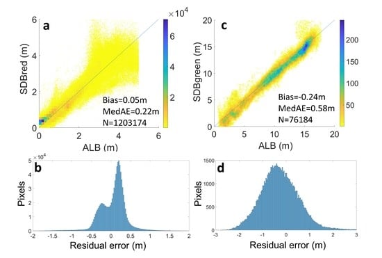
SDBgreen	0–18	−0.24	0.58	0.64	76,184
	0–5	−0.32	0.78	0.86	14,035
	5–10	−0.21	0.54	0.63	23,615
	10–18	−0.18	0.44	0.56	38,534
SDBred	0–5	0.05	0.22	0.26	1,203,174
	0–2.5	0.04	0.2	0.21	1,062,814
	2.5–5	0.07	0.45	0.55	140,360

). In shallower bins (<2.5 m), more pixels were near the 1:1 line than in deeper water, where the sensors had more difficulty detecting the bottom. The second region corresponded to West Palm. Comparison of the SDB acquired on 6 January 2017 to the ALB (Figure 2c) showed SDBgreen could consistently retrieve depths up to 18 m with a median error of 0.58 m and bias of −0.24 m; this small bias was evident in the error distribution (Figure 2d). The error was linear over most of the range until the maximum depth for validation at 18 m, and in this case, residuals showed a normal distribution (Figure 2d). In contrast, SDBgreen had slightly poorer MedAE in the shallowest water; the other depths to 18 m had essentially the same errors (Figure 2c, Table 4).

3.2. Comparison of Sentinel-3 and Sentinel-2 Products

Sentinel-3 OLCI was used in this study to examine the consistency of Sentinel-2 because its more frequent coverage allowed more comprehensive and repetitive assessments of model performance. In order to evaluate Sentinel-2 products after ACOLITE atmospheric correction, we made an intercomparison and cross-calibration of MSI against products derived from OLCI. This cross-sensor methodology is a standard procedure established in the remote sensing optical community when in situ reflectance data are not available [28,29,51]. Comparison depended on close similarity in products. OLCI- and MSI-derived outputs acquired on 8 February 2017 in Key West region are shown in Figure 3. The image pairs were taken near-simultaneously (within 45 min: OLCI at 15:22 GMT and MSI at 16:04 GMT), thus similar atmospheric and turbidity conditions could be assumed. To allow for comparable OLCI–MSI product estimations, the MSI products were aggregated to 300 m. Same day matches with low cloud cover and sunglint were rare. OLCI products (300 m, red-green-blue (RGB_ in Figure 3e), which were intended for ocean color applications, may be regarded as a radiometric-based reference for the MSI product (10 m, RGB in Figure 3f). The resulting maps of pSDB (prior to vertical referencing) allowed us to examine consistency between the sensors. The pSDB image maps were similar, although the coarse spatial resolution of OLCI (Figure 3a,c) was noticeable compared to MSI (Figure 3b,d), especially around land. In the offshore, OLCI pSDBred showed larger values (~3, Figure 3a) compared to MSI (~2.5, Figure 3b), but these data were not significant because the region corresponded to optically deep water with actual depths >30 m. The pSDBred from the two sensors (Figure 3h) compared well between low and medium values (0.7–2.5), with small bias and error (

Table 5. Statistical analyses of OLCI- and MSI-derived products acquired on 8 February 2017 in Key West. pSDB corresponds to the data prior to the vertical referencing (dimensionless) using bands 445 or 490. Remote sensing reflectance (Rrs, 1/sr) corresponds to the three red-edge bands.

Product	Bias	MedAE	n
pSDBred445 (0.7–3.2)	−0.15	0.109	21,719
pSDBed490 (0.7–3.2)	−0.33	0.26	22,091
pSDBred445 (0.7–2.5)	−0.069	0.078	18,262
pSDBred490 (0.7–2.5)	−0.17	0.14	17,157
pSDBgreen445	0.054	0.058	28,148
pSDBgreen490	−0.0023	0.016	31,858
Rrs709 & Rrs704	0.0013 1/sr	0.0014 1/sr	27,148
Rrs754 & Rrs740	0.00037 1/sr	0.00046 1/sr	15,844
Rrs779 & Rrs783	0.00062 1/sr	0.000681 1/sr	8941

) and the majority of the data laying along the 1:1 line. At pSDB depths >2.5, MSI was underestimated, consistent with a lack of detection at deeper depths because of the lower sensitivity (Table 5). Given that OLCI is an ocean color sensor, it was designed with more radiometric resolution (14-bit data) and greater sensitivity (specifically, signal-to-noise ratio, or SNR) than the MSI, a land-focused sensor; this result was expected [29]. With pSDBgreen there was no apparent difference (probably because we did not reach the maximum detectable depths for SDBgreen in this analysis), with slight overestimation by MSI (Figure 3g, Table 5). Overall, pSDBred and pSDBgreen for the two sensors agreed, the bias and MedAE were about 10% of the minimal values for pSDBred and less for pSDBgreen. Similar results were found for the comparison between pSDB using band 490 (Table 5).

The red-edge bands of Sentinel-3 and Sentinel-2, which may identify turbidity, produced equivalent results (Figure 4c–e, Table 5). MSI-derived Rrs704 (Figure 4b) and OLCI-derived Rrs709 (Figure 4a) agreed, showing a close match with no bias. The 704/709 nm bands had smaller proportional errors compared to the other bands. The bias and MAE were about 8% of the range (0.018 1/sr for 95% of the data), while the 754 and 779 nm had about twice the proportional error (against 0.037 1/sr and 0.004 1/sr, respectively). Any use of OLCI Rrs754 to approximate MSI Rrs740 (or Rrs779 to Rrs783) will require more care in dealing with the slightly greater errors. The results indicated that the ACOLITE implementation produced reasonable Rrs products over these coastal waters when the NIR–SWIR band combination was applied, consistent with previous studies on low to moderately turbid waters [29]. This knowledge is crucial for continued analysis of Sentinel-2 since Sentinel-3 will provide a control for assessing MSI consistency and will assist the temporal inspection of turbidity influence in SDB by means of the red-edge band at 709 nm (band at 704 nm for MSI).

3.3. Inspection of Turbidity Impact on Satellite-Derived Bathymetry

A temporal evaluation of the SDB products was performed in order to make a first approximation of the influence of turbidity (using the 709 nm band as a proxy) in generating false shoaling. The SDBred was examined with OLCI imagery in Key West. The model was tested using both available blue bands, 445 and 490 nm. The pSDBred was vertically referenced to the chart datum using a clear image acquired on 15 May 2017 and applied to the time series from January to August 2017 prior to Hurricane Irma. In this sense, the impact of turbidity on SDB might allow a temporal comparison of all the scenes referenced with a clear scene. Figure 5a illustrates the log–log scatter between Rrs709 and SDBred using the 445 nm band (only pixels where ALB was available were included). A clear Rrs709 maximum for each depth value is shown. This indicated the maximum depth retrievable for a given turbidity (Figure 5). The threshold equation was determined by first estimating a threshold line, then defining a linear equation for the line in log–log space. The coefficients were iteratively adjusted until 99% of the points fell below (or to the left) of the line. The linearization of the threshold resulted in Equation (2) using band 445 nm while similar results were obtained using band 490 nm (Equation (3)). The linear features in the plot were a result of quantization of the data. At extremely low values, we were reaching values where individual bits in the satellite were being distinguished, which produced a “rounding” of the data. To confirm the turbidity influence, single OLCI pixels having variable turbidity were examined over multiple scenes. An example of the relationship of turbidity limit on depth retrieval for a specific pixel at 5 m depth (Figure 5b) indicated that the threshold established (Equation (2)) from Figure 5a was consistent with a known fixed depth.

lnSDBred = −0.54 × lnRrs709 − 2.1.

(2)

lnSDBred = −0.63 × lnRrs709 − 2.56.

(3)

We applied the equation derived from OLCI (Equation (2), Figure 5a) to the MSI data (Figure 6a). The pSDBred (using band 445) was vertically referenced to the chart datum using the scene acquired on 8 February 2017. Although this exercise included few MSI images (14, see Table 2) resulting in less temporal variation in turbidity compared to OLCI time series (177 images), the number of MSI pixels was much greater with a 900-fold difference in areal resolution. A maximum of Rrs704 for each SDBred value was also encountered, where the highlighted line corresponded to the threshold defined from OLCI imagery (Figure 5a). Some pixels (3.5%) were greater than the limit. This would be expected. The MSI, with lower SNR, will have more variability. With the higher spatial variability, some residual surface reflectance (from surface waves) may also generate scatter. MSI values were higher compared to OLCI for the red-edge band (Table 5). However, the majority of MSI-derived data was located below the threshold. Note that OLCI-derived Rrs709 products ranged from ~0.000001 to 0.05 1/sr (Figure 5a), whereas MSI-derived Rrs704 had less sensitivity with a range from ~0.001 to 0.09 1/sr, approximately (Figure 6a). Figure 6b shows an example for one pixel at 10 m resolution, which corresponded to the depth of 5 m comparable to Figure 5b. The MSI data consistently followed the OLCI estimated turbidity limitation depth. The results show a potential relationship for the maximum depth retrieval for a given turbidity for this region and for the time series inspected.

The same temporal inspection of SDBgreen was accomplished in Key West with inclusion of new pixels up to ~18 m selected from charts. The pSDBgreen was vertically referenced to the chart datum using the image acquired on 15 May 2017. SDBgreen (using band 490 nm) was constrained by Rrs709 (Figure 7a), where a maximum Rrs709 followed a threshold where lnSDBgreen = −0.251 × lnRrs709 + 0.8. Using band 445 nm for SDBgreen produced an equivalent result: lnSDBgreen = −0.253 × lnRrs709 + 1.12. This threshold was not as well-defined as for SDBred; the relationship between Rrs709 and SDBgreen showed higher pixel-by-pixel scatter compared to SDBred in Key West (Figure 6b). This scatter may be due to algae absorption in addition to sediment scattering, as chlorophyll influences the blue more severely (by pigment absorption) than the green (chlorophyll was estimated with the standard OC4 blue to green band ratio algorithm). Previous work estimated the influence of the variation of chlorophyll concentration on depth estimations, suggesting that SDB methodology remained valid under a low (<1 mg/m³) and constant chlorophyll concentration (10% of variation in the image) to limit the variation of bathymetric error (15.5%) [58]. That study concluded that when the choice is possible, the scene containing the “clearest (lowest chlorophyll)” water on the training area must be retained. Following their study, we selected the boundary between low and high chlorophyll as 1 mg/m³ in three different pixels at chart depths of 8, 11, and 14 m (Figure 7b). Higher chlorophyll concentration produced shallow depths (shoaling) in the SDB independently of Rrs709.

Temporal inspection of OLCI-derived SDBgreen and chlorophyll from January to August 2017 was accomplished in West Palm Beach using the ALB depths up to 18 m. While optically shallow depth biased the OC4 chlorophyll algorithm, as they were blue:green band ratios, chlorophyll constrained the retrieved depth (Figure 8). For a known fixed depth, the chlorophyll to SDBgreen relationship shows that increasing chlorophyll does reduce the retrieved depth, just as indicated in Figure 8a. There was a clear chlorophyll limit for each depth. This relationship (determined the same way as from Figure 5a) resulted in a threshold equation: lnSDBgreen = −0.74 × lnchl + 2.48 using the blue band at 490 nm (Figure 8a). A similar equation was defined with the 445 nm (coastal blue) band: lnSDBgreen = −0.69 × lnchl + 2.73. Evaluation of individual pixel variability indicated intense shoaling patterns as chlorophyll concentration increased for each of the depths selected at 8, 10, and 15 m (Figure 8b), confirming that chlorophyll was impacting SDBgreen. No relationship was observed between SDBred and chlorophyll in Key West and West Palm Beach (results not shown).

4. Discussion

The results of this study confirmed that accurate MSI-derived bathymetric products at 10 m could be effectively retrieved using both ratio models: SDBred (ratio of the blue to red bands) for shallow water up to 5 m in Key West, and SDBgreen (ratio of the blue to green bands) for deeper areas up to 18 m (limit of lidar) in West Palm Beach (Figure 2). OLCI, with 300 m pixels, produced equivalent results (Figure 3, Table 5). Even if the Sentinel-2A/B mission might be regarded as the future of bathymetric mapping within the Sentinel constellation, the advantage of using Sentinel-3A/B is that it can provide a quick reconnaissance tool for global mapping, similar to that demonstrated with SeaWIFS (1 Km) but with a better spatial resolution [21,59]. A recent study using the SeaWIFS-derived SDB over coral reefs has confirmed that accurate bathymetric information is one of the most crucial parameters for precise flooding predictions [60]. In this sense, OLCI will allow a new perspective for global bathymetric monitoring with nine-fold better areal resolution of these strategic coral environments. In addition, a 300 m pixel can provide reliable bathymetry information and be consistent with IHO S-44 standards depending on how it is utilized [1,2]. According to NOAA, SDB has a category of zone of confidence of C or lower (CATZOC 4). NOAA’s main applications of SDB are focused on characterizing the coastal areas and monitoring seafloor changes that may have occurred since the last hydrographic survey was conducted. In this sense, SDB may be used to revise nautical charts that cannot practically be surveyed by either acoustic means or ALB. SDB information is especially helpful where vessel traffic or the deployment of navigation aids indicates that charted sounding is misleading. It should be noted that IHO S-44 standards are currently under revision, and the standards will be updated to include the ability to exploit new technologies to assist in updating nautical charts when possible.

Sentinel-2A data in these regions were extremely affected by clouds during winter and sunglint during the months around the summer solstice (Table 2), so Sentinel-3 may produce an evaluation until a usable Sentinel-2 is available. The high temporal resolution of OLCI allowed us to conduct a rapid assessment of MSI stability and atmospheric correction precision after ACOLITE processing. The frequency of revisits also provided sufficient data for temporal evaluation of SDB model performance over variable water clarity conditions (Figure 5, Figure 7 and Figure 8). Bathymetric information of shallow coastal zones is essential to the world’s management of coastal environments, economies, and cultures; yet at present, we still have incomplete and spatially limited coverage, especially over environments with transient water clarity conditions. Turbidity is one of the major constraints for good bathymetric accuracy, so identification and definition of its impact on SDB retrievals is a key step in removing biases caused by water clarity issues [2,4]. To our knowledge, documentation on how to determine and quantify the influence of turbidity on false shoaling in SDB has not been previously presented. Water quality not only varies temporally, but it also varies spatially within a scene in highly dynamic coastal regions, such as the ones analyzed here. In this study, we determined an approximation to quantify how turbidity influences the sensible depth in subtropical regions with carbonate and quartz sandy bottoms [43,44,45]. The real impact of turbidity in both OLCI and MSI was examined, establishing the maximum depth retrieved depending on the turbidity conditions by means of the red-edge bands at 709 and 704 nm for OLCI and MSI, respectively (Equations (2) and (3)). Furthermore, OLCI and MSI are not only comparable in terms of SDB but also in terms of turbidity mapping (Figure 3 and Figure 4, Table 5), highlighting the potential of the two optical missions to be interchangeable sensors for bathymetric and water monitoring. The high frequency of OLCI data permitted an understanding of the direct impact of turbidity on the limit of SDB (Figure 5); this limit can be directly transferred to MSI data (Figure 6).

The methodological framework proposed could be employed to define good practices for end users and hydrographic offices on turbidity impact. The satellite turbidity metrics could be used to determine when or where SDB may work or fail. Researchers could classify water bodies with similar water clarity characteristics relevant to SDB. Regions with constant high turbidity may be quickly clustered to provide guidance on where SDB is nonviable. Our results indicate that a suitable, operational OLCI-based turbidity index might help in selecting the likely optimal MSI images for different areas. Examination of the relationships in other environments can assess if a consistent turbidity threshold exists across multiple regions. Therefore, determining the maximum sensible depth by means of this temporal approach will provide key information for the definition of optically deep waters. The results should apply to other sensors that have red-edge bands close to 704–709 nm (e.g., WorldView-2) [36].

Another benefit of Sentinel-3 data is that water clarity and SDB from OLCI may be crucial in strategic planning for ALB missions [61]. If there is no likelihood of retrievals with Sentinel-2, efforts can move to other approaches. Turbidity information is important for ALB survey planning, and OLCI could provide climatological information that may be useful for this purpose. NOAA has applied a coastal diffuse attenuation coefficient (Kd) at 300 m that is being used in the climatology of water turbidity for lidar mission planning (www.ngs.noaa.gov/RSD/topobathy/kd2/slider.html) [62]. This climatologic product could be enhanced in the future by OLCI-derived turbidity products (Rrs709) for assessing the combined missions of ALB, SDB, and sonar.

The threshold quantified with the SDBred model showed a clear relationship between the proxy for turbidity and shoaling (Figure 5), while the limit for SDBgreen gave higher uncertainty (Figure 7). The SDBgreen scatter probably resulted from the influence of pigments (algae and other) (Figure 7 and Figure 8). One solution in the literature suggested the use of the scene containing the clearest (lowest chlorophyll) water on the training area being retained [58]. The current OLCI implementation for the default chlorophyll approach employs the standard OC4 blue to green band ratio algorithm [47]. The OC4 models use maximum band ratios of blue wavelengths, where phytoplankton absorption is strong, to green wavelengths, where phytoplankton absorption is relatively weak. It is possible that dense concentrations of algae, which absorb blue, could influence the SDBgreen. On the contrary, SDBred is less affected by algae because the absorption of both blue and red bands by algal pigments may be cancelled to some extent in the SDB. In the case of the SDBgreen model, further investigation is required in order to define the trade-off needs according to constraints in complex waters where pigment and sediment constituents vary independently. The models here considered both the 445 nm band and the 490 nm band. For SDB mapping, the 490 nm band from Sentinel-2 should be used, given that its spatial resolution is 10 m compared to the 60 m of 445 nm band.

The ratio transform required tuning of only two parameters, so few control points (less than ten) are needed. For practical application, this is a key benefit, particularly in remote areas that lack recent data. Stumpf et al. [8] used information from charts with many pre-1940 soundings that had to be re-navigated by hundreds of meters, and they still achieved mean errors of 0.2 m. A recent study demonstrated that the photon-counting lidar system, Advanced Topographic Laser Altimeter System (ATLAS) onboard the Ice, Cloud, and land Elevation Satellite-2 (ICESat-2), launched in 15 September 2018 by NASA, can retrieve valuable bathymetry in coastal and inland water body areas up to 8 m [63]. That study also suggested that bottom depth fusion from ICESat-2 and multispectral satellite imagery will be highly complementary, since ATLAS could potentially provide useful reference data for calibration (replacing soundings from nautical charts) for Sentinel-derived bathymetry in remote or poorly mapped areas. Consequently, this emerging information will generate reciprocal benefits for improved competiveness of coastal bathymetric products and their future evolution, contributing to the advancements for environmental management, monitoring, industry, navigation, modelling, and for scientific purposes, especially in developing countries.

5. Conclusions

This study used OLCI and MSI sensors to obtain bathymetric information in regions with low to moderate turbidity in South Florida. Employing widely available and free Sentinel-2 and Sentinel-3 imagery, accurate and consistent bathymetry could be retrieved when calibrated with limited available chart data. The two satellites produced equivalent results; this means that the high frequency Sentinel-3 may provide climatological information for detailed mapping with Sentinel-2. The results allowed us to identify and quantify limits on depth retrieval caused by turbidity. The 704 nm band and the OC4 chlorophyll algorithm can be proxies for turbidity and pigment impacts on SDB estimations. This is an important step toward addressing the influence of turbidity on SDB. The findings can influence several purposes such as assessing the selection of the optimal scenes, establishing the cut-off depth and the sensible depth caused by turbidity, identifying areas better suited for SDB, and developing further turbidity corrections over spatially heterogeneous waters. The twin missions and the methodology developed may benefit temporal studies requiring yearly or frequent updates of bathymetric data in rapidly varying aquatic systems such as rivers, tidal channels, underwater sand dunes, dredged ports, or after the passage of hurricanes/tropical storms. The IHO has identified the need to improve the collection, quality, and availability of hydrographic data worldwide, suggesting that shallow water bathymetry derived from multi-spectral imagery should be considered as a potential technology in areas where existing surveys are poor or non-existent. This study confirms that incorporating satellite data into forthcoming strategies will enhance our ability to retrieve bathymetry for rapid response, monitoring, and mapping of remote, dynamic, and poorly served areas of the world.

References

- International Hydrographic Review, November 2017. Report by Ian HALLS, Editor. Available online: https://www.iho.int/mtg_docs/IHReview/2017/IHR_November2017.pdf (accessed on 16 March 2019).
- International Hydrographic Publication C-55 Status of Hydrographic Surveying and Charting Worldwide. 19 October 2018. Available online: https://www.iho.int/mtg_docs/misc_docs/basic_docs/IHO_Work_Programme_for_2019_final.pdf (accessed on 16 March 2019).
- Dierssen, H.M.; Thenberge, A.E., Jr. Bathymetry: Assessing Methods. Available online: https://www.researchgate.net/profile/Heidi_Dierssen/publication/281410376_Bathymetry_Assessing_Methods/links/55e5fd7b08aecb1a7ccd625e.pdf (accessed on 16 March 2019).
- Gao, J. Bathymetric mapping by means of remote sensing: Methods, accuracy and limitations. Prog. Phys. Geogr. 2009, 33, 103–116. [Google Scholar] [CrossRef]
- Dekker, A.G.; Phinn, S.R.; Anstee, J.; Bissett, P.; Brando, V.E.; Casey, B.; Fearns, P.R.; Hedley, J.; Klonowski, W.M.; Lynch, M.; et al. Intercomparison of shallow water bathymetry, hydro-optics, and benthos mapping techniques in Australian and Caribbean coastal environments. Limnol. Oceanogr. Methods 2011, 9, 396–425. [Google Scholar] [CrossRef] [Green Version]
- Lyzenga, D.R. Shallow-water bathymetry using combined lidar and passive multispectral scanner data. Int. J. Remote Sens. 1985, 6, 115–125. [Google Scholar] [CrossRef]
- Philpot, W.D. Bathymetric mapping with passive multispectral imagery. Appl. Opt. 1989, 28, 1569–1578. [Google Scholar] [CrossRef] [PubMed]
- Stumpf, R.P.; Holderied, K.; Sinclair, M. Determination of water depth with high-resolution satellite imagery over variable bottom types. Limnol. Oceanogr. 2003, 48, 547–556. [Google Scholar] [CrossRef] [Green Version]
- Lee, Z.; Carder, K.L.; Mobley, C.D.; Steward, R.G.; Patch, J.S. Hyperspectral remote sensing for shallow waters: 2. Deriving bottom depths and water properties by optimization. Appl. Opt. 1999, 38, 3831–3843. [Google Scholar] [CrossRef] [PubMed]
- Lee, Z.; Casey, B.; Arnone, R.A.; Weidemann, A.D.; Parsons, R.; Montes, M.J.; Gao, B.-C.; Goode, W.; Davis, C.; Dye, J. Water and bottom properties of a coastal environment derived from Hyperion data measured from the EO-1 spacecraft platform. J. Appl. Remote Sens. 2007, 1, 011502. [Google Scholar] [CrossRef] [Green Version]
- Hedley, J.D.; Roelfsema, C.; Brando, V.; Giardino, C.; Kutser, T.; Phinn, S.; Mumby, P.J.; Koetz, B. Coral reef applications of Sentinel-2: Coverage, characteristics, bathymetry and benthic mapping with comparison to Landsat 8. Remote Sens. Environ. 2018, 216, 598–614. [Google Scholar] [CrossRef]
- IOCCG. Remote Sensing of Ocean Colour in Coastal, and Other Optically-Complex, Waters; IOCCG: Dartmouth, NS, Canada, 2000. [Google Scholar]
- IOCCG. Atmospheric Correction for Remotely-Sensed Ocean-Colour Products; Reports of the International Ocean-Colour Coordinating Group, No. 10, IOCCG, edited by M. Wang, 78; IOCCG: Dartmouth, NS, Canada, 2010. [Google Scholar] [CrossRef]
- Linklater, M.; Hamylton, S.M.; Brooke, B.P.; Nichol, S.L.; Jordan, A.R.; Woodroffe, C.D. Development of a seamless, high-resolution bathymetric model to compare reef morphology around the subtropical island shelves of Lord Howe Island and Balls Pyramid, southwest Pacific Ocean. Geosciences 2018, 8, 11. [Google Scholar] [CrossRef]
- Lafon, V.; Froidefond, J.M.; Lahet, F.; Castaing, P. SPOT shallow water bathymetry of a moderately turbid tidal inlet based on field measurements. Remote Sens. Environ. 2002, 81, 136–148. [Google Scholar] [CrossRef]
- Tripathi, N.K.; Rao, A.M. Bathymetric mapping in Kakinada Bay, India, using IRS-1D LISS-III data. Int. J. Remote Sens. 2002, 23, 1013–1025. [Google Scholar] [CrossRef]
- Legleiter, C.J.; Kinzel, P.J.; Overstreet, B.T. Evaluating the potential for remote bathymetric mapping of a turbid, sand-bed river: 1. Field spectroscopy and radiative transfer modeling. Water Resour. Res. 2011, 47. [Google Scholar] [CrossRef] [Green Version]
- Bramante, J.F.; Raju, D.K.; Sin, T.M. Multispectral derivation of bathymetry in Singapore’s shallow, turbid waters. Int. J. Remote Sens. 2013, 34, 2070–2088. [Google Scholar] [CrossRef]
- Pe’eri, S.; Parrish, C.; Azuike, C.; Alexander, L.; Armstrong, A. Satellite remote sensing as a reconnaissance tool for assessing nautical chart adequacy and completeness. Mar. Geod. 2014, 37, 293–314. [Google Scholar] [CrossRef]
- Favoretto, F.; Morel, Y.; Waddington, A.; Lopez-Calderon, J.; Cadena-Roa, M.; Blanco-Jarvio, A. 4SM Method Tested in the Gulf of California Suggests Field Data are Not Needed to Derive Satellite Bathymetry. Sensors 2017, 17, 2248. [Google Scholar] [CrossRef]
- Robinson, J.A.; Feldman, G.C.; Kuring, N.; Franz, B.; Green, E.; Noordeloos, M.; Stumpf, R.P. Data fusion in coral reef mapping: Working at multiple scales with SeaWiFS and astronaut photography. In Proceedings of the 6th International Conference on Remote Sensing for Marine and Coastal Environments, Charleston, SC, USA, 1–3 May 2000; Volume 2, pp. 473–483. [Google Scholar]
- Brando, V.E.; Anstee, J.M.; Wettle, M.; Dekker, A.G.; Phinn, S.R.; Roelfsema, C. A physics based retrieval and quality assessment of bathymetry from suboptimal hyperspectral data. Remote Sens. Environ. 2009, 113, 755–770. [Google Scholar] [CrossRef]
- Kutser, T.; Paavel, B.; Verpoorter, C.; Ligi, M.; Soomets, T.; Toming, K.; Casal, G. Remote sensing of black lakes and using 810 nm reflectance peak for retrieving water quality parameters of optically complex waters. Remote Sens. 2016, 8, 497. [Google Scholar] [CrossRef]
- Toming, K.; Kutser, T.; Laas, A.; Sepp, M.; Paavel, B.; Nõges, T. First experiences in mapping lake water quality parameters with Sentinel-2 MSI imagery. Remote Sens. 2016, 8, 640. [Google Scholar] [CrossRef]
- Vanhellemont, Q.; Ruddick, K. Acolite for Sentinel-2: Aquatic applications of MSI imagery. In Proceedings of the ESA Living Planet Symposium, Prague, Czech Republic, 9–13 May 2016. [Google Scholar]
- Martins, V.S.; Barbosa, C.C.F.; de Carvalho, L.A.S.; Jorge, D.S.F.; Lobo, F.D.L.; Novo, E.M.L.D.M. Assessment of Atmospheric Correction Methods for Sentinel-2 MSI Images Applied to Amazon Floodplain Lakes. Remote Sens. 2017, 9, 322. [Google Scholar] [CrossRef]
- Ruddick, K.; Vanhellemont, Q.; Dogliotti, A.; Nechad, B.; Pringle, N.; Van der Zande, D. New opportunities and challenges for high resolution remote sensing of water colour. In Proceedings of the Ocean Optics 2016, Victoria, CB, Canada, 2 October 2016. [Google Scholar]
- Pahlevan, N.; Schott, J.R.; Franz, B.A.; Zibordi, G.; Markham, B.; Bailey, S.; Schaafe, C.B.; Ondrusek, M.; Greb, S.; Strait, C.M. Landsat 8 remote sensing reflectance (Rrs) products: Evaluations, intercomparisons, and enhancements. Remote Sens. Environ. 2017, 190, 289–301. [Google Scholar] [CrossRef]
- Pahlevan, N.; Sarkar, S.; Franz, B.A.; Balasubramanian, S.V.; He, J. Sentinel-2 MultiSpectral Instrument (MSI) data processing for aquatic science applications: Demonstrations and validations. Remote Sens. Environ. 2017, 201, 47–56. [Google Scholar] [CrossRef]
- Chybicki, A. Mapping South Baltic Near-Shore Bathymetry Using Sentinel-2 Observations. Pol. Marit. Res. 2017, 24, 15–25. [Google Scholar] [CrossRef] [Green Version]
- Kabiri, K. Discovering optimum method to extract depth information for nearshore coastal waters from Sentinel-2A imagery-case study: Nayband Bay, Ian. In Proceedings of the International Archives of the Photogrammetry, Remote Sensing & Spatial Information Sciences XLII-4/W4, 42, Tehran’s Joint ISPRS Conferences of GI Research, SMPR and EOEC 2017, Tehran, Iran, 7–10 October 2017. [Google Scholar]
- Traganos, D.; Reinartz, P. Mapping Mediterranean seagrasses with Sentinel-2 imagery. Mar. Pollut. Bull. 2017, 134, 197–209. [Google Scholar] [CrossRef]
- Casal, G.; Monteys, X.; Hedley, J.; Harris, P.; Cahalane, C.; McCarthy, T. Assessment of empirical algorithms for bathymetry extraction using Sentinel-2 data. Int. J. Remote Sens. 2018, 1–25. [Google Scholar] [CrossRef]
- European Commission. Copernicus for Coastal Zone Monitoring and Management Workshop; Technical Report; Copernicus Support Office: Brussels, Belgium, 2017.
- Traganos, D.; Poursanidis, D.; Aggarwal, B.; Chrysoulakis, N.; Reinartz, P. Estimating satellite-derived bathymetry (SDB) with the google earth engine and sentinel-2. Remote Sens. 2018, 10, 859. [Google Scholar] [CrossRef]
- Halls, J.; Costin, K. Submerged and Emergent Land Cover and Bathymetric Mapping of Estuarine Habitats Using WorldView-2 and LiDAR Imagery. Remote Sens. 2016, 8, 718. [Google Scholar] [CrossRef]
- Islam, S.; Hasan, Z.; Islam, A. The Challenges of River Bathymetry Survey Using Space Borne Remote Sensing in Bangladesh. Atmos. Ocean. Sci. 2016, 1, 7–13. [Google Scholar] [CrossRef]
- Kabiri, K. Accuracy assessment of near-shore bathymetry information retrieved from Landsat-8 imagery. Earth Sci. Inform. 2017, 10, 235–245. [Google Scholar] [CrossRef]
- Hamylton, S.M.; Hedley, J.D.; Beaman, R.J. Derivation of high-resolution bathymetry from multispectral satellite imagery: A comparison of empirical and optimisation methods through geographical error analysis. Remote Sens. 2015, 7, 16257–16273. [Google Scholar] [CrossRef]
- Jones, R.; Boyer, J.N. Florida Keys National Marine Sanctuary Water Quality Monitoring Project: 1998 Annual Report; Florida International University: Miami, FL, USA, 1988. [Google Scholar]
- Lapointe, B.E.; Clark, M. Nutrient inputs from the watershed and coastal eutrophication in the Florida Keys. Estuar. Coasts 1992, 15, 465–476. [Google Scholar] [CrossRef]
- Barnes, B.B.; Hu, C. A hybrid cloud detection algorithm to improve MODIS sea surface temperature data quality and coverage over the Eastern Gulf of Mexico. IEEE Trans. Geosci. Remote Sens. 2013, 51, 3273–3285. [Google Scholar] [CrossRef]
- Fourqurean, J.W.; Zieman, J.C.; Powell, G.V. Phosphorus limitation of primary production in Florida Bay: Evidence from C: N: P ratios of the dominant seagrass Thalassia testudinum. Limnol. Oceanogr. 1992, 37, 162–171. [Google Scholar] [CrossRef]
- Finkl, C.W.; Benson, R.; Yuhr, L. Demonstration of Feasibility of Using the “Geomorphic Site Selection Software Tool” by Comparison to Known Conditions along the Southeast Florida Coast; Technos, Inc.: Holland, MI, USA, 1997; Task 4 Report for Naval Facilities Engineering Command, Port Hueneme, California (Contract No. N47408-96-C-7226, Line No. 001AD). [Google Scholar]
- Finkl, C.W.; Warner, M.T. Morphologic features and morphodynamic zones along the inner continental shelf of southeastern Florida: An example of form and process controlled by lithology. J. Coast. Res. 2005, 42, 79–96. [Google Scholar]
- European Space Agency. Sentinel-3 OLCI Technical Guide. Available online: https://sentinel.esa.int/web/sentinel/user-guides/sentinel-3-olci (accessed on 30 May 2018).
- O’Reilly, J.E.; Maritorena, S.; Siegel, D.A.; O’Brien, M.C.; Toole, D.; Mitchell, B.G.; Kahru, M.; Chavez, F.; Strutton, P.G.; Cota, G.F.; et al. Ocean color chlorophyll a algorithms for SeaWiFS, OC2, and OC4: Version 4. SeaWiFS post launch calibration and validation analyses; Goddard Space Flight Center: Greenbelt, MD, USA, 2000; Part 3; pp. 9–23.
- Werdell, P.J.; Bailey, S.W. An improved bio-optical data set for ocean color algorithm development and satellite data product validation. Remote Sens. Environ. 2005, 98, 122–140. [Google Scholar] [CrossRef]
- European Space Agency. Sentinel-2 User Handbook; ESA Standard Document 2015; European Space Agency: Paris, France, 2015. [Google Scholar]
- Vanhellemont, Q.; Ruddick, K. Turbid wakes associated with offshore wind turbines observed with Landsat 8. Remote Sens. Environ. 2014, 145, 105–115. [Google Scholar] [CrossRef] [Green Version]
- Vanhellemont, Q.; Ruddick, K. Advantages of high quality SWIR bands for ocean colour processing: Examples from Landsat-8. Remote Sens. Environ. 2015, 161, 89–106. [Google Scholar] [CrossRef] [Green Version]
- Belkin, I.M.; O’Reilly, J.E. An algorithm for oceanic front detection in chlorophyll and SST satellite imagery. J. Mar. Syst. 2009, 78, 319–326. [Google Scholar] [CrossRef]
- Hu, C.; Chen, Z.; Clayton, T.D.; Swarzenski, P.; Brock, J.C.; Muller-Karger, F.E. Assessment of estuarine water-quality indicators using MODIS medium-resolution bands: Initial results from Tampa Bay, FL. Remote Sens. Environ. 2004, 93, 423–441. [Google Scholar] [CrossRef]
- Chen, Z.; Hu, C.; Muller-Karger, F. Monitoring turbidity in Tampa Bay using MODIS/Aqua 250-m imagery. Remote Sens. Environ. 2007, 109, 207–220. [Google Scholar] [CrossRef]
- Liu, H.; Li, Q.; Shi, T.; Hu, S.; Wu, G.; Zhou, Q. Application of sentinel 2 MSI images to retrieve suspended particulate matter concentrations in Poyang Lake. Remote Sens. 2017, 9, 761. [Google Scholar] [CrossRef]
- Drusch, M.; Gascon, F.; Berger, M. GMES Sentinel-2 Mission Requirements Document; ESA: Frascati, Italy, 2010; EOP-SM1163MR-Dr242. [Google Scholar]
- Seegers, B.N.; Stumpf, R.P.; Schaeffer, B.A.; Loftin, K.A.; Werdell, P.J. Performance metrics for the assessment of satellite data products: An ocean color case study. Opt. Express 2018, 26, 7404–7422. [Google Scholar] [CrossRef] [PubMed]
- Minghelli-Roman, A.; Dupouy, C. Influence of water column chlorophyll concentration on bathymetric estimations in the lagoon of New Caledonia, using several MERIS images. IEEE J. Sel. Top. Appl. Earth Obs. Remote Sens. 2013, 6, 739–745. [Google Scholar] [CrossRef]
- Stumpf, R.P.; Feldman, G.; Kuring, N.; Franz, B.; Green, E.; Robinson, J. SeaWiFS spies reefs. Reef Encount. 1999, 26, 29–30. [Google Scholar]
- Beck, M.W.; Losada, I.J.; Menéndez, P.; Reguero, B.G.; Díaz-Simal, P.; Fernández, F. The global flood protection savings provided by coral reefs. Nat. Commun. 2018, 9, 2186. [Google Scholar] [CrossRef] [PubMed]
- Saylam, K.; Brown, R.A.; Hupp, J.R. Assessment of depth and turbidity with airborne Lidar bathymetry and multiband satellite imagery in shallow water bodies of the Alaskan North Slope. Int. J. Appl. Earth Obs. Geoinf. 2017, 58, 191–200. [Google Scholar] [CrossRef]
- Tomlinson, M.C.; Stumpf, R.P.; Vogel, R.L. Approximation of diffuse attenuation, Kd, for MODIS high-resolution bands. Remote Sens. Lett. 2019, 10, 178–185. [Google Scholar] [CrossRef]
- Forfinski-Sarkozi, N.A.; Parrish, C.E. Analysis of MABEL Bathymetry in Keweenaw Bay and Implications for ICESat-2 ATLAS. Remote Sens. 2016, 8, 772. [Google Scholar] [CrossRef]