Article

Using Hidden Markov Models for Land Surface Phenology: An Evaluation Across a Range of Land Cover Types in Southeast Spain

by
Miguel A. García
1,
Hassane Moutahir
2,
Grant M. Casady
3,
Susana Bautista
2 and
Francisco Rodríguez
4,*
1
Department of Applied Mathematics, University of Alicante, Apdo. 99, 03080 Alicante, Spain
2
Department of Ecology and Multidisciplinary Institute for Environmental Studies (IMEM), University of Alicante, Apdo. 99, 03080 Alicante, Spain
3
Department of Biology, Whitworth University, 300 W. Hawthorne Road, Spokane, WA 99251, USA
4
Department of Applied Mathematics and Multidisciplinary Institute for Environmental Studies (IMEM), University of Alicante, Apdo. 99, 03080 Alicante, Spain
*
Author to whom correspondence should be addressed.
Remote Sens. 2019, 11(5), 507; https://doi.org/10.3390/rs11050507
Submission received: 23 December 2018 / Revised: 18 February 2019 / Accepted: 1 March 2019 / Published: 2 March 2019
(This article belongs to the Special Issue Land Surface Phenology )

Abstract

:
Land Surface Phenology (LSP) metrics are increasingly being used as indicators of climate change impacts in ecosystems. For this purpose, it is necessary to use methods that can be applied to large areas with different types of vegetation, including vulnerable semiarid ecosystems that exhibit high spatial variability and low signal-to-noise ratio in seasonality. In this work, we evaluated the use of hidden Markov models (HMM) to extract phenological parameters from Moderate Resolution Imaging Spectroradiometer (MODIS) derived Normalized Difference Vegetation Index (NDVI). We analyzed NDVI time-series data for the period 2000–2018 across a range of land cover types in Southeast Spain, including rice croplands, shrublands, mixed pine forests, and semiarid steppes. Start of Season (SOS) and End of Season (EOS) metrics derived from HMM were compared with those obtained using well-established smoothing methods. When a clear and consistent seasonal variation was present, as was the case in the rice croplands, and when adjusting average curves, the smoothing methods performed as well as expected, with HMM providing consistent results. When spatial variability was high and seasonality was less clearly defined, as in the semiarid shrublands and steppe, the performance of the smoothing methods degraded. In these cases, the results from HMM were also less consistent, yet they were able to provide pixel-wise estimations of the metrics even when comparison methods did not.

Graphical Abstract

1. Introduction

Land Surface Phenology (LSP), the seasonal pattern of variation in vegetated land surfaces observed from remote sensing [1,2], has been proven in the last decades to be a basic tool to investigate climate change impacts in ecosystems (e.g., References [3,4,5]). The availability of long time series of vegetation indices derived from different space-borne sensors has allowed for the description of phenology metrics at global, regional, or local scales, and to analyze their spatio-temporal changes in relation to climate trends and human or natural disturbances (e.g., References [4,5,6,7,8,9,10,11,12,13,14]).
Moderate Resolution Imaging Spectroradiometer (MODIS) derived vegetation index (VI) time series have provided a convenient balance between the length of the available time series and temporal and spatial resolution, being available at 250 m pixel size, every 16 days since the year 2000 [7,15,16], which is suitable for describing and analyzing seasonal patterns and trends in regional-to-global LSP metrics.
Normalized Difference Vegetation Index (NDVI) is the most commonly used vegetation index to extract phenology metrics, although alternative vegetation indices can also be used and their possible advantages and drawbacks to derive phenology metrics in specific land cover types have been discussed (e.g., References [17,18,19]). Different methods have been proposed to extract phenological parameters from NDVI or other VI time series (e.g., References [6,7,20,21,22,23,24]; see a review in Reference [25]), with some form of smoothing method, polynomial or model function fitting, and threshold or inflexion point estimation being the most commonly employed strategy, with active discussion on the performance of the different methodologies [26,27].
Hidden Markov models (HMM) constitute a modeling technique for sequential data. A clear exposition of basic concepts about HMM can be found in Reference [28]; to facilitate reading, the basis of HMM is recalled in Section 2.1. HMM were originally developed in the field of automatic speech recognition [28], where they constitute the basis of large vocabulary continuous speech recognition systems [29]. HMM have found wider applications in a variety of fields, such as climatology [30,31], image analysis [32], psychology [33,34], ecology [35,36,37,38,39,40], and especially in bioinformatics, where HMM have provided the basis for many applications and software tools [41,42,43,44]. In the field of remote sensing, the use of HMM has been mainly restricted to image analysis and landscape classification [45,46,47,48,49,50,51,52,53].
HMM were proposed more than two decades ago by Viovy and Saint [54] as a useful method to obtain LSP metrics. However, alternative methods of analysis were preferred at the time, and only recently, a very limited use of HMM for applications in LSP can be found. Cerqueira Leite et al. [47] and Siachalou et al. [49] used HMM modeling of crop phenology with the aim of classifying different types of crops from time series of remote sensed images. Shen et al. [55] used HMM modeling of corn phenological phases to estimate corn progress from NDVI and meteorological data. García et al. [56] discussed the application of HMM to extract LSP metrics from the time series of NDVI data. Given the successful experiences with applications of HMM based methods in different fields in the last decades, as well as the expansion in computing capabilities that allows for efficient implementation in any modern desktop computer, it is timely to reconsider the use of HMM for LSP and to test their performance in comparison with usual methodologies. There are two main expected potential advantages in the use of HMM to derive LSP metrics. Firstly, as discussed in Reference [56], HMM can model the different phenological states of the vegetation and the transitions between them, and so they could be tailored to include a priori information about the phenology of specific types of vegetation or land cover types. Secondly, should the estimation of LSP metrics using basic types of HMM provide satisfactory results, there would be wide opportunities for further improvements, as there are many variants and extensions of HMM that have already been employed in related signal analysis problems (see, e.g., References [29,42]).
The aim of this paper is to evaluate the potential of using HMM to derive LSP metrics from time series of vegetation indices. To this end, we analyzed NDVI time series data for the period 2000–2018 across a range of land cover types in Southeast Spain, including rice croplands, shrublands, mixed pine forests, and semiarid steppes, obtaining SOS and EOS metrics derived from HMM that were compared with those obtained using well-established smoothing methods. Our main objective was to check the feasibility of applying HMM to large areas with different types of vegetation, including semiarid ecosystems that exhibit high spatial variability and low signal-to-noise ratio in seasonality, where smoothing methods could possibly fall short of exhibiting the best performance.
From the results obtained in this work, we concluded that phenology metrics derived from the simple type of HMM, considered in this paper, were consistent with those obtained from commonly employed smoothing methods, that they were able to provide metrics estimations for all pixels even in some cases where smoothing methods partly failed, and that they showed correlations with climate variables in a similar way to the best smoothing methods, suggesting the validity of the HMM derived metrics.

2. Materials and Methods

2.1. Hidden Markov Models Basis
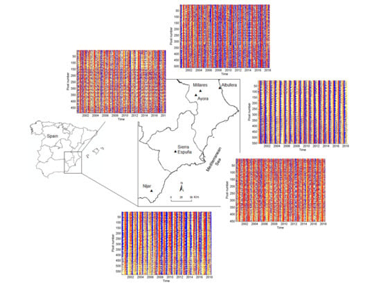
For the sake of clarity, we recall in this section the basic elements of HMM, in the context of their use in this paper. More general and detailed descriptions can be found in References [28,54]. For technical aspects of inference and algorithms, we refer the reader to the specialized literature (see, e.g., Reference [57]).
An HMM consists of a sequence of observable states, {Yt}, a sequence of unobservable or hidden states, {St}, and two probabilistic models determining how both sequences are generated (Figure 1a). The observable states, called “emissions” from the origins of HMM in the field of speech recognition, correspond in this paper to a time series of NDVI increments. The probability distributions of these observed states depend on the hidden states (Figure 1a), which could refer to the corresponding “phenological states” of the vegetation, i.e., growing, declining, or stationary. We assume that, for a given hidden state, the observed NDVI increments follow a Gaussian distribution whose mean and standard deviation depend solely on the hidden state. Thus, for instance, the expected mean values of NDVI changes would be positive or negative for the growing or declining hidden states, respectively. The probabilistic model for the sequence of hidden states is a Markov chain, defined by the transition probabilities between states. The basic type of HMM used in this paper is a first order HMM (Figure 1a), where the transition probabilities from a hidden state to any other depend only on the current state, and not on the history of the system. Thus, in Figure 1a, the absence of an arrow connecting two states, hidden or observed, implies their conditional independence, so that, given St, both St+1 and Yt are independent of previous hidden or observed states.
The so-called topology of the HMM is defined when the number of hidden states is given, as well as the possible existence of forbidden transitions between states (called blocking). Figure 1b presents the topology of the HMM used in this work, an HMM with four states, increasing (S+), stationary high (S0+), decreasing (S), and stationary low (S0−), with transitions between states only allowed for those connected with arrows. Since the sum of the transition probabilities from a given hidden state to any other is one, there are only four independent transition probabilities. In total, there are twelve independent parameters in the model, as for each of the four hidden states the Gaussian density for the emissions is defined by its mean and standard deviation.
Once the topology of the HMM is defined, as well as the type of probability distributions for the emissions, given a sequence of observed states the parameters of the model can be fitted using an expectation maximization algorithm [58,59] that provides the values of the parameters that maximize the likelihood of the observations. Then, having values for the parameters of the model, the sequence of hidden states can be inferred using a dynamic programming algorithm known as the Viterbi algorithm [60]. In this way, given a time series of NDVI changes, phenology metrics such as the Start of Season (SOS) and End of Season (EOS) can be defined from the inferred sequence of hidden states, as SOS and EOS would correspond to some moments where the hidden state of the system is S+ or S, respectively.

2.2. Study Areas

Five study areas in Southeast Spain, located in three different regions, were selected from general on-the-ground information regarding their predominant land cover types (Figure 2). In Valencia region, Albufera site comprises an area of traditional rice crops surrounding a coastal lagoon; Millares and Ayora sites are inland mountain areas, with altitudes ranging from 600 to 800 m in Millares, and 700 to 1000 m in Ayora, with vegetation cover dominated by shrublands. In Murcia region, Espuña site, located in Espuña range, with altitudes ranging from 650 to 1300 m, is a mixed pine forest derived from a reforestation project dating back to the end of the 19th century. In Andalucía region, the Níjar site is located close to the Southern Mediterranean coast, with altitudes ranging from 250 to 900 m with grass steppes as the main land cover.
In each study area, around 500 MODIS pixels were visually selected using Google EarthTM images, which provided enough resolution to try to avoid areas with heterogeneous land cover (e.g., crops in areas of natural vegetation, very steep slopes in mountain areas, and civil constructions) without the need of any special software for image analysis. Approximate central coordinates and number of selected pixels for each site are shown in Table 1; kmz files showing the grid of pixels for each area are included as supplementary material (File S1).

2.3. Data Adquisition

MODIS data were downloaded from the Land Processes Distributed Active Archive Center (LP DAAC, https://lpdaac.usgs.gov/) managed by the NASA Earth Science Data and Information System (ESDIS) project. We used a time series of NDVI data, from MODIS product MOD13Q1 Version 6 [16], corresponding to the best pixels in 16 day intervals (NDVI 16-days composite band) at 250 m resolution, from February 2000 to June 2018. This data is stored in scientific data sets (SDS) under the NASA Hierarchical Data Format Earth Observing System (HDF-EOS) format, which is the standard archive format for all EOS Data Information System (EOSDIS) products [16]. We used the NASA Application for Extracting and Exploring Analysis Ready Samples (AρρEEARS) and R software to access and download the NDVI-MODIS data. Pixel-reliability (PR) and Day-of-the-year (DOY) layers were also downloaded and used in some analyses. PR provides a rank of the overall quality of the pixel, and DOY provides the actual date of acquisition of the reflectance’s used to compute each pixel NDVI.
Climate data were obtained from the Agroclimatic Information System for Irrigation (SiAR) network, Spanish Ministry of Agriculture, Fisheries and Food (http://eportal.mapama.gob.es/websiar/).

2.4. Methods of Analysis

General statistical analyses, including descriptive statistics, and correlation and regression analyses, were carried out using the software R [61].

2.4.1. Pixel Homogeneity Check

We checked similarity in phenological behaviors of the selected pixels in each study area, by decomposing the time series of NDVI for each pixel (NDVI curve) as the sum of a trend or secular component (computed as the average in a moving window of size corresponding to one year) and an annual component, and computing correlations between the annual component for each pixel and the average for the whole area (mean annual curve).

2.4.2. Hidden Markov Models Fitting and Analysis

For each NDVI curve, data with NA values or with PR > 1 were excluded. Using DOY data, NDVI values were interpolated every four days, and a mild smoothing with kernels [0.0370, 0.1111, 0.2222, 0.2593, 0.2222, 0.1111, and 0.0370] was applied. From the resulting equally spaced NDVI time series, finite differences were computed. The set of finite differences series for all pixels in each study area was used to fit a four state HMM with blocking (Figure 1b) and Gaussian emissions, using the HMM Toolbox for MatlabTM [62]. For each study area, once the fitted parameters were obtained, Viterbi algorithm was applied to obtain the most probable sequence of hidden states for each pixel. Finally, for each pixel and season, SOS (respectively, EOS) was defined to be the day of the year corresponding to a given percentile (25 or 50) in the series of hidden S+ states (respectively, S).

2.4.3. Phenology Metrics Using Smoothing Methods

Two different tools, based on smoothing methods and commonly used to extract phenology metrics, were employed to compare HMM results: The R package greenbrown [63,64,65] and the stand-alone program TIMESAT [22,66].
Phenology analyses with the R package greenbrown were carried out, excluding NDVI values with PR > 1, in an automated way using the package function “Phenology” with default parameters. As described in Reference [64], this function performs three successive steps: 1) Filling gaps in the time series; 2) smoothing and interpolation; and 3) extraction of phenology metrics SOS and EOS. Three different methods of smoothing and interpolation were applied, using linear interpolation, splines, or double logistic functions; the resulting metrics from each method are denoted in what follows as gb_lin, gb_spl, and gb_dbl, respectively. For the SOS and EOS definitions, we used the approach “white” [67], based on 50% thresholds between minimum and maximum NDVI values.
For TIMESAT analyses, NDVI values were first weighted according to PR, such that values with a reliability of 0 (“good data”) were weighted as 1, reliability of 1 (“marginal data”) were weighted as 0.5, and all other reliability values were weighted as 0.1. Second, the data were smoothed by removing spikes from the time series. Spikes were identified as observations that deviated from the median of a moving window by more than one standard deviation. Once the time series was cleaned and smoothed, we used a double logistic fitting method to describe the seasonal curve, as described by Zhang et al. [7]. SOS and EOS were established as 20% of the annual amplitude.

3. Results

3.1. Homogeneity Analysis and Seasonality Behavior in Different Land Cover Types

Homogeneity analysis showed generally high correlation values between NDVI seasonal curves for each pixel and the mean curve in each study area, as illustrated, for example, in Figure 3 for Níjar site; similar figures for the other study areas are included as supplementary material (Figure S1). As seen in Figure 3, there is certain variability in correlation values, probably related in this site with differences in slope aspect; in other areas (Figure S1) there are also a few pixels having lower correlations with the mean seasonal curve; however, no areas exhibiting markedly different phenology behaviors were detected in any of the sites.
Mean NDVI curves, showing different seasonal behaviors in croplands and in natural vegetation are presented in Figure 4. While in rice crops (Figure 4a) a clear and consistent intra-year seasonal variation was present, in the areas with natural vegetation (Figure 4b–e) seasonality was essentially defined by the extreme dry conditions in summer, with very low precipitation and high temperatures. Thus, in natural areas, seasons extended through two consecutive years, and a high variability between different seasons was present.

3.2. Estimated Hidden Markov Models Parameters and Inferred Hidden States

Parameters for HMM estimated for each study area are presented in Table 2. As shown in Table 2, HMM parameters reflect the differences in NDVI seasonality between croplands and natural vegetation, with higher values in Albufera, the site with rice crops, for transition probabilities between identical states, implying more well-defined sequences of states, and also much higher absolute values for mean NDVI changes (emissions) in the states corresponding to NDVI increasing (S+) and decreasing (S) values.
For each study area, inferred hidden states for each pixel in the area are presented in Figure 5.
As clearly shown in Figure 5, inferred states in croplands exhibit short and well-defined compact growing seasons (Figure 5a, red), consistent across pixels and years, which also applies with a bit more variability to declining states (Figure 5a, blue). In natural land cover types (Figure 5b–e) seasons are much less defined, extend wider in time, and present a much higher variability both between pixels and between different years.

3.3. Comparison of Phenology Metrics Derived from Hidden Markov Models and Smoothing Methods

In rice crops, where growing and declining seasons are marked and short, we defined HMM-derived SOS and EOS as the median (50th percentile) of DOY with corresponding inferred hidden states (S+ and S, respectively).
Table 3 presents Pearson correlation coefficients between mean SOS and EOS values (averages of SOS or EOS for all pixels) derived from different methods in Albufera site. Correlations vary in magnitude and significance between different pair comparisons, with those corresponding to HMM derived SOS showing, in general, intermediate values, significant in most cases, and lower values for EOS, but still significant when compared to greenbrown with linear interpolation.
For the study areas with natural land cover types, with more fuzzy and extended seasons, we defined SOS and EOS from HMM as the first quartile (25th percentile) of DOY with hidden states S+ and S, respectively. Correlations between HMM derived SOS in these areas, in comparison with those derived from other methods, are presented in Table 4. Correlation coefficients for phenology metrics from HMM and TIMESAT showed high values, which were highly significant in all cases. Comparisons between either HMM or TIMESAT and the other three methods showed rather similar correlations in all four land cover types.

3.4. Performance of the Methods on Phenology Metrics Definition and Variability

We analyzed, for each method, site and year, the number of pixels where the method was not able to derive a defined metric, resulting in a NA (not available) metric. Table 5 shows the proportion of NA pixels for SOS metric, as the average over all the years. SOS metrics derived from HMM are always defined, as they only depend on the presence of inferred growing states. Except for TIMESAT in Albufera, there are always a certain proportion of pixels with NA metrics for the different smoothing methods, usually higher in natural land cover types.
Mean yearly values of coefficients of variation (COV) among pixels, for the different study areas and methods, are presented in Table 6. While a higher variability among pixels in different areas could reflect a real higher spatial variability, higher values of COV could also be the result of a lower performance in the precision of the estimation method. As shown in Table 6, HMM and TS metrics exhibited, in most cases, lower values of COV, with either of them being the lowest depending on the study area.

3.5. Relation of Phenology Metrics with Climate Variables

Lacking on-the-ground phenology measurements to compare with those from LSP, the presence of significant relations between LSP derived metrics and climate variables, as well as their magnitudes, could be considered as indicative of their validity. Figure 6 presents the relations between HMM derived SOS metrics and selected climate variables in Níjar site, showing significant linear dependencies, with previous cumulative precipitation being related to earlier SOS, while differences in temperature between September and spring were related to higher values.
Coefficients of determination (r2 values) for similar relations between SOS metrics derived from different methods and climate variables are presented in Table 7. Apart from significant relations for HMM derived SOS with both precipitation and temperature, of the different smoothing methods only TS derived SOS was significantly related with precipitation, and in all cases their relations exhibited lower r2 values than those from HMM.

4. Discussion

HMM derived phenology metrics, in different land cover types, were consistent with those derived from usual smoothing methods, providing estimations for all pixels in all of the study areas considered in this work, even when comparison methods did not.
Usual curve fitting methods can be applied either to NDVI mean curves for a whole area or to individual pixel curves. In the first case, no information on the spatial distribution of phenology metrics is obtained, while in the second, the fitting of individual curves might result in high variances and the lack of metrics for a number of pixels, especially with noisy individual NDVI curves. Conversely, there are two scales involved in the HMM fitting process. Given an area with homogeneous NDVI behavior, the whole set of pixels in the area can be used to obtain estimations of the HMM parameters, which makes the estimation process and the resulting model very robust. This model is then used to infer the sequence of hidden states for each pixel in the area, which is the base to obtain the LSP metrics at the pixel level.
The spatial distribution of the resulting HMM derived metrics is expected to be well-behaved, assuming that NDVI curves in the area are sufficiently homogeneous. In this work, we wanted to evaluate the use of HMM for LSP in different land cover types, and so we selected a priori homogeneous areas, and also checked, a posteriori, their homogeneity. In general, as suggested and carried out in References [54,56], HMM could be applied in large heterogeneous areas by using a previous automatic clustering process of the pixels based on NDVI similarities.
Despite the HMM being proposed very early as a tool to investigate vegetation dynamics from remote sensing observations [54], and although there have been a few examples of applications of HMM in phenology in recent years [47,49,55,56], to our knowledge there has been no previous published evaluation of the performance of HMM to define phenology metrics in comparison with other methods. In this work we have employed a very simple model of HMM and tested its ability to provide phenology metrics in comparison to ready applications of different smoothing methods, without trying to optimize any of the methods or adjusting them to particular study areas. Thus, our results should not be considered as an evaluation of the smoothing methods used as reference, but as indication that HMM are able to provide consistent results.
Since NDVI and vegetation phenology are expected to be related to climate variables (e.g., References [68,69]), the relations of SOS derived from HMM and other methods with climate variables presented in Figure 6 and Table 7 are indications of the validity of HMM derived metrics. Notwithstanding, further work including comparisons with ground-based data would be required to confirm these indications. The results presented in this paper strongly support the potential of HMM as an alternative or complementary method for deriving LSP metrics, thus opening new lines of research and possible improvements by using many of the variants and extensions of the basic type of HMM used in this work. For instance, we have used the same topology of the HMM in all land cover types, but they could be adapted to particular areas with different vegetation types, either in the number of states or the allowed transitions between states. Additionally, we have employed homogeneous HMM, i.e., with transition probabilities between states constant in time, but they can be allowed to be time-dependent [55]. More complex models, as higher order or semi-Markov models [70], could also be used to model the duration of the different phases of the season.

5. Conclusions

Our results show that HMM derived phenology metrics can be obtained in large areas with different land cover types, producing consistent values with those obtained from commonly employed smoothing methods. HMM were able to provide metrics estimations for all pixels, while smoothing methods partly failed in some cases. Spatial variability of HMM metrics were similar to the best behaving smoothing method, and lower than other methods in many cases. Correlations of HMM derived SOS metrics with climate variables were similar or higher than those with the best smoothing methods, suggesting the validity of the HMM derived metrics. As a general conclusion, our results indicate that HMM can be very useful for the derivation of LSP metrics, providing pixel-wise estimations in large areas, although further work is needed to assess their performance in relation with on-the-ground observations.

Supplementary Materials

The following are available online at https://www.mdpi.com/2072-4292/11/5/507/s1, Figure S1: Correlations between annual component of NDVI time series for each pixel and global mean annual curve in Albufera, Millares, Ayora, and Espuña sites, File S1: Compressed file including kmz files for the five study areas.

Author Contributions

Conceptualization, M.A.G, F.R. and S.B.; Methodology and Formal Analysis, M.A.G., H.M., G.M.C. and F.R.; Writing-Original Draft Preparation, F.R.; Writing-Review & Editing, all the authors; Visualization, M.A.G. and H.M.; Funding Acquisition, F.R. and S.B.

Funding

This research was funded by Ministerio de Economía y Competitividad grant numbers CGL2017-89804-R, CGL2014-59074-R, and CGL2015-69773-C2-1-P.

Conflicts of Interest

The authors declare no conflict of interest. The funders had no role in the design of the study; in the collection, analyses, or interpretation of data; in the writing of the manuscript, and in the decision to publish the results.

References

  1. Reed, B.C.; Brown, J.F.; Vanderzee, D.; Loveland, T.R.; Merchant, J.W.; Ohlen, D.O. Measuring phenological variability from satellite imagery. J. Veg. Sci. 1994, 5, 703–714. [Google Scholar] [CrossRef]
  2. Helman, D. Land surface phenology: What do we really ‘see’ from space? Sci. Total Environ. 2018, 618, 665–673. [Google Scholar] [CrossRef] [PubMed]
  3. Morisette, J.T.; Richardson, A.D.; Knapp, A.K.; Fisher, J.I.; Graham, E.A.; Abatzoglou, J.; Wilson, B.E.; Breshears, D.D.; Henebry, G.M.; Hanes, J.M.; et al. Tracking the rhythm of the seasons in the face of global change: Phenological research in the 21st century. Front. Ecol. Environ. 2009, 7, 253–260. [Google Scholar] [CrossRef]
  4. Ivits, E.; Cherlet, M.; Tóth, G.; Sommer, S.; Mehl, W.; Vogt, J.; Micale, F. Combining satellite derived phenology with climate data for climate change impact assessment. Glob. Planet. Chang. 2012, 88–89, 85–97. [Google Scholar] [CrossRef]
  5. Garonna, I.; Jong, R.; Schaepman, M.E. Variability and evolution of global land surface phenology over the past three decades (1982–2012). Glo. Chang. Biol. 2016, 22, 1456–1468. [Google Scholar] [CrossRef] [PubMed]
  6. Moulin, S.; Kergoat, L.; Viovy, N.; Dedieu, G. Global-scale assessment of vegetation phenology using NOAA/AVHRR satellite measurements. J. Clim. 1997, 10, 1154–1170. [Google Scholar] [CrossRef]
  7. Zhang, X.; Friedl, M.A.; Schaaf, C.B.; Strahler, A.H.; Hodges, J.C.F.; Gao, F.; Reed, B.C.; Huete, A. Monitoring vegetation phenology using MODIS. Remote Sens. Environ. 2003, 84, 471–475. [Google Scholar] [CrossRef]
  8. Zhang, X.Y.; Friedl, M.A.; Schaaf, C.B.; Strahler, A.H. Climate controls on vegetation phenological patterns in northern mid—And high latitudes inferred from MODIS data. Glob. Chang. Biol. 2004, 10, 1133–1145. [Google Scholar] [CrossRef]
  9. Fisher, J.I.; Mustard, J.F. Cross-scalar satellite phenology from ground, Landsat, and MODIS data. Remote Sens. Environ. 2007, 109, 261–273. [Google Scholar] [CrossRef]
  10. Van Leeuwen, W.J.D.; Casady, G.; Neary, D.; Bautista, S.; Alloza, J.A.; Carmel, Y.; Wittenberg, L.; Malkinson, D.; Orr, B.J. Monitoring postwildfire vegetation response with remotely sensed time-series data in Spain, USA and Israel. Int. J. Wildland Fire 2010, 19, 75–93. [Google Scholar] [CrossRef]
  11. Rodriguez-Galiano, V.F.; Dash, J.; Atkinson, P.M. Characterising the Land Surface Phenology of Europe Using Decadal MERIS Data. Remote Sens. 2015, 7, 9390–9409. [Google Scholar] [CrossRef] [Green Version]
  12. Wang, S.; Yang, B.; Yang, Q.; Lu, L.; Wang, X.; Peng, Y. Temporal Trends and Spatial Variability of Vegetation Phenology over the Northern Hemisphere during 1982–2012. PLoS ONE 2016, 11, e0157134. [Google Scholar] [CrossRef] [PubMed]
  13. Liang, L.; Chen, F.; Shi, L.; Niu, S. NDVI-derived forest area change and its driving factors in China. PLoS ONE 2018, 13, e0205885. [Google Scholar] [CrossRef] [PubMed]
  14. Workie, T.G.; Debella, H.J. Climate change and its effects on vegetation phenology across ecoregions of Ethiopia. Glob. Ecol. Conserv. 2018, 13, e00366. [Google Scholar] [CrossRef]
  15. Ganguly, S.; Friedl, M.A.; Tan, B.; Zhang, X.; Verma, M. Land surface phenology from MODIS: Characterization of the Collection 5 global land cover dynamics product. Remote Sens. Environ. 2010, 114, 1805–1816. [Google Scholar] [CrossRef]
  16. Didan, K. MOD13Q1 MODIS/Terra Vegetation Indices 16-Day L3 Global 250m SIN Grid V006. NASA EOSDIS Land Process. DAAC 2015. [Google Scholar] [CrossRef]
  17. Lu, L.; Kuenzer, C.; Wang, C.; Guo, H.; Li, Q. Evaluation of Three MODIS-Derived Vegetation Index Time Series for Dryland Vegetation Dynamics Monitoring. Remote Sens. 2015, 7, 7597–7614. [Google Scholar] [CrossRef] [Green Version]
  18. Testaa, S.; Soudanib, K.; Boschettic, L.; Borgogno Mondinoa, E. MODIS-derived EVI, NDVI and WDRVI time series to estimate phonological metrics in French deciduous forests. Int. J. Appl. Earth Obs. Geoinf. 2018, 64, 132–144. [Google Scholar] [CrossRef]
  19. Ferna, R.R.; Foxleya, E.A.; Brunob, A.; Morrisona, M.L. Suitability of NDVI and OSAVI as estimators of green biomass and coverage in a semi-arid rangeland. Ecol. Indic. 2018, 94, 16–21. [Google Scholar] [CrossRef]
  20. Moody, A.; Johnson, D. Land-surface phenologies from AVHRR using the discrete Fourier transform. Remote Sens. Environ. 2001, 75, 305–323. [Google Scholar] [CrossRef]
  21. Jakubauskas, M.E.; Legates, D.R.; Kastens, J.H. Harmonic analysis of time-series AVHRR NDVI data. Photogramm. Eng. Remote Sens. 2001, 67, 461–470. [Google Scholar]
  22. Jönsson, P.; Eklundh, L. Seasonality extraction and noise removal by function fitting to time-series of satellite sensor data. IEEE Trans. Geosci. Remote Sens. 2002, 40, 1824–1832. [Google Scholar] [CrossRef]
  23. Wagenseil, H.; Samimi, C. Assessing spatio-temporal variations in plant phenology using Fourier analysis on ndvi time series: Results from a dry savannah environment in Namibia. Int. J. Remote Sens. 2006, 27, 3455–3471. [Google Scholar] [CrossRef]
  24. Bradley, B.A.; Jacob, R.W.; Hermance, J.F.; Mustard, J.F. A curve fitting procedure to derive inter-annual phenologies from time series of noisy satellite NDVI data. Remote Sens. Environ. 2007, 106, 137–145. [Google Scholar] [CrossRef]
  25. De Beurs, K.M.; Henebry, G.M. Spatio-temporal statistical methods for modeling land surface phenology. In Phenological Research: Methods for Environmental and Climate Change Analysis; Hudson, I.L., Keatley, M.R., Eds.; Springer: Dordrecht, The Netherlands, 2010; pp. 177–208. [Google Scholar]
  26. Atkinson, P.M.; Jeganathan, C.; Dash, J.; Atzberger, C. Inter-comparison of four models for smoothing satellite sensor time-series data to estimate vegetation phenology. Remote Sens. Environ. 2012, 123, 400–417. [Google Scholar] [CrossRef]
  27. Cai, Z.; Jönsson, P.; Jin, H.; Eklundh, L. Performance of smoothing methods for reconstructing NDVI time-series and estimating vegetation phenology from MODIS data. Remote Sens. 2017, 9, 1271. [Google Scholar] [CrossRef]
  28. Rabiner, L.R. A tutorial on hidden Markov models and selected applications in speech recognition. Proc. IEEE 1989, 77, 257–286. [Google Scholar] [CrossRef] [Green Version]
  29. Gales, M.; Young, S. The application of hidden Markov models in speech recognition. Found. Trends Signal Process. 2008, 1, 195–304. [Google Scholar] [CrossRef]
  30. Bellone, E.; Hughes, J.P.; Guttorp, P. A hidden Markov model for downscaling synoptic atmospheric patterns to precipitation amounts. Clim. Res. 2000, 15, 1–12. [Google Scholar] [CrossRef] [Green Version]
  31. Greene, A.M.; Robertson, A.W.; Smyth, P.; Triglia, S. Downscaling projections of Indian monsoon rainfall using a non-homogeneous hidden Markov model. Q. J. R. Meteorol. Soc. 2011, 137, 347–359. [Google Scholar] [CrossRef]
  32. Aas, K.; Eikvil, L.; Huseby, R.B. Applications of hidden Markov chains in image analysis. Pattern Recognit. 1999, 32, 703–713. [Google Scholar] [CrossRef] [Green Version]
  33. Visser, I.; Raijmakers, M.E.J.; Molenaar, P.C.M. Fitting hidden Markov models to psychological data. Sci. Program. 2002, 10, 185–199. [Google Scholar] [CrossRef]
  34. Molenaar, D.; Oberski, D.; Vermunt, J.; de Boeck, P. Hidden Markov item response theory models for responses and response times. Multivar. Behav. Res. 2016, 51, 606–626. [Google Scholar] [CrossRef] [PubMed]
  35. Macdonald, I.L.; Raubenheimer, D. Hidden Markov models and animal behavior. Biom. J. 1995, 37, 701–712. [Google Scholar] [CrossRef]
  36. Ver Hoef, J.M.; Cressie, N. Using hidden Markov chains and empirical Bayes change-point estimation for transect data. Environ. Ecol. Stat. 1997, 4, 247–264. [Google Scholar] [CrossRef]
  37. Rodríguez, F.; Bautista, S. Patch-gap analysis of presence-absence data in vegetation transects using hidden Markov models, with application to the characterisation of post-fire plant pattern disturbance in a semiarid pine forest. In Ecosystems and Sustainable Development III, Advances in Ecological Sciences 10; Brebbia, C.A., Villacampa, Y., Usó, J.L., Eds.; WIT Press: Southampton, UK, 2001; pp. 801–809. [Google Scholar]
  38. Franke, A.; Caelli, T.; Hudson, R.J. Analysis of movements and behavior of caribou (Rangifer tarandus) using hidden Markov models. Ecol. Model. 2004, 173, 259–270. [Google Scholar] [CrossRef]
  39. Tucker, B.C.; Anand, M. On the use of stationary versus hidden Markov models to detect simple versus complex ecological dynamics. Ecol. Model. 2005, 185, 177–193. [Google Scholar] [CrossRef]
  40. Franke, A.; Caelli, T.; Kuzyk, G.; Hudson, R.J. Prediction of wolf (Canis lupus) kill-sites using hidden Markov models. Ecol. Model. 2006, 197, 237–246. [Google Scholar] [CrossRef]
  41. Baldi, P.; Chauvin, Y.; Hunkapiller, T.; McClure, M.A. Hidden Markov models of biological primary sequence information. Proc. Natl. Acad. Sci. USA 1994, 91, 1059–1063. [Google Scholar] [CrossRef] [PubMed]
  42. Gollery, M. Handbook of Hidden Markov Models in Bioinformatics; Chapman and Hall/CRC: New York, NY, USA, 2008. [Google Scholar]
  43. Yoon, B.-J. Hidden Markov models and their applications in biological sequence analysis. Curr. Genom. 2009, 10, 402–415. [Google Scholar] [CrossRef] [PubMed]
  44. Westhead, D.R.; Vijayabaskar, M.S. (Eds.) Hidden Markov Models. Methods and Protocols; Humana Press/Springer: New York, NY, USA, 2017. [Google Scholar]
  45. Fjortoft, R.; Delignon, Y.; Pieczynski, W.; Sigelle, M.; Tupin, F. Unsupervised classification of radar images using hidden Markov chains and hidden Markov random fields. IEEE Trans. Geosci. Remote Sens. 2003, 41, 675–686. [Google Scholar] [CrossRef] [Green Version]
  46. Tso, B.; Olsen, R.C. Combining spectral and spatial information into hidden Markov models for unsupervised image classification. Int. J. Remote Sens. 2005, 26, 2113–2133. [Google Scholar] [CrossRef]
  47. Cerqueira Leite, P.B.; Queiroz Feitosa, R.; Roberto Formaggio, A.; da Costa, G.A.; Pakzad, K.; Del’Arco Sanches, I. Hidden Markov models for crop recognition in remote sensing image sequences. Pattern Recognit. Lett. 2011, 32, 19–26. [Google Scholar] [CrossRef]
  48. Ghamisi, P.; Benediktsson, J.A.; Ulfarsson, M.O. Spectral–spatial classification of hyperspectral images based on hidden Markov random fields. IEEE Trans. Geosci. Remote Sens. 2014, 52, 2565–2574. [Google Scholar] [CrossRef]
  49. Siachalou, S.; Mallinis, G.; Tsakiri-Strati, M. A hidden Markov models approach for crop classification: Linking crop phenology to time series of multi-sensor remote sensing data. Remote Sens. 2015, 7, 3633–3650. [Google Scholar] [CrossRef]
  50. Yuan, Y.; Meng, Y.; Lin, L.; Sahli, H.; Yue, A.; Chen, J.; Zhao, Z.; Kong, Y.; He, D. Continuous change detection and classification using hidden Markov model: A case study for monitoring urban encroachment onto farmland in Beijing. Remote Sens. 2015, 7, 15318–15339. [Google Scholar] [CrossRef]
  51. Abercrombie, S.P.; Friedl, M.A. Improving the consistency of multitemporal land cover maps using a hidden Markov model. IEEE Trans. Geosci. Remote Sens. 2016, 54, 710–713. [Google Scholar] [CrossRef]
  52. Gong, W.; Fang, S.; Yang, G.; Ge, M. Using a hidden Markov model for improving the spatial-temporal consistency of time series land cover classification. ISPRS Int. J. Geo Inf. 2017, 6, 292. [Google Scholar] [CrossRef]
  53. Yuan, Y.; Lin, L.; Chen, J.; Sahli, H.; Chen, Y.; Wang, C.; Wu, B. A new framework for modelling and monitoring the conversion of cultivated land to built-up land based on a hierarchical hidden semi-Markov model using satellite image time series. Remote Sens. 2019, 11, 210. [Google Scholar] [CrossRef]
  54. Viovy, N.; Saint, G. Hidden Markov models applied to vegetation dynamics analysis using satellite remote sensing. IEEE Trans. Geosci. Remote Sens. 1994, 32, 906–917. [Google Scholar] [CrossRef]
  55. Shen, Y.; Wu, L.; Di, L.; Yu, G.; Tang, H.; Yu, G.; Shao, Y. Hidden Markov models for real-time estimation of corn progress stages using MODIS and meteorological data. Remote Sens. 2013, 5, 1734–1753. [Google Scholar] [CrossRef]
  56. García, M.A.; Moutahir, H.; Bautista, S.; Rodríguez, F. Determination of phenological parameters from MODIS derived NDVI data using hidden Markov models. In Proceedings of the SPIE Second International Conference on Remote Sensing and Geoinformation of the Environment (RSCy2014), Paphos, Cyprus, 7–10 April 2014; Hadjimitsis, D.G., Themistocleous, K., Michaelides, S., Papadavid, G., Eds.; SPIE: Bellingham, WA, USA, 2014; Volume 9229, p. 92291K. [Google Scholar] [CrossRef]
  57. Cappé, O.; Moulines, E.; Rydén, T. Inference in Hidden Markov Models; Springer: New York, NY, USA, 2005. [Google Scholar]
  58. Dempster, A.P.; Laird, N.M.; Rubin, D.B. Maximum likelihood from incomplete data via the EM algorithm. J. R. Stat. Soc. Ser. B 1977, 39, 1–22. [Google Scholar] [CrossRef]
  59. Baum, L.E.; Petrie, T.; Soules, G.; Weiss, N. A maximization technique occurring in the statistical analysis of probabilistic functions of Markov chains. Ann. Math. Stat. 1970, 41, 164–171. [Google Scholar] [CrossRef]
  60. Viterbi, A.J. Error bounds for convolutional codes and an asymptotically optimal decoding algorithm. IEEE Trans. Inf. Theory 1967, 13, 260–269. [Google Scholar] [CrossRef]
  61. R Core Team. R: A Language and Environment for Statistical Computing; R Foundation for Statistical Computing: Vienna, Austria, 2018; Available online: https://www.R-project.org/ (accessed on 20 September 2018).
  62. Murphy, K. Hidden Markov Model (HMM) Toolbox for Matlab. Available online: https://www.cs.ubc.ca/~murphyk/Software/HMM/hmm.html (accessed on 12 June 2018).
  63. Forkel, M.; Carvalhais, N.; Verbesselt, J.; Mahecha, M.; Neigh, C.; Reichstein, M. Trend Change Detection in NDVI Time Series: Effects of Inter-Annual Variability and Methodology. Remote Sens. 2013, 5, 2113–2144. [Google Scholar] [CrossRef] [Green Version]
  64. Forkel, M.; Migliavacca, M.; Thonicke, K.; Reichstein, M.; Schaphoff, S.; Weber, U.; Carvalhais, N. Codominant water control on global interannual variability and trends in land surface phenology and greenness. Glob. Chang. Biol. 2015, 21, 3414–3435. [Google Scholar] [CrossRef] [PubMed]
  65. Forkel, M.; Wutzler, T. Greenbrown—Land Surface Phenology and Trend Analysis. A Package for the R Software. Version 2.2, 2015-04-15. Available online: http://greenbrown.r-forge.r-project.org/ (accessed on 10 May 2018).
  66. Jönsson, P.; Eklundh, L. TIMESAT—A program for analyzing time-series of satellite sensor data. Comput. Geosci. 2004, 30, 833–845. [Google Scholar] [CrossRef]
  67. White, M.A.; Thornton, P.E.; Running, W. A continental phenology model for monitoring vegetation responses to interannual climatic variability. Glob. Biogeochem. Cycles 1997, 11, 217–234. [Google Scholar] [CrossRef] [Green Version]
  68. Van Leeuwen, W.J.; Davison, J.E.; Casady, G.M.; Marsh, S.E. Phenological characterization of desert sky island vegetation communities with remotely sensed and climate time series data. Remote Sens. 2010, 2, 388–415. [Google Scholar] [CrossRef]
  69. Zhu, L.; Southworth, J. Disentangling the relationships between Net primary production and precipitation in Southern Africa savannas using satellite observations from 1982 to 2010. Remote Sens. 2013, 5, 3803–3825. [Google Scholar] [CrossRef]
  70. Yu, S.-Z. Hidden Semi-Markov Models: Theory, Algorithms and Applications; Elsevier: Amsterdam, The Netherlands, 2016; ISBN 978-0-12-802767-7. [Google Scholar]
Figure 1. (a) Structure of a first order HMM (Hidden Markov Model), as a temporal sequence of hidden (St) and observed states (Yt); and (b) topology of the HMM used in this work to model NDVI changes with four states: increasing (S+), stationary high (S0+), decreasing (S), and stationary low (S0−).
Remotesensing 11 00507 g001
Figure 2. Location of the five study areas in Southeast Spain. Borders of Spain’s autonomous regions are displayed.
Remotesensing 11 00507 g002
Figure 3. Correlations between annual component of NDVI (Normalized Difference Vegetation Index) time series for each pixel and global mean annual curve in Níjar site (grass steppe). Pixel position in UTM (Universal Transverse Mercator) coordinates.
Remotesensing 11 00507 g003
Figure 4. Seasonal behavior of mean NDVI in the five study areas; (a) Albufera: rice crops; (b) Millares: shrublands; (c) Ayora: shrublands; (d) Espuña: forest; and (e) Níjar: grass steppe. NDVI mean values (dots) and spline interpolation (lines; computed with function TSGFspline in package greenbrown).
Remotesensing 11 00507 g004
Figure 5. Inferred states for HMM for each pixel and time in the five sites: (a) Albufera: rice crops; (b) Millares: Shrublands; (c) Ayora: Shrublands; (d) Espuña: Forest; and (e) Níjar: Grass steppe. Red: S+ (increasing NDVI); blue: S (decreasing NDVI); and yellow shades correspond to stationary states (S0− and S0+).
Remotesensing 11 00507 g005aRemotesensing 11 00507 g005b
Figure 6. Relations between HMM derived mean SOS metrics and climate variables in Níjar site; (a) Relation with precipitation (cumulative August–October); and (b) relation with temperature (difference between mean temperature in September and average of mean temperatures in February–April).
Remotesensing 11 00507 g006
Table 1. Basic data on the study areas: Name of the site, after geographical reference (Albufera lagoon, Espuña range) or nearby town (Millares, Ayora, Níjar); central approximate coordinates; number of selected pixels; and type of land cover.
SiteCoordinatesNumber of PixelsLand Cover
Albufera39°15′N 0°18′W552Cropland
Millares39°12′N 0°51′W511Shrubland
Ayora39°06′N 0°58′W490Shrubland
Espuña37°51′N 1°32′W451Forest
Níjar36°59′N 2°11′W579Grass steppe
Table 2. Estimated parameters for HMM fitted in the five study areas. Transition probabilities between hidden states (from state in column to state in row), and mean and standard deviation (SD) of Gaussian emissions for each hidden state.
Transition ProbabilitiesEmissions
Site S0−S+S0+SMeanSD
AlbuferaS0−0.9230.07700−22.554.2
S+00.8680.1320449.0263.9
S0+000.8450.15464.686.1
S0.090000.910−317.9170.9
MillaresS0−0.7720.22800−14.420.1
S+00.8420.158073.746.8
S0+000.7100.29010.921.3
S0.156000.844−67.137.5
AyoraS0−0.8160.18400−20.523.5
S+00.8150.185077.651.4
S0+000.7350.26520.323.5
S0.201000.799−75.848.7
EspuñaS0−0.7240.276006.627.1
S+00.8460.154084.960.9
S0+000.7570.243−37.429.2
S0.245000.755−102.861.2
NíjarS0−0.8800.12000−8.020.9
S+00.8410.159084.951.4
S0+000.8020.19828.322.9
S0.123000.877−75.850.8
Table 3. Correlations between phenological metrics derived from different methods in the site with rice crops (Albufera). Correlation coefficients for mean values of SOS (upper pair comparisons, grey shaded) and EOS (lower pair comparisons), and statistical significance.
HMMTSgb_lingb_splgb_dbl
HMM 0.565 *0.791 **0.556 *0.443
TS0.194 0.505 *0.3740.910 **
gb_lin0.587 *0.594 * 0.836 **0.498 *
gb_spl0.436 0.569 *0.663 ** 0.243
gb_dbl0.3520.779 **0.770 **0.681 **
TS: Timesat; gb_lin: greenbrown linear; gb_spl: greenbrown splines; gb_dbl: greenbrown double logistic. p < 0.1; * p < 0.05; ** p < 0.01.
Table 4. Correlation coefficients between mean values of SOS (Start of Season) metrics derived from different methods in the four sites with natural land cover types.
MillaresAyoraEspuñaNíjar
HMM – TS0.9050.9450.8160.790
HMM – gb_lin0.3220.5580.8230.486
TS – gb_lin0.2820.6300.6480.265
HMM – gb_spl0.3420.4930.8090.618
TS – gb_spl0.4510.5360.8520.483
HMM – gb_dbl0.8780.8540.7780.528
TS – gb_dbl0.9420.8730.8660.406
TS: Timesat; gb_lin: greenbrown linear; gb_spl: greenbrown splines; gb_dbl: greenbrown double logistic.
Table 5. Proportion of pixels (%; mean yearly values) with NA SOS metrics derived from different methods in the five study areas.
AlbuferaMillaresAyoraEspuñaNíjar
HMM00000
TS00.50.90.60.1
gb_lin3.66.67.69.815.3
gb_spl4.612.713.55.610.0
gb_dbl6.65.44.65.07.9
TS: Timesat; gb_lin: greenbrown linear; gb_spl: greenbrown splines; and gb_dbl: greenbrown double logistic.
Table 6. Coefficients of variation among pixels (%; mean yearly values) for SOS metrics derived from different methods in the five study areas.
AlbuferaMillaresAyoraEspuñaNíjar
HMM6.04.87.65.29.4
TS3.45.08.76.56.7
gb_lin23.929.627.221.224.1
gb_spl24.716.414.24.49.3
gb_dbl12.36.89.08.17.5
TS: Timesat; gb_lin: greenbrown linear; gb_spl: greenbrown splines; and gb_dbl: greenbrown double logistic.
Table 7. Linear regression of mean SOS metrics derived from different methods on climate variables in Níjar site. Coefficients of determination and statistical significance of Simple Linear Regression.
HMMTSgb_lingb_spldb_dbl
Precipitation0.512 **0.488 **0.0700.1560.175
Temperature0.369 *0.213 0.1080.230 0.201
TS: Timesat; gb_lin: greenbrown linear; gb_spl: greenbrown splines; gb_dbl: greenbrown double logistic. p < 0.1; * p < 0.05; ** p < 0.01.

