Limitations and Challenges of MODIS-Derived Phenological Metrics Across Different Landscapes in Pan-Arctic Regions

Abstract

Recent efforts have been made to monitor the seasonal metrics of plant canopy variations globally from space, using optical remote sensing. However, phenological estimations based on vegetation indices (VIs) in high-latitude regions such as the pan-Arctic remain challenging and are rarely validated. Nevertheless, pan-Arctic ecosystems are vulnerable and also crucial in the context of climate change. We reported the limitations and challenges of using MODerate-resolution Imaging Spectroradiometer (MODIS) measurements, a widely exploited set of satellite measurements, to estimate phenological transition dates in pan-Arctic regions. Four indices including normalized vegetation difference index (NDVI), enhanced vegetation index (EVI), phenology index (PI), plant phenological index (PPI) and a MODIS Land Cover Dynamics Product MCD12Q2, were evaluated and compared against eddy covariance (EC) estimates at 11 flux sites of 102 site-years during the period from 2000 to 2014. All the indices were influenced by snow cover and soil moisture during the transition dates. While relationships existed between VI-based and EC-estimated phenological transition dates, the R² values were generally low (0.01–0.68). Among the VIs, PPI-estimated metrics showed an inter-annual pattern that was mostly closely related to the EC-based estimations. Thus, further studies are needed to develop region-specific indices to provide more reliable estimates of phenological transition dates.

1. Introduction

Phenology is a key and sensitive indicator of a terrestrial ecosystem’s response to climate change through its contributions to global carbon, water, and energy cycles. Phenological estimates and predictions are thus crucial for understanding the interactions between climate and the biosphere [1,2,3]. Phenology is often measured at different scales, from species-scale to the ecosystem-scale [4]. Among the different scales, Land surface phenology (LSP), which was defined as the study of the timing of recurring seasonal pattern of variation in vegetated land surfaces observed from synoptic sensors [5], is measurable by remote sensing methods [6,7,8]. However, the scale disparity between the spatial extent of the organisms and the spatial resolution of the sensor results in an ambiguous mixture of target and background or signal and noise [9,10].

LSP metrics are often compared with direct observations of physical changes in the canopy structure. Eddy covariance (EC) measurements of carbon exchange offer a spatially and temporally perspective for extracting key phenological dates by assessing seasonal cycles of gross primary productivity (GPP) [8,11]. The long-term durability of CO₂ flux measurements in EC tower sites worldwide allows comparisons with remote sensing-based estimates at spatial footprints similar to coarse and medium resolution satellite pixels [4,12,13]. Productive efforts have been made to improve the estimates of phenological transitions based on remote sensing observations [12,14,15,16], using new methods such as digital cameras [8,17], developing improved vegetation indices, and applying remotely sensed solar-induced fluorescence (SIF) from the Global Ozone Monitoring Experiment-2 (GOME-2) and the Orbiting Carbon Observatory-2 (OCO-2) [18,19,20].

Optical remote sensing observations are widely applied to estimate key phenological dates, often using vegetation indices (VIs) based on a combination of reflectances in different spectral bands. The most commonly applied VI is the normalized difference vegetation index (NDVI), which involves red and near-infrared reflectances. The NDVI is sufficiently stable to permit meaningful comparisons of seasonal dynamics and inter-annual variations of vegetation, and its ratio concept reduces many sources of noise. However, it also has significant drawbacks, including saturation over high-biomass areas [21]. The enhanced vegetation index (EVI) was developed to optimize the vegetation signal with improved sensitivity in high-biomass regions and to further reduce atmospheric influences. EVI is more sensitive than NDVI to structural canopy variations. However, uncertainties still exist over the use of traditional VIs to extract phenology metrics [8,14,22,23,24]. Unlike traditional VIs, the phenology index (PI) was developed specifically to monitor vegetation phenology. It combines the merits of NDVI and the normalized difference infrared index (NDII), and aims to remove the confounding effects of brightness and wetness from greenness signals [4,5]. Furthermore, a physical-based plant phenology index (PPI) was proposed to improve the satellite-based observations of vegetation phenology in boreal regions. Compared with traditional VIs, PPI was reported to be less influenced by snow and soil brightness, thus making it better suited for phenology retrieval in boreal forests. However, for the pan-Arctic regions, the use of VIs to estimate land surface phenology were rarely validated [25,26]. It is therefore necessary to compare the performances of different VIs for extracting phenological metrics across different landscapes.

Phenological metrics, i.e., the start of season (SOS) and end of season (EOS), can be extracted from seasonal dynamics using fitting functions and models [14,27]. Although a simple logistic function has been used extensively in phenological studies, it has limitations for representing changes in greenness from extreme events [28]. The first and second derivatives of the more generalized double logistic function, including two additional parameters, have been more commonly used [8,29]. Beck, et al. [30] compared different fitting functions to describe vegetation dynamics at high latitudes and reported that double logistic function was more suitable than the Fourier series and the asymmetric Gaussian functions. Similar fitting function has also been proved effective in evergreen forests at mid-to-high latitudes [19]. However, little information was available on the VIs based phenological metrics extracted from double logistic function across different landscapes in pan-Arctic regions.

Pan-Arctic ecosystems are of interest due to their important role in the global ecosystem, as well as their sensitivity to climate change. Boreal and Arctic systems have been estimated to store 15% of the world’s carbon [31]. However, despite their important role, it remains unclear how Arctic biomes have responded to and interacted with the warming climate [32]. Although the biological cycles of photosynthesis are thus crucial and sensitive indicators. A lack of in situ observations and models for different biomes in this area have led to high levels of uncertainty regarding the estimates of carbon, water, and energy fluxes. Improving our ability to describe the timing of phenological transitions accurately and associating them with climate/environmental changes would therefore advance our understanding of climate–ecosystem linkages and feedback under both current and future climatic conditions [17]. Models and tipping point analyses have suggested that there could be disproportionately large carbon–climate feedback effects in the Arctic/Boreal Zone [33]. However, despite efforts to improve our estimates, satellite-observed phenological metrics remained largely uncertain and rarely validated, due to the short growing seasons and the presence of snow cover and soil moisture during the transition dates.

We used MODIS reflectance products to analyze the performances of PI and PPI compared with NDVI and EVI for estimating SOS and EOS in pan-Arctic regions. Satellite-based SOS and EOS were compared against GPP-extracted SOS and EOS from a network of EC flux-tower observations in pan-Arctic areas. SIF derived from GOME-2 instruments was tested in evergreen forest ecosystem where optical satellite observations were limited to monitor changes. We aimed to focus on the comparison of different VIs to identify a more accurate approach to quantifying SOS and EOS across heterogeneous landscapes and to highlight the uncertainties in pan-Arctic regions.

2. Materials and Methods

2.1. Study Area

The study was conducted in pan-Arctic regions at latitudes over 60^o north. A total of 11 sites in this area comprising 102 site-years (Figure 1 and

Table 1. Eddy covariance tower sites used in this study. Location, data availability, and land-cover class according to the IGBP designations of the different sites.

Site	Site name	Latitude	Longitude	IGBP	GPP duration	Reference
DK-ZaH	Zackenberg Heath	74.47	−20.55	GRA	2000–2014	[35]
RU-Sam	Samoylov	72.37	126.50	GRA	2002–2014	[36]
US-Atq	Atqasuk	70.47	−157.41	WET	2004–2008	[35]
RU-Cok	Chokurdakh	70.83	147.50	OSH	2003–2014	[37]
FI-Sod	Sodankyla	67.36	26.64	ENF	2001 -–2014	[38]
DK-NuF	Nuuk Fen	64.13	−51.39	WET	2008–2014	[39]
FI-Hyy	Hyytiala	61.85	24.30	ENF	2000–2014	[40,41]
FI-Kaa	Kaamanen	69.14	27.30	WET	2000–2008	[42]
SE-Deg	Degerö	64.18	19.56	GRA	2001–2006	[43,44]
SE-Nor	Norunda	60.09	17.48	ENF	2003–2007	[45]
SE-Sk1	Skyttorp 1	60.13	17.92	ENF	2005–2008	[45]

), with at least 3 years of available GPP and satellite data, were selected. These sites included four biomes, according to the International Geosphere Biosphere Project (IGBP): permanent wetlands (WET), open shrublands (OSH), grasslands (GRA), and evergreen needleleaf forests (ENF). These sites represent a relatively wide diversity of regions, climates, and ecosystems in the pan-Arctic. The vegetated portion of the Arctic includes 26% erect-shrub tundra, 18% peaty graminoid tundra, 13% mountain complexes, 12% barren, 11% graminoid tundra on mineral soils, 11% prostrate-shrub tundra, and 7% wetlands and lakes, according to the land cover based on the vegetation map for the Arctic [34].

2.2. Data and Methods

2.2.1. EC Measurement-based model GPP

EC-based flux measurements with a spatial footprint similar to the size of a medium-resolution satellite pixel provided the conditions for the ground-based validation of the phenology transitions extracted from the remote sensing measurements [46]. The comparability of the flux data obtained from an EC tower, centered on the tower position, depended on the spatial homogeneity. We considered the GPP (g C m⁻² d⁻¹) in a 500 m × 500 m pixel centered on the tower to represent the GPP estimated by the EC tower. GPP was obtained in the 11 sites, including seven using Fluxnet (http://fluxnet.fluxdata.org/) and four using EuroFlux (http://gaia.agraria.unitus.it/) (Table 1). The gap-filling data from level 4 product were obtained and were generated. The locations of all the sites are shown in Figure 1. We computed 8-day mean GPP values over a 16-day period to make the data comparable with the MODIS C5 surface reflectance product MCD43 data set.

2.2.2. Land Surface Phenology from Standard MODIS Product

MCD12Q2 is currently the only operational global land cover dynamics product that include the timing of vegetation phenology at global scales. MCD12Q2 primarily uses MODIS EVI as input data, which is computed from the MODIS Nadir Bidirectional Reflectance Distribution Function (BRDF)-Adjusted Reflectance (NBAR) product from an 8-day period at 500m×500m pixel size, from both Terra and Aqua. Throughout the manuscript, we referred to MCD12Q2 product as MCD12.

2.2.3. Indices Derived from MODIS Surface Reflectance Products

Surface reflectance products in the red (620–670 nm), near-infrared (NIR: 841–875 nm), green (545-565 nm) and shortwave-infrared (SWIR: 1628–1652 nm) (MCD43A4 V005, spatial resolution 500 m) evaluated from MODIS measurements were used to provide a better match with the spatial footprint of the flux towers. To minimize potential seasonal effects of illumination geometry, we calculated the VIs from the MODIS surface reflectance product instead of using the MODIS VI product directly (Figure A2). Both Terra and Aqua data were used to generate this product. All the data were sampled every 8 days with an average over the 16-day period.

We used the MCD43A4 surface reflectance product to calculate the VIs because of its comparable spatial resolution with EC-estimated GPP. NDVI is a normalized ratio of the NIR and red bands. The ratio concept of NDVI reduces many forms of multiplicative noise, such as illumination differences, cloud shadows, atmospheric attenuation, and certain topographic variations presented in multiple bands [47]. The equation takes the form:

$$\mathrm{NDVI}=\frac{{\rho }_{NIR}-{\rho }_{red}}{{\rho }_{NIR}+{\rho }_{red}}$$

(1)

EVI was introduced to improve vegetation monitoring by decoupling canopy background signals and reducing atmospheric influences to increase the sensitivity of vegetation signals in high-biomass areas [47]. EVI was calculated as follows:

$$\mathrm{EVI}=G\frac{{\rho }_{NIR}-{\rho }_{red}}{{\rho }_{NIR}+C_1\times {\rho }_{red}-C_2\times {\rho }_{blue}+L}$$

(2)

where L = 1, C₁ = 6, C₂ = 7.5, gain factor G = 2.5.

Studies have shown the use of SWIR reflectance in VI constructions can improve LSP extraction from remote sensing data [48,49]. Thus, to distinguish the effects of phenology from background contamination such as accumulation and melting of snow, NDII which is based on the NIR and SWIR reflectances has been examined. However, both NDVI and NDII respond not only to greenness, but also to other information such as brightness and wetness. Thus, PI was therefore developed to remove the effects of wetness and brightness on greenness. PI combines the advantages of NDVI and NDII to capture small changes in vegetation growth, as the shortcomings of these two indicators can be compensated for by the other [4].

$$NDII=\frac{{\rho }_{NIR}-{\rho }_{SWIR}}{{\rho }_{NIR}+{\rho }_{SWIR}}$$

(3)

$$PI=0, if NDVI<0 or NDII<0 \left(NDVI+NDII\right)\times \left(NDVI-NDII\right) 0, if PI<0$$

(4)

PPI is a physical-based spectral VI for monitoring plant phenology that was formulated to highlight canopy leaf area index (LAI) and indicate canopy growth dynamics. Combining red and NIR reflectances, PPI is based on modified Beer’s law, which describes the relationship between canopy reflectance and LAI [50]. PPI (unit: m² m⁻²) is defined as:

$$PPI=-K \times ln\frac{\left(M-DVI\right)}{\left(M-DV{I}_S\right)}$$

(5)

where DVI (difference vegetation index) is the difference computed by sun-sensor geometry-corrected red and NIR reflectances which is the numerator of the NDVI; M is a site-specific canopy maximum DVI (

Table A1. The values of parameter M for the studied sites.

Site	LC	M value
DK-NuF	WET	0.21
DK-ZaH	GRA	0.19
FI-Hyy	ENF	0.25
FI-Haa	WET	0.2
FI-Sod	ENF	0.2
RU-Cuk	OSH	0.23
RU-Sam	GRA	0.16
SE-Deg	GRA	0.25
SE-Nor	ENF	0.21
SE-SK1	ENF	0.27
US-Atq	WET	0.21

); and DVIs is the DVI of the soil.

The gain factor K is formed as a function of the sun zenith angle $\theta$, a geometric function of leaf angular distribution, and an instantaneous diffuse fraction of solar radiation. K is formulated as:

$$K=\frac{0.25cos\left(\theta \right)}{\left(1-d_c\right)G+d_{c}cos\left(\theta \right)} \times \frac{1+M}{1-M}$$

(6)

where d_c is an instantaneous diffuse fraction of solar radiation for clear sky and standard atmosphere when the sun is at zenith angle $\theta$; $\theta$ is the sun zenith angle; G is a geometric function of leaf angular distribution. G = 0.5 was used in this study; and M is a site-specific maximum DVI as mentioned above which can be different across different ecosystem (

Table A2. The values of parameter M for different ecosystem.

LC	MEAN	STD
WET	0.207	0.006
GRA	0.2	0.046
ENF	0.233	0.033
OSH	0.23	0

). d_c has been calculated for standard atmosphere from the equation as follow [50]:

$$d_c=0.0336 \times 0.0477/cos\left(\theta \right)$$

(7)

In addition, NDSI (Normalized Difference Snow Index) was computed from MODIS surface reflectance product MCD43A4 to illustrate the influence of snow [51]. The NDSI is defined as the difference of reflectances observed in a visible band MODIS band 4 and a short-wave infrared band such as MODIS band 6 divided by the sum of the two reflectances as follow:

$$NDSI=\frac{{\rho }_{green}-{\rho }_{SWIR}}{{\rho }_{green}+{\rho }_{SWIR}}$$

(8)

2.2.4. Satellite Chlorophyll Fluorescence from GOME-2

Chlorophyll fluorescence data were derived from GOME-2, which was launched on the MetOp-A platform on 19 October 2006. The footprint size was 80 km × 40 km for main-channel data, and we resampled it into 50 km × 50 km. The default swath was 1920 km, which enabled global coverage of the Earth’s surface within 1.5 days. Since MCD43A4 is generated every 8 days with a period of 16 days, all the other datasets were generated to match this sampling frequency to make them comparable. We averaged the daily retrievals of SIF every 8 days with an average over the 16-day period. In our study, the retrieval was centered at 740 nm. The footprints of GOME-2 of about 0.5 degrees are known to be mismatched with that of the EC sites, of about 500 m [46]. Thus, we selected sites with nearly homogeneous cover, where the percentage of dominant land cover with the 50 km pixel centered on the EC tower accounted for 87.6% for FI-Sod (ENF), 75.3% for RU-Cok (OSH), and 73.3% for FI-Hyy (ENF).

2.2.5. Extraction of Phenology Metrics

We focused on the biological cycles of greenness to extract the key season metrics, using the double logistic function to extract the phenology metrics (Figure A1) [29].

$$f\left(x\right)=\alpha 1+\frac{\alpha 2}{1+e^{-\partial 1\left(x-\beta 1\right)}}-\frac{a3}{1+e^{-\partial 2\left(x-\beta 2\right)}}$$

(9)

where $f\left(x\right)$ is the GPP, NDVI, EVI, PI, or PPI; $\alpha 1$ is the background NDVI, EVI, PI, PPI or GPP. $\alpha 2$-$\alpha 1$ represents the difference between background and the amplitude of the spring and early summer plateau, and $\alpha 3$-$\alpha 1$ is the difference between the background and amplitude of the late summer and autumn plateau, in PPI, NDVI, EVI, PI, or GPP units. The parameters $\partial 1$ and $\partial 2$ are the transitions curvature parameters (normalized slope coefficients), and $\beta 1$ and $\beta 2$ are the midpoints in DOYs of these transitions for ascending and descending, respectively. Phenological metrics of seasonal GPP, EVI, PI and PPI can be calculated as follows:

$$SOS={\beta }_1-\frac{4.562}{2{\partial }_1}$$

(10)

$$EOS={\beta }_2+\frac{4.562}{2{\partial }_2}$$

(11)

The sensitivities of greenness, humidity, and brightness derived from different remote sensing VIs varied. Previous studies have shown that the midpoint of NDVI is more related to the date of initial leaf expansion [52]. Especially for SOS, the initial increase in NDVI is usually due to snow melting [48]. Thus, for NDVI, SOS (EOS) was estimated with the midpoint ${\beta }_1$(${\beta }_2$), which is the maximum (minimum) of the first derivative of the fitting function.

2.2.6. Analysis Approach

To compare the performance of different VIs in extracting phenological transition dates, we analyzed the correlations of the overall datasets and for each plant functional type separately using the simple linear regression to calculate coefficients of determination (R²) and p-value (significant level was set to a p-value of 0.05). The root mean square error (RMSE) was also used to evaluate the uncertainty in the relationship given a collection of data pairs.

3. Results

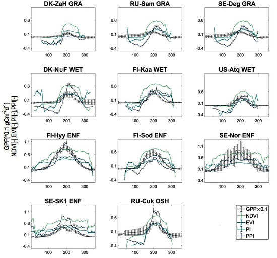
3.1. Seasonal Variations in Canopy Photosynthesis in Pan-Arctic Regions

The performances of the VIs such as NDVI, EVI, PI, and PPI to track canopy photosynthesis varied across different landscapes in the pan-Arctic (Figure 2). NDVI typically responded first, with EVI initiating a sharp increase after the leaves began to emerge. NDVI was always higher than the other indices during the growing season. PPI consistently followed the GPP curve compared with other indices across different plant functional types. PPI and PI started to increase 1 or 2 weeks later in most sites compared with the initial increase in GPP. This indicated that photosynthesis might start before the accumulation of photosynthetic biomass that could be measured by remote sensing optical sensors. NDVI differed substantially between the growing season and the snow season, but was less dynamic during the growing season, except for some possible noise-induced fluctuations. EVI produced a noise-free growing-season signal and was highly correlated with ground-observed phenology scores during the growing phase. However, EVI fluctuated during the winter, creating difficulties in identifying the growing season.

In wetland sites such as DK-NuF and US-Atq, EVI showed a declining trend before the biological recovery and an increasing trend after the growing season ended, while NDVI had a relatively better performance. In ENF sites where the seasonal dynamics were more obvious, NDVI also followed an increasing trend after the end of the growing season. Similar effects also seemed to apply to PPI in spring, as found in DK-NuF, FI-Sod, RU-Cok, SE-Sk1, and US-Atq, respectively.

For both NDVI and EVI, abnormal values around 0.35 appeared during the transition dates in non-growing seasons. These phenomena were significant for EVI in wetland tundra, with abnormal values up to 0.73. As for PI, the growing seasons indicated by the seasonal cycles seemed to be mismatched with the EC estimates. PI seemed to indicate longer growing seasons at SE-SK1 and SE-Nor, but shorter growing seasons at US-Atq and DK-ZaH. Notably, midsummer dips in NDVI and EVI in the middle of the growing season, also detected in other studies, were evident in some sites such as FI-Hyy, FI-Kaa, RU-Cok, SE-Deg, SE-Nor, and SE-SK1, respectively.

The EC sites of FI-Sod, RU-Cok, DK-NuF, and DK-ZaH represented ENF, OSH, WET, and GRA, ecosystems, respectively, with relatively long-term observations (Figure 3). The indices showed similar but different characteristics of inter-annual dynamics across different landscapes. Most indices tended to follow the time dynamics of the phenology indicated by the GPP time series. However, the start and end of measurable photosynthesis were difficult to capture and varied inter-annually. In WET sites like DK-NuF in the pan-Arctic tundra, EVI largely failed to track the inter-annual dynamics, while NDVI, PI, and PPI showed close relationships between inter-annual variations and EC estimates for ENF, OSH, and WET, and thus tracked vegetation phenology. PI might prove useful for deciduous broadleaf forests (DBF) sites, however, the implementation of objective functions to extract SOS and EOS was challenging. Of all the curves, PPI showed relatively larger dynamics during the growing season and followed the inter-annual ground data best, with the fewest abnormal values.

3.2. Phenology Metrics Estimated by Different VIs

The performance of estimations extracted by VIs varies across different ecosystems. The estimated SOS and EOS were comparable but not equivalent (Figure 4). Considerable variations were found in the phenology transitions dates. In terms of GPP (as the reference), we found a difference of 74 days between the average phenological transition dates of the four landscapes for SOS, and a difference of 41 days for EOS. Generally, EVI-extracted phenological transition dates seemed to lengthen the season, by contrast, MCD12 and PI seemed to indicate a relatively short seasonal duration. PPI was more robust in phenology extraction especially at the beginning of the growing season.

In WET sites in Greenland and northern Europe, the dormancy onset of photosynthesis occurred generally around day 256 according to the EC tower estimates. All of the MODIS estimations seemed to postpone the autumn abscission. Furthermore, both NDVI and EVI indicated longer growing seasons, around day 287 and day 282 respectively, while PPI indicated a similar length of the season. In GRA sites, PI showed a similar SOS but failed to track EOS by postponing the autumn abscission by 11 days, while NDVI and MCD12 shortened the growing season by an average of 10 days and 43 days, respectively. In the OSH site, all the MODIS-based indices tracked the tower-based onset reasonably well, and the variations between SOS and EOS extracted by the different indices were relatively small. Nevertheless, photosynthesis onset based on MODIS PPI were relatively closer to the tower data. Regarding ENF sites, the onset of photosynthesis according to the tower-based data occurred between about days of 70 and 119. The multi-model mean values generally showed a similar, later onset of photosynthesis, except in the case of EVI with the lowest value of day 41.

SOS and EOS dates based on all the indices correlated significantly (p < 0.05) with GPP estimations, indicating that remote sensing and in situ phenology dates responded to the same climate variables, but responded differently. Estimates of SOS and EOS in sites with different vegetation types derived using the same fitting function varied according to the different functional plant types, but most had relatively low R² values (

Table A3. SOS and EOS across different landscapes in the pan-Arctic. The comparison is done with GPP. RMSE stands for root-mean-square error.

Metrics	LC	Indices	R2	Equation	RMSE
SOS	GRA	NDVI	0.31	y = 0.68x + 31.59	94
		EVI	0.41	y = 0.47x + 84.959	41.02
		PI	0.04	y = 0.16x + 92	76.32
		PPI	0.03	y = 0.21x +105.7	33.17
		MCD12	0.4	y = 0.99x − 19.16	20
	WET	NDVI	0.43	y = 0.58x + 64.06	10.4
		EVI	0.1	y = 0.2379x + 116.09	59.02
		PI	0.27	y = 0.394x + 85.857	50.44
		PPI	0.004	y = −0.02x + 151.8	14.01
		MCD12	0.06	y = −0.19x + 176.2	15.44
	ENF	NDVI	0.17	y = 0.24x + 68.29	81.6
		EVI	0.3	y = −0.12x + 112.17	12.78
		PI	0.15	y = 0.27x + 64.21	83.54
		PPI	0.07	y = 0.2x + 68.91	18.27
		MCD12	0.22	y = 0.62x + 16.11	16.75
	OSH	NDVI	0.6	y = -1.93x + 455.3	8.353
		EVI	0.13	y = −0.29x + 200	13.42
		PI	0.06	y = −0.39x + 218.1	14.97
		PPI	0.08	y = 0.25x + 118.6	13.87
		MCD12	0.04	y = −0.29x + 209.3	11.95
EOS	GRA	NDVI	0.19	y = 0.41x + 155.8	32.81
		EVI	0.11	y = 0.25x + 199.5	54.31
		PI	0.11	y = 0.17x + 229.06	38.89
		PPI	0.01	y = −0.07x + 290.5	20.35
		MCD12	0.14	y = 0.54x + 133.1	22.16
	WET	NDVI	0.03	y = −0.10x + 291.67	91.9
		EVI	0.09	y = 0.18x + 206.6	77.25
		PI	0.36	y = 0.31x + 177.66	32.72
		PPI	0.02	y = −0.06x + 275.6	11.99
		MCD12	0.13	y = 0.25x + 193.7	11.49
	ENF	NDVI	0.24	y = −0.23x + 357.75	9.07
		EVI	0.08	y = −0.13x + 324.9	55.48
		PI	0.28	y = −0.20x + 349.16	6.99
		PPI	0.04	y = −0.08x + 313.5	12.4
		MCD12	0.09	y = 0.23x + 232.1	14.2
	OSH	NDVI	0.09	y = 0.4x + 155.2	14.4
		EVI	0.01	y = 0.03x + 255.3	14.9
		PI	0.11	y = 0.16x + 221.8	13.73
		PPI	0.68	y = 0.43x + 157.5	7.73
		MCD12	0.04	y = −0.37x + 358.2	13.77

). There were substantial differences in the performances of the five indices for predicting SOS across the array of functional plant types included in the study. None of the five indices provided reliable SOS estimates in OSH sites (Figure 5). The SOS in GRA sites was better modeled, with all approaches yielding SOS estimates that were significantly correlated with tower-based observations (R² = 0.03–0.41). The correlation between all four indices and GPP in ENF sites was quite low (R² = 0.07–0.22), but NDVI performed better in WET sites (R² = 0.43, RMSE = 10.4).

For EOS, the relationships between GPP-based and remotely sensed estimates were also significant (p < 0.05), but less significant than for SOS, suggesting that the autumn VI values could not provide an accurate indicator of the timing of leaf defoliation. EVI and PPI provided the lowest R² (R² = 0.01, p < 0.005), while NDVI showed the highest RMSE compared with GPP-based EOS. Compared with SOS, all models predicting observed EOS performed comparably for a given functional type (Figure 5). NDVI performed better in GRA sites, though R² was low (0.19), while all methods predicting EOS in WET sites were significantly correlated with observations, with modest differences in the strength of the correlation (R² = 0.02–0.36). The coefficients between SOS dates extracted from VIs in ENF sites and tower-observed GPP were all below 0 except MCD12 (R² = 0.09 RMSE = 14.2). Interestingly, although PPI was more robust and fitted GPP more closely, as discussed above (Figure 2), its performance for the extraction of SOS and EOS was not generally significantly better. PPI EOS estimates matched GPP better than any other method in our study, with the highest R² of 0.68 and the lowest RMSE of 7.73, yet the comparable numbers for PPI SOS were miserable (R² = 0.08 RMSE = 13.87).

4. Discussion

4.1. Comparison of Different Vegetation Phenology Indices

An improved ability to describe the timing of phenological transitions accurately is crucial for a better understanding of climate–ecosystem linkages under current circumstances, especially in pan-Arctic regions. Our current results highlighted the existence of relationships between remotely sensed and GPP based estimations of phenological metrics, but these were inconsistent among the different indices.

Our results showed that NDVI experienced abrupt variations at the beginning and end of the snow seasons indicating that NDVI is more sensitive than EVI and PI to snow at low fractional snow cover (Figure 6). The results also revealed a large gap between NDVI and EVI during the non-growing season, which can be explained as EVI is more sensitive to fractional snow variation at high snow coverage [50]. EVI and NDVI had stationary phases in the middle of the growing season. Unlike the saturation effects in high-biomass areas, which could be attributed to the increased contrast of the reflectances of the NIR and red band caused by non-linear stretching [47], the stationary phases of NDVI and EVI in the mid-growing season were caused by unstable fluctuations. In general, the most commonly used VI, NDVI, did not provide an ideal measurement of GPP in pan-Arctic regions, especially in ENF regions. EVI also showed large uncertainties at the onset of spring since it was strongly affected by the snow filtering and hard to predict the snow gone stages precisely [53]. Compared with EVI, MCD12 always shortened the growing season (Figure 4). In GRA, WET and ENF sites, for both SOS and EOS, MCD12 and EVI had comparable R² but MCD12 had less the RMSE in different extents (Table A3). In the OSH site, both of them had comparably poor R² (<0.13) and RMSE (>11.95). The general pattern showed that MCD12 usually did a better job in terms of RMSE than our retrievals, indicating the additional levels of quality control and filtering result in a more consistent product, even if it is a not very accurate indicator of flux tower data.

In our study at higher latitudes, PI only improved phenology extraction in some sites (FI-Hyy, FI-Kaa, FI-Sod, and US-Atq) compared with traditional VIs, particularly at the onset of spring. Although PI showed a smoother time series, it was not an ideal index for extracting SOS and EOS in pan-Arctic regions [4].

PPI-based phenology retrieval of transition dates showed improved performance compared with traditional VIs. First, PPI was more robust, and more valid data on phenological transition dates could be extracted from PPI compared with the other indices in this study over the same time period. Second, PPI had fewer occurrences of negative R values compared with the other indices, except in ENF sites. In ENF sites, almost all of the phenological transition dates extracted by satellite observations showed relatively low correlations with tower-based GPP. PPI was able to detect the timings of SOS and EOS more precisely when evaluated against ground-observed GPP data in OSH sites. We found a surprisingly strong relationship between MODIS-based PPI SOS and GPP-based SOS (R² = 0.68, RMSE = 7.73). Other studies in the northern hemisphere Boreal Zone also suggested improved performance of PPI over NDVI and EVI for the retrieval of SOS [54]. Modeling and satellite observations showed that the influence of snow on PPI was less severe than on the traditional vegetation indices. However, because the red reflectance of soil and vegetation may differ greatly, PPI is more sensitive to soil brightness than EVI, though the difference is reduced with increasing LAI [50].

We demonstrated a clear systematic difference between VIs, likely related to their different sensitivities to changes in snow cover and vegetation activity. Remote sensing VIs were more closely related to the development of the canopy structure, which occurred ahead of photosynthesis in the spring and persisted after the cessation of photosynthesis in the autumn. It was therefore difficult to use a single VI to estimate phenology for pan-Arctic vegetation due to the limitations of background reflectance.

4.2. Phenological Transitions in Different Landscapes

The different sensitivities of the indices to phenological transitions were likely due to the reflectance at each pixel, which was the result of a variety of vegetation and background features [55]. Different landscapes also impacted the performances of tracking SOS and EOS differently. Our results may thus have important implications for the usefulness and limitations of different VIs for extracting SOS and EOS from various biomes.

For ecosystems with greater seasonal variations in greenness (e.g., GRA, WET, and OSH sites), at least one index produced estimates that agreed better with EC estimations, though the correlations were still not very high. The current SOS and EOS clearly showed that the land surface phenology extracted from the traditional vegetation indices were poorly correlated with EC-estimated GPP in ENF sites, which could be attributed to the fact that seasonal changes in evergreen plants have little effect on the spectral information. The water contained in live vegetation in early spring and late autumn masks the trend of VIs in needleleaf forests. The timing of the actual growing season was therefore likely to be earlier than that indicated by remote sensing methods, and photosynthesis in ENF areas may last until the end of the growing season. A recent study has shown chlorophyll/carotenoid index (CCI) could better monitor photosynthesis of ENF from optical remote sensing by using the combination of MODIS band 1 and band 11 [56]. Nevertheless, remotely sensed estimates in pan-Arctic regions need to be interpreted with appropriate guidance. And the validations of phenological metrics estimated by satellite data are necessary before it can be meaningfully interpreted.

4.3. Future Prospects for Capturing Phenology Metrics in Pan-Arctic regions

The ability to monitor phenology at a landscape scale is important to provide a better understanding of temporal and spatial phenology patterns in pan-Arctic ecosystems and their responses to climate change. Although remote sensing methods can deliver this scale of analysis, uncertainties over their use remain. The current results suggested that remotely sensed phenology and phenology derived from tower-based GPP were related, but with a low overall R value (−0.77 to 0.82). Here, we discussed the possible factors responsible for the highly varied and uncertain estimations. Remote sensing VIs more closely reflect structural canopy development. Systematic differences could be explained by the different responses of VIs to greenness, wetness, and brightness dynamics. The uncertainties were therefore mainly associated with several factors, as described below.

The main impact factor was background reflectance contamination due to factors such as snow, soil, soil thaw, and snow melt, which also had distinct seasonal dynamics. The presence of snow decreased NDVI values sharply due to changes in canopy background brightness, while values recovered when the snow melted in April [47]. Phenology metrics extracted from remote sensing VIs at high latitudes are known to be subject to background interference, largely due to snow cover. Although targeted snow flags and weighting schemes have been included in the pre-processing algorithms of some products, it remains difficult to distinguish soil and snow cover interference from vegetation phenology when the greenness signal from the vegetation is very weak. Previous studies acknowledged that snow cover had significant impacts on VIs [22,57,58]. Careful data screening and pre-processing are therefore needed to eliminate the impact of snow [59]. Another possible source of uncertainty in the estimations of SOS and EOS from the different indices could be attributed to the extraction method. The rise of NDVI at the start of spring was generally more abrupt than the end of spring, meaning the fitted VIs may slightly overestimated the values before the start of spring while underestimating the values at the start of spring [30] . Other methods such as a threshold method or other fitting functions have also commonly been used. However outputs using data acquired from MODIS tended to give earlier SOS and EOS dates compared with in situ observations in other commonly used approaches [23].

To illustrate the influence of snow, NDSI was computed from MODIS surface reflectance product MCD43A4 C5 (Figure 6). In both sites of FI-Hyy and SE-Deg, opposite variations tendency of NDVI and NDSI occurred suggesting that NDVI might be influenced by snow melt. Large fluctuations were found in the NDVI before the start and after the end of the growing season. EVI and PI seemed to be hindered by similar but weaker effects of snow melt. Meanwhile, there were large jumps in the EVI in deep winter. Conversely, those effects did not appear on PPI.

Other than the background reflectance contamination, there were other contributors to the limitations of LSP estimates in pan-Arctic regions. First, optical remote sensing methods are subject to atmospheric influences including atmospheric noise [60] and persistent cloud cover [61], low viewing angles, and low solar zenith angles. Second, the frequency of data sampling was 8 days over a 16-day period for the MODIS reflectance product, which meant that bud burst occurring within the 8-day periods was difficult to detect. Moreover, site-specific conditions were also a source of uncertainty, such as the pronounced spatial heterogeneity of pixels caused by the sparse vegetation [62]. Sites with relatively short growing seasons with few good-quality observations would make it even harder to extract the seasonal cycles.

Efforts were made to distinguish the effective greening up of spring from snow melt such as developing new methods including winter NDVI, which is the NDVI outside the growing season, in monitoring vegetation activities in deciduous and ever green forest in northern Scandinavia [30]. Another possible solution would be including more newly released MODIS reflectance product Collection 6 (C6). A recent study found that, in the Tibetan Plateau, NDVI from Collection 5 (C5) SOS was more consistent than C6 SOS in terms of ground-observed green-up dates for alpine grassland [63]. Although there was improved quality at high latitudes from use of all available observations in C6 than C5 who used only four observations per day. The results showed there was no significant improvement for C6 in extracting phenological metrics (

Table 2. SOS and EOS extracted by MODIS reflectance product Collection 5 and Collection 6 at FI-Hyy. The comparison is done with GPP. RMSE stands for root-mean-square error.

		Collection 6		Collection 5
Metrics	Indices	R2	RMSE	R2	RMSE
SOS	NDVI	0.001	10.73	0.38	7.68
	EVI	0.39	9.392	0.09	12.54
	PI	0.08	9.705	0.14	8.08
	PPI	0.14	8.175	0.2	8.14
EOS	NDVI	0.02	18.37	0.23	19.34
	EVI	0.07	19.07	0.1	17.78
	PI	0.08	17.91	0.01	15.87
	PPI	0.03	16.11	0.14	14.35

), suggesting that the use of C6 may not help tackle the influence of snow, soil moisture on estimates of phenological metrics. However, further study is still needed.

Alternatively, after the first retrievals of chlorophyll fluorescence from satellite measurements on a global scale [64], strong correlations were found between tower-based GPP and satellite-derived SIF. Chlorophyll absorbs photons to provide energy for photosynthesis, and some photons are then released at longer wavelengths in the form of fluorescence. A recent study found that canopy-level SIF retained a strong linear correlation with GPP in deciduous forests (R² = 0.82) [65]. However, correlations between SIF and GPP are affected by factors such as wavelength, biomass, ecosystem, canopy structure, and timescale [66].

We tested if SIF could capture the phenological transition dates of ENF in pan-Arctic regions. In relatively homogeneous ENF EC sites in pan-Arctic regions, SIF and tower-based GPP showed similar seasonal cycles in highly homogenous EC sites (Figure 7). Both SIF and EC based GPP also indicated the onset of photosynthetic activity in early April. The high correlation in annual dynamic changes suggested that SIF could be used as a phenology indicator in pan-Arctic regions. SIF was more closely related to GPP in ENF sites than in OSH sites. This could be explained by the fact that the carbon sequestration capacity of the OSH itself was not very strong, as well as by noise during the non-growing season and errors caused by the remote sensing algorithm.

In ENF sites, the relationship between SIF-based and GPP-based estimates was significant for both SOS and EOS (p < 0.05). SIF-based SOS demonstrated a better relationship with GPP (R² = 0.34; Figure 8), whereas NDVI performed best among the four indices, although with relatively low R² (R² = 0.17; Table A3).

Satellite chlorophyll fluorescence has shown potential for improving the accuracy of monitoring phenology at a global scale. It can be used to track the onset of spring and the end of the season in forest ecosystems [20], while the VI and models based on reflectance often overestimate the length of the photosynthetic cycle. SIF could lead to an improved assessment of photosynthetic phenology, particularly for evergreen coniferous forests that have been difficult to measure from satellites using more conventional vegetation indices. In pan-Arctic regions where the influence of snow, soil moisture, and other factors are relatively large, the development of advanced instruments such as OCO-2 [67,68] suggests that SIF may play a more important role in monitoring phenology. To better estimate the phenological metrics in pan-Arctic regions, other possibilities would be combining vegetation indices and indices that illustrate the information of snow or soil moisture (e.g. NDWI and NDSI). Or to take into account spatio-temporal variations of soil moisture through monitoring with SAR data [69].

5. Conclusions

This study analyzed the reliability of various MODIS-derived indices and SIF for estimating phenological transition dates in pan-Arctic regions, and reported a high level of uncertainty regarding phenology extraction at these latitudes. The results indicated that all indices were influenced by snow cover and soil moisture during the transition dates, and although VI-based and EC-based estimates of phenological transition dates were related, the overall R² values were low. Available methods for satellite-derived time series in pan-Arctic regions were mainly constrained by constant snow cover, solar geometry, site-specific conditions, the short length of the growing season, and the relatively low frequency of data sampling. Of the tested VIs, PPI-estimated metrics showed seasonal and inter-annual patterns that were mostly closely related to the EC-based estimates. SIF was also shown to be a suitable indicator of the SOS and EOS in pan-Arctic regions, and may play an increasingly important role in line with advances in instrumentation.

The results of this study challenge the utility of satellite-derived VIs for assessing phenology and its changes in high-latitude regions, given that estimates of phenological transition dates based on optical remote sensing are likely to coincide with the disappearance of snow, unless careful data screening and pre-processing are carried out to avoid this impact. Precautions must therefore be taken when interpreting spatio-temporal patterns of SOS derived from these indices. Significantly, careful validation with ground data are required for critical regions to enable the reliable detection of changes and to further our understanding of ecosystems to the level needed to allow accurate predictions to be made.

References

1. Peñuelas, J.; Filella, I. Phenology feedbacks on climate change. Science 2009, 324, 887–888. [Google Scholar] [CrossRef] [PubMed] [Green Version]
2. Keenan, T.F. Phenology: Spring greening in a warming world. Nature 2015, 526, 48–49. [Google Scholar] [CrossRef] [PubMed]
3. Hogda, K.A.; Tommervik, H.; Karlsen, S.R. Trends in the Start of the Growing Season in Fennoscandia 1982–2011. Remote. Sens. 2013, 5, 4304–4318. [Google Scholar] [CrossRef] [Green Version]
4. Gonsamo, A.; Chen, J.M.; Price, D.T.; Kurz, W.A.; Wu, C. Land surface phenology from optical satellite measurement and CO2eddy covariance technique. J. Geophys. Res. Biogeosci. 2012, 117. [Google Scholar] [CrossRef] [Green Version]
5. Gonsamo, A.; Chen, J.M. Circumpolar vegetation dynamics product for global change study. Remote. Sens. Environ. 2016, 182, 13–26. [Google Scholar] [CrossRef] [Green Version]
6. Tang, J.; Körner, C.; Muraoka, H.; Piao, S.; Shen, M.; Thackeray, S.J.; Yang, X. Emerging opportunities and challenges in phenology: A review. Ecosphere 2016, 7, e01436. [Google Scholar] [CrossRef]
7. Richardson, A.D.; Hufkens, K.; Milliman, T.; Frolking, S. Intercomparison of phenological transition dates derived from the PhenoCam Dataset V1.0 and MODIS satellite remote sensing. Sci. Rep. 2018, 8, 5679. [Google Scholar] [CrossRef] [PubMed]
8. D’Odorico, P.; Gonsamo, A.; Gough, C.M.; Bohrer, G.; Morison, J.; Wilkinson, M.; Hanson, P.J.; Gianelle, D.; Fuentes, J.D.; Buchmann, N. The match and mismatch between photosynthesis and land surface phenology of deciduous forests. Agric. For. Meteorol. 2015, 214–215, 25–38. [Google Scholar] [CrossRef]
9. Henebry, G.M.; de Beurs, K.M. Remote Sensing of Land Surface Phenology: A Prospectus; Springer: Dordrecht, The Netherlands, 2013. [Google Scholar]
10. Zhang, X.; Wang, J.; Gao, F.; Liu, Y.; Schaaf, C.; Friedl, M.; Yu, Y.; Jayavelu, S.; Gray, J.; Liu, L.; et al. Exploration of scaling effects on coarse resolution land surface phenology. Remote. Sens. Environ. 2017, 190, 318–330. [Google Scholar] [CrossRef]
11. Richardson, A.D.; Black, T.A.; Ciais, P.; Delbart, N.; Friedl, M.A.; Gobron, N.; Hollinger, D.Y.; Kutsch, W.L.; Longdoz, B.; Luyssaert, S. Influence of spring and autumn phenological transitions on forest ecosystem productivity. Philos. Trans. Boil. Sci. 2010, 365, 3227–3246. [Google Scholar] [CrossRef] [PubMed] [Green Version]
12. Garrity, S.R.; Bohrer, G.; Maurer, K.D.; Mueller, K.L.; Vogel, C.S.; Curtis, P.S. A comparison of multiple phenology data sources for estimating seasonal transitions in deciduous forest carbon exchange. Agric. For. Meteorol. 2011, 151, 1741–1752. [Google Scholar] [CrossRef]
13. Noormets, A.; Chen, J.; Gu, L.; Desai, A. The Phenology of Gross Ecosystem Productivity and Ecosystem Respiration in Temperate Hardwood and Conifer Chronosequences. In Phenology of Ecosystem Processes: Applications in Global Change Research; Noormets, A., Ed.; Springer: New York, NY, USA, 2009; pp. 59–85. [Google Scholar]
14. White, K.; Pontius, J.; Schaberg, P. Remote sensing of spring phenology in northeastern forests: A comparison of methods, field metrics and sources of uncertainty. Remote. Sens. Environ. 2014, 148, 97–107. [Google Scholar] [CrossRef]
15. Zhang, Y.; Zhu, Z.; Liu, Z.; Zeng, Z.; Ciais, P.; Huang, M.; Liu, Y.; Piao, S. Seasonal and interannual changes in vegetation activity of tropical forests in Southeast Asia. Agric. For. Meteorol. 2016, 224, 1–10. [Google Scholar] [CrossRef]
16. Luo, X.; Chen, X.; Wang, L.; Xu, L.; Tian, Y. Modeling and predicting spring land surface phenology of the deciduous broadleaf forest in northern China. Agric. For. Meteorol. 2014, 198–199, 33–41. [Google Scholar] [CrossRef]
17. Richardson, A.D.; Keenan, T.F.; Migliavacca, M.; Ryu, Y.; Sonnentag, O.; Toomey, M. Climate change, phenology, and phenological control of vegetation feedbacks to the climate system. Agric. For. Meteorol. 2013, 169, 156–173. [Google Scholar] [CrossRef]
18. Joiner, J.; Yoshida, Y.; Vasilkov, A.P.; Schaefer, K.; Jung, M.; Guanter, L.; Zhang, Y.; Garrity, S.; Middleton, E.M.; Huemmrich, K.F.; et al. The seasonal cycle of satellite chlorophyll fluorescence observations and its relationship to vegetation phenology and ecosystem atmosphere carbon exchange. Remote. Sens. Environ. 2014, 152, 375–391. [Google Scholar] [CrossRef] [Green Version]
19. Walther, S.; Voigt, M.; Thum, T.; Gonsamo, A.; Zhang, Y.; Kohler, P.; Jung, M.; Varlagin, A.; Guanter, L. Satellite chlorophyll fluorescence measurements reveal large-scale decoupling of photosynthesis and greenness dynamics in boreal evergreen forests. Glob. Chang. Boil. 2016, 22, 2979–2996. [Google Scholar] [CrossRef] [PubMed] [Green Version]
20. Lu, X.; Cheng, X.; Li, X.; Chen, J.; Sun, M.; Ji, M.; He, H.; Wang, S.; Li, S.; Tang, J. Seasonal patterns of canopy photosynthesis captured by remotely sensed sun-induced fluorescence and vegetation indexes in mid-to-high latitude forests: A cross-platform comparison. Sci. Total. Environ. 2018, 644, 439–451. [Google Scholar] [CrossRef] [PubMed]
21. Huete, A.R. A soil-adjusted vegetation index (SAVI). Remote Sensing of Environment. Remote. Sens. Environ. 1988, 25, 295–309. [Google Scholar] [CrossRef]
22. Nagai, S.; Nasahara, K.N.; Muraoka, H.; Akiyama, T.; Tsuchida, S. Field experiments to test the use of the normalized-difference vegetation index for phenology detection. Agric. For. Meteorol. 2010, 150, 152–160. [Google Scholar] [CrossRef] [Green Version]
23. Wu, C.; Peng, D.; Soudani, K.; Siebicke, L.; Gough, C.M.; Arain, M.A.; Bohrer, G.; Lafleur, P.M.; Peichl, M.; Gonsamo, A.; et al. Land surface phenology derived from normalized difference vegetation index (NDVI) at global FLUXNET sites. Agric. For. Meteorol. 2017, 233, 171–182. [Google Scholar] [CrossRef]
24. Luo, X.; Chen, X.; Xu, L.; Myneni, R.; Zhu, Z. Assessing Performance of NDVI and NDVI3g in Monitoring LeafUnfolding Dates of the Deciduous Broadleaf Forest in Northern China. Remote. Sens. 2013, 5, 845–861. [Google Scholar] [CrossRef]
25. Rees, W.G.; Golubeva, E.I.; Williams, M. Are vegetation indices useful in the Arctic? Pol. Rec. 2009, 34, 333. [Google Scholar] [CrossRef]
26. Luus, K.A.; Commane, R.; Parazoo, N.C.; Benmergui, J.; Euskirchen, E.S.; Frankenberg, C.; Joiner, J.; Lindaas, J.; Miller, C.E.; Oechel, W.C.; et al. Tundra photosynthesis captured by satellite-observed solar-induced chlorophyll fluorescence. Geophys. Res. Lett. 2017, 44, 1564–1573. [Google Scholar] [CrossRef] [Green Version]
27. Chen, J.; Jönsson, P.; Tamura, M.; Gu, Z.; Matsushita, B.; Eklundh, L. A simple method for reconstructing a high-quality NDVI time-series data set based on the Savitzky–Golay filter. Remote. Sens. Environ. 2004, 91, 332–344. [Google Scholar] [CrossRef]
28. Elmore, A.J.; Guinn, S.M.; Minsley, B.J.; Richardson, A.D. Landscape controls on the timing of spring, autumn, and growing season length in mid-Atlantic forests. Glob. Chang. Boil. 2012, 18, 656–674. [Google Scholar] [CrossRef]
29. Gonsamo, A.; Chen, J.M.; D’Odorico, P. Deriving land surface phenology indicators from CO2 eddy covariance measurements. Ecol. Indic. 2013, 29, 203–207. [Google Scholar] [CrossRef]
30. Beck, P.S.A.; Atzberger, C.; Høgda, K.A.; Johansen, B.; Skidmore, A.K. Improved monitoring of vegetation dynamics at very high latitudes: A new method using MODIS NDVI. Remote. Sens. Environ. 2006, 100, 321–334. [Google Scholar] [CrossRef]
31. Walker, M.A.; Fja, D.; Evander, M. Circumpolar arctic vegetation: Introduction and perspectives. J. Veg. Sci. 2010, 5, 757–764. [Google Scholar] [CrossRef]
32. Høye, T.T.; Post, E.; Schmidt, N.M.; Trøjelsgaard, K.; Forchhammer, M.C. Shorter flowering seasons and declining abundance of flower visitors in a warmer Arctic. Nat. Clim. Chang. 2013, 3, 759. [Google Scholar] [CrossRef]
33. Schimel, D.; Pavlick, R.; Fisher, J.B.; Asner, G.P.; Saatchi, S.; Townsend, P.; Miller, C.; Frankenberg, C.; Hibbard, K.; Cox, P. Observing terrestrial ecosystems and the carbon cycle from space. Glob. Chang. Boil. 2015, 21, 1762–1776. [Google Scholar] [CrossRef] [PubMed]
34. Walker, D.A.; Raynolds, M.K.; Einarsson, E.; Elvebakk, A.; Gould, W.A.; Talbot, S.S.; Yurtsev, B.A. The Circumpolar Arctic Vegetation Map. J. Veg. Sci. 2010, 16, 267–282. [Google Scholar] [CrossRef]
35. Lund, M.; Falk, J.M.; Friborg, T.; Mbufong, H.N.; Sigsgaard, C.; Soegaard, H.; Tamstorf, M.P. Trends in CO2 exchange in a high Arctic tundra heath, 2000–2010. J. Geophys. Res. Biogeosci. 2015, 117, 136. [Google Scholar]
36. Kutzbach, L.; Wille, C.; Pfeiffer, E.M. Heat, water and carbon exchange between arctic tundra and the atmospheric boundary layer - the eddy covariance method. Available online: http://epic.awi.de/11002/ (accessed on 20 October 2018).
37. Van der Molen, M.K.; Van Huissteden, J.; Parmentier, F.J.W.; Petrescu, A.M.R.; Dolman, A.J.; Maximov, T.C.; Kononov, A.V.; Karsanaev, S.V.; Suzdalov, D.A. The growing season greenhouse gas balance of a continental tundra site in the Indigirka lowlands, NE Siberia. Biogeosciences 2007, 4, 985–1003. [Google Scholar] [CrossRef] [Green Version]
38. Laurila, T.; Thum, T.; Aurela, M.; Lohila, A. Carbon Dioxide Fluxes between the Scots Pine Forest and the Atmosphere, Meteorology and Biomass Data during SIFLEX-2002; Final Report of SIFLEX-2002 Project; European Space Agency: Paris, France, 2003. [Google Scholar]
39. Westergaard-Nielsen, A.; Lund, M.; Hansen, B.U.; Tamstorf, M.P. Camera derived vegetation greenness index as proxy for gross primary production in a low Arctic wetland area. ISPRS J. Photogramm. Remote. Sens. 2013, 86, 89–99. [Google Scholar] [CrossRef]
40. Suni, T.; Rinne, J.; Reissell, A.; Altimir, N.; Keronen, P.; Rannik, Ü.; Dal Maso, M.; Kulmala, M.; Vesala, T. Long-term measurements of surface fluxes above a Scots pine forest in Hyytiälä, southern Finland, 1996–2001. Boreal Environ. Res. 2003, 8, 287–301. [Google Scholar]
41. Kolari, P.; Kuimaia, L.; Pumpanen, J.; Launiainen, S.; Ilvesniemi, H.; Han, P.; Nikinmaa, E. CO2 exchange and component CO2 fluxes of a boreal Scots pine forest. Boreal Environ. Res. 2009, 14, 761–783. [Google Scholar]
42. Aurela, M.; Laurila, T.; Tuovinen, J.P. Annual CO2 balance of a subarctic fen in northern Europe: Importance of the wintertime efflux. J. Geophys. Res. Atmos. 2002, 107, ACH–17. [Google Scholar] [CrossRef]
43. Peichl, M.; Öquist, M.; Ottosson Löfvenius, M.; Ilstedt, U.; Sagerfors, J.; Grelle, A.; Lindroth, A.; Nilsson, M.B. A 12-year record reveals pre-growing season temperature and water table level threshold effects on the net carbon dioxide exchange in a boreal fen. Environ. Res. Lett. 2014, 9, 055006. [Google Scholar] [CrossRef] [Green Version]
44. Nilsson, M.; Sagerfors, J.; Buffam, I.; Laudon, H.; Eriksson, T.; Grelle, A.; Klemedtsson, L.; Weslien, P.E.R.; Lindroth, A. Contemporary carbon accumulation in a boreal oligotrophic minerogenic mire—A significant sink after accounting for all C-fluxes. Glob. Chang. Boil. 2008, 14, 2317–2332. [Google Scholar] [CrossRef]
45. Lindroth, A.; Lagergren, F.; Aurela, M.; Bjarnadottir, B.; Christensen, T.; Dellwik, E.; Grelle, A.; Ibrom, A.; Johansson, T.; Lankreijer, H.; et al. Leaf area index is the principal scaling parameter for both gross photosynthesis and ecosystem respiration of Northern deciduous and coniferous forests. Tellus B 2008, 60, 129–142. [Google Scholar] [CrossRef]
46. Chen, B.; Coops, N.C.; Fu, D.; Margolis, H.A.; Amiro, B.D.; Black, T.A.; Arain, M.A.; Barr, A.G.; Bourque, C.P.A.; Flanagan, L.B.; et al. Characterizing spatial representativeness of flux tower eddy-covariance measurements across the Canadian Carbon Program Network using remote sensing and footprint analysis. Remote. Sens. Environ. 2012, 124, 742–755. [Google Scholar] [CrossRef]
47. Huete, A.; Didan, K.; Miura, T.; Rodriguez, E.P.; Gao, X.; Ferreira, L.G. Overview of the radiometric and biophysical performance of the MODIS vegetation indices. Remote. Sens. Environ. 2002, 83, 195–213. [Google Scholar] [CrossRef]
48. Delbart, N.; Kergoat, L.; Le Toan, T.; Lhermitte, J.; Picard, G. Determination of phenological dates in boreal regions using normalized difference water index. Remote. Sens. Environ. 2005, 97, 26–38. [Google Scholar] [CrossRef]
49. Delbart, N.; Toan, T.L.; Kergoat, L.; Fedotova, V. Remote sensing of spring phenology in boreal regions: A free of snow-effect method using NOAA-AVHRR and SPOT-VGT data (1982–2004). Remote. Sens. Environ. 2008, 101, 52–62. [Google Scholar] [CrossRef]
50. Jin, H.; Eklundh, L. A physically based vegetation index for improved monitoring of plant phenology. Remote. Sens. Environ. 2014, 152, 512–525. [Google Scholar] [CrossRef]
51. Salomonson, V.V.; Appel, I. Estimating fractional snow cover from MODIS using the normalized difference snow index. Remote. Sens. Environ. 2004, 89, 351–360. [Google Scholar] [CrossRef]
52. White, M.A.; De Beurs, K.M.; Didan, K.; Inouye, D.W.; Richardson, A.D.; Jensen, O.P.; O’Keefe, J.; Zhang, G.; Nemani, R.R.; van Leeuwen, W.J.D.; et al. Intercomparison, interpretation, and assessment of spring phenology in North America estimated from remote sensing for 1982–2006. Glob. Chang. Boil. 2009, 15, 2335–2359. [Google Scholar] [CrossRef]
53. Sekhon, N.S.; Hassan, Q.K.; Sleep, R.W. Evaluating potential of MODIS-based indices in determining “Snow Gone” stage over forest-dominant regions. Remote. Sens. 2010, 2, 1348–1363. [Google Scholar] [CrossRef]
54. Karkauskaite, P.; Tagesson, T.; Fensholt, R. Evaluation of the Plant Phenology Index (PPI), NDVI and EVI for Start-of-Season Trend Analysis of the Northern Hemisphere Boreal Zone. Remote. Sens. 2017, 9, 485. [Google Scholar] [CrossRef]
55. Reed, B.C.; Brown, J.F.; Vanderzee, D.; Loveland, T.R.; Merchant, J.W.; Ohlen, D.O. Measuring phenological variability from satellite imagery. J. Veg. Sci. 1994, 5, 703–714. [Google Scholar] [CrossRef]
56. Gamon, J.A.; Huemmrich, K.F.; Wong, C.Y.; Ensminger, I.; Garrity, S.; Hollinger, D.Y.; Noormets, A.; Penuelas, J. A remotely sensed pigment index reveals photosynthetic phenology in evergreen conifers. Proc. Natl. Acad. Sci. USA 2016, 113, 13087–13092. [Google Scholar] [CrossRef] [PubMed]
57. Dye, D.G.; Tucker, C.J. Seasonality and trends of snow-cover, vegetation index, and temperature in northern Eurasia. Geophys. Res. Lett. 2003, 30. [Google Scholar] [CrossRef] [Green Version]
58. Shabanov, N.V.; Zhou, L.; Knyazikhin, Y.; Myneni, R.B. Analysis of interannual changes in northern vegetation activity observed in AVHRR data from 1981 to 1994. IEEE Trans. Geosci. Remote. Sens. 2002, 40, 115–130. [Google Scholar] [CrossRef]
59. Beurs, K.M.D.; Wright, C.K.; Henebry, G.M. Dual scale trend analysis for evaluating climatic and anthropogenic effects on the vegetated land surface in Russia and Kazakhstan. Environ. Res. Lett. 2009, 4, 940–941. [Google Scholar] [CrossRef]
60. Hird, J.N.; McDermid, G.J. Noise reduction of NDVI time series: An empirical comparison of selected techniques. Remote. Sens. Environ. 2009, 113, 248–258. [Google Scholar] [CrossRef]
61. Eastman, R.; Warren, S.G. Arctic cloud changes from surface and satellite observations. J. Clim. 2009, 23, 4233–4242. [Google Scholar] [CrossRef]
62. Fletcher, B.J.; Gornall, J.L.; Poyatos, R.; Press, M.C.; Stoy, P.C.; Huntley, B.; Baxter, R.; Phoenix, G.K. Photosynthesis and productivity in heterogeneous arctic tundra: Consequences for ecosystem function of mixing vegetation types at stand edges. J. Ecol. 2012, 100, 441–451. [Google Scholar] [CrossRef] [Green Version]
63. Zheng, Z.; Zhu, W. Uncertainty of Remote Sensing Data in Monitoring Vegetation Phenology: A Comparison of MODIS C5 and C6 Vegetation Index Products on the Tibetan Plateau. Remote. Sens. 2017, 9, 1288. [Google Scholar] [CrossRef]
64. Joiner, J.; Yoshida, Y.; Vasilkov, A.P.; Yoshida, Y.; Corp, L.A.; Middleton, E.M. First observations of global and seasonal terrestrial chlorophyll fluorescence from space. Biogeosci. Discuss. 2011, 8, 637–651. [Google Scholar] [CrossRef] [Green Version]
65. Yang, X.; Tang, J.; Mustard, J.F.; Lee, J.E.; Rossini, M.; Joiner, J.; Munger, J.W.; Kornfeld, A.; Richardson, A.D. Solar-induced chlorophyll fluorescence that correlates with canopy photosynthesis on diurnal and seasonal scales in a temperate deciduous forest. Geophys. Res. Lett. 2015, 42, 2977–2987. [Google Scholar] [CrossRef] [Green Version]
66. Damm, A.; Guanter, L.; Paul-Limoges, E.; Van der Tol, C.; Hueni, A.; Buchmann, N.; Eugster, W.; Ammann, C.; Schaepman, M.E. Far-red sun-induced chlorophyll fluorescence shows ecosystem-specific relationships to gross primary production: An assessment based on observational and modeling approaches. Remote. Sens. Environ. 2015, 166, 91–105. [Google Scholar] [CrossRef]
67. Lu, X.; Cheng, X.; Li, X.; Tang, J. Opportunities and challenges of applications of satellite-derived sun-induced fluorescence at relatively high spatial resolution. Sci. Total. Environ. 2018, 619–620, 649–653. [Google Scholar] [CrossRef] [PubMed]
68. Li, X.; Xiao, J.; He, B.; Altaf Arain, M.; Beringer, J.; Desai, A.R.; Emmel, C.; Hollinger, D.Y.; Krasnova, A.; Mammarella, I.; et al. Solar-induced chlorophyll fluorescence is strongly correlated with terrestrial photosynthesis for a wide variety of biomes: First global analysis based on OCO-2 and flux tower observations. Glob. Chang. Boil. 2018. [Google Scholar] [CrossRef] [PubMed]
69. Collingwood, A.; Charbonneau, F.; Shang, C.; Treitz, P. Spatiotemporal Variability of Arctic Soil Moisture Detected from High-Resolution RADARSAT-2 SAR Data. Adv. Meteorol. 2018, 2018, 1–17. [Google Scholar] [CrossRef]
Figure 1. Spatial distributions of the 11 eddy covariance flux sites. Figure generated using a conformal projection center at the North Pole with ArcMap 10.3 (http://www.esri.com/).
Remotesensing 10 01784 g001
Figure 2. Averaged seasonal dynamics of NDVI, EVI, PI, and PPI compared with GPP across different landscapes in the pan-Arctic during 2000–2014. Error bars represent standard deviation of indices and GPP.
Remotesensing 10 01784 g002
Figure 3. Seasonal cycles of remotely sensed NDVI, EVI, PI, and PPI time series fitted with daily tower-based GPP for the years 2000–2014. Fits were based on double logistic functions of time. Values < −1 indicated fitted rather than original value.
Remotesensing 10 01784 g003
Figure 4. Box plots of SOS and EOS estimated from tower-based GPP and four remote sensing-derived VIs. The central mark represents the mean, the edges of the box are the 25th and 75th percentiles, and the whiskers extend to the most extreme data points not considered outliers. SOS and EOS indicate the start and end of the season, respectively.
Remotesensing 10 01784 g004
Figure 5. Relationships between MODIS estimations and flux-based estimations of phenology transition dates. Y-axes indicate SOS and EOS extracted from GPP data observed by the Flux sites, while X-axes indicate the day of year of the phenological transition extracted by the different indices.
Remotesensing 10 01784 g005
Figure 6. Averaged VI sensitivities to the variation of snow coverage in ENF site of FI-Hyy in Finland during 2000-2014 and in GRA site of SE-Deg in Sweden during 2001-2006. Pink solid line shows snow activity indicated by the NDSI.
Remotesensing 10 01784 g006
Figure 7. Seasonal cycles of tower-based GPP observations and SIF measurements from GOME-2 in three relatively spatially homogenous FLUX sites (FI-Sod, RU-Cok, and FI-Hyy), where the dominate plant function type accounted for 87.6%, 75.3%, and 73.3%, respectively
Remotesensing 10 01784 g007
Figure 8. Correlation between SOS and EOS extracted from tower-based GPP and satellite-based SIF. Dashed lines represent the 1:1 line and continuous lines are simple regression fit function.
Remotesensing 10 01784 g008