Article

A Novel Approach for the Detection of Developing Thunderstorm Cells

German Weather Service, Frankfurter Str. 135, 63067 Offenbach, Germany
*
Author to whom correspondence should be addressed.
Remote Sens. 2019, 11(4), 443; https://doi.org/10.3390/rs11040443
Submission received: 16 January 2019 / Revised: 14 February 2019 / Accepted: 18 February 2019 / Published: 21 February 2019
(This article belongs to the Special Issue Remote Sensing Methods and Applications for Traffic Meteorology)

Abstract

:
This study presents a novel approach for the early detection of developing thunderstorms. To date, methods for the detection of developing thunderstorms have usually relied on accurate Atmospheric Motion Vectors (AMVs) for the estimation of the cooling rates of convective clouds, which correspond to the updraft strengths of the cloud objects. In this study, we present a method for the estimation of the updraft strength that does not rely on AMVs. The updraft strength is derived directly from the satellite observations in the SEVIRI water vapor channels. For this purpose, the absolute value of the vector product of spatio-temporal gradients of the SEVIRI water vapor channels is calculated for each satellite pixel, referred to as Normalized Updraft Strength (NUS). The main idea of the concept is that vertical updraft leads to NUS values significantly above zero, whereas horizontal cloud movement leads to NUS values close to zero. Thus, NUS is a measure of the strength of the vertical updraft and can be applied to distinguish between advection and convection. The performance of the method has been investigated for two summer periods in 2016 and 2017 by validation with lightning data. Values of the Critical Success Index (CSI) of about 66% for 2016 and 60% for 2017 demonstrate the good performance of the method. The Probability of Detection (POD) values for the base case are 81.8% for 2016 and 89.2% for 2017, respectively. The corresponding False Alarm Ratio (FAR) values are 22.6% (2016) and 36.4% (2017), respectively. In summary, the method has the potential to reduce forecast lead time significantly and can be quite useful in regions without a well-maintained radar network.

Graphical Abstract

1. Introduction

Cumulonimbus clouds (Cbs), also referred to as thunderstorm clouds, are a dangerous weather phenomenon. Lightning, wind gusts and turbulence, and hail and heavy precipitation, associated with Cbs, result in serious damages and danger to life. Early and reliable prediction of Cbs is therefore essential for the initiation of appropriate protective measures, e.g., the selection of alternate flight routes for airplanes, the temporary closure of airports, or precautionary measures for outdoor activities.
The authors of [1] were some of the first to discuss the physics of satellite-based detection of Cbs. They found that the difference between the InfraRed (IR) window channel and the water vapor channel can be used to detect Cbs. The approach is used currently for the operational detection of Cbs, e.g., [2,3]. More recently, it has been shown that mature Cbs can be detected by satellites with relatively high POD and low FAR, if the brightness temperature difference method according to [1] is applied to two water vapor channels (7.3 μ m and 6.2 μ m) in combination with Numerical Weather Prediction (NWP) filtering [4].
Cbs originate from rapid vertical updraft of moist and warm air triggered by mountains, radiative heating, or cold fronts. The lifecycle of Cbs can be described in several stages, which are illustrated in Figure 1.
During the first stage, cumulus and towering cumulus clouds form. The next stage, the developing stage, is characterized by fast cooling of the cloud top resulting from a strong updraft. This strong updraft leads to significant friction between the cloud particles, which is a trigger for lightning, in particular in the mixed phase regions [5]. The early developing phase is also referred to as Convective Initialization (CI). The updraft continues until the cell reaches the mature stage and dissipation starts. Mature cells can be accompanied by overshooting tops.
Thus, the strong vertical updraft of the clouds is theoretically a good indicator of developing thunderstorms, and its reliable detection would allow an improvement in forecast lead times. If the movement of the cloud object were well known, then the strong vertical updraft could be inferred from the cooling rate, defined by the temporal change of the brightness temperatures of the cells (cloud objects) between two subsequent satellite images. This has motivated several authors to use the temporal change of the brightness temperatures as essential interest fields (indicators) for the detection of convective initiation/developing thunderstorms, e.g., [6,7,8,9,10]. However, the movement of the cells between two subsequent satellite images needs to be known well in order to derive the cooling rate accurately. In other words, accurate meso-scale Atmospheric Motion Vectors (AMV) are required. Yet, this poses a serious challenge as, e.g., discussed in [11]. The basic problem of AMV methods is that they are under-determined. Convective cloud movement is a meso-scale 3D phenomenon, but only 2D satellite images are available for the detection of AMVs. Thus, all approaches that use AMV or Cloud Motion Vectors (CMV) need to deal with this under-determination. Consequently, convection typically leads to serious errors in the AMV; see, e.g., [11,12]. Further, smoothing and filtering by quality procedures hamper the accurate detection of the relevant meso-scale movement; see [11] for further details. The above-mentioned effects result in a serious amount of missed detections and false alarms. This in turn constitutes a serious handicap for operational usage.
For this reason, an alternative approach is discussed and evaluated in this study. This approach does not rely on atmospheric motion vectors, but the updraft strength is directly derived from the measurements in the water vapor channels of the Spinning Enhanced Visible and InfraRed Imager (SEVIRI) instrument on-board MSG [13]. For this purpose, the absolute value of the vector product of spatio-temporal gradients of the SEVIRI water vapor channels is calculated for each satellite pixel, referred to as the Normalized Updraft Strength (NUS). Spatial gradients mark regions with strong variations in water vapor temperatures, such as clouds punching through the water vapor layer. Combining these spatial gradients with a temporal gradient for a given location separates growing/cooling clouds from advected clouds. The main idea of the approach is that the vertical updraft of convective cells leads to NUS values significantly above zero, whereas horizontal cloud movement leads to NUS values close to zero. Thus, NUS is a measure of the vertical updraft strength and can be applied to distinguish between advection and convection. Thus, the updraft strength can be derived without the need for the atmospheric motion vectors; rather, the vertical movement is directly deduced from the satellite observations of the WV7.3 and WV6.2 channel. This breaks the problem down to the generation of 1D information from 2D information, aiming to resolve the problem of under-determination associated with classical atmospheric motion vector approaches.
The authors are not aware of any similar approach applied so far for the detection of the vertical updraft strength. Thus, we believe that we are presenting a novel approach, which will be of benefit to improve the detection of developing thunderstorms. Further, as the approach does not rely on AMVs, the implementation and operational maintenance are straightforward.
The term convective initialization is not well suited for validation purposes in consideration of the large satellite pixel size. Thus, we prefer the term developing thunderstorms. This means that the cells are still growing and have not yet reached maturity in terms of brightness temperature differences of the water vapor channels. This issue will be further discussed in Section 4.
The aim of this manuscript is the presentation and validation of a novel approach that is intended for operational 24/7 severe weather warnings covering Europe and Africa. For this purpose, we need a reliable operational data source. Therefore, the SEVIRI instrument on board the operational prime Meteosat satellite operating at a 0.0 degree geostationary orbit is used. The prime operational service provides data with a 15-min time resolution. SEVIRI comes with 12 channels, of which two cover the H 2 O emissivity bands in the IR. The spatial resolution is a 3 × 3 km sub-satellite point. Further details of the instrument can be found in [13].
Observational data play a pivotal role for the accurate detection and short-term forecast of developing thunderstorms due to the shortcomings of NWP models. Over oceans and a vast number of countries that are not well equipped with precipitation radars, satellites are the only observational source for the detection of developing thunderstorms; see, e.g., [14]. Furthermore, dry thunderstorms, which are a serious source of wildfires [15], cannot be detected with weather radars.

2. Materials and Methods

2.1. Method

The brightness temperatures of the water vapor channels of the SEVIRI instrument on board the Meteosat Second Generation satellites (MSG) were used for the calculation of the updraft strength of convective cells.
The satellite brightness temperatures were derived from the level 1.5 rectified image data of digital counts by application of the EUMETSAT calibration coefficients and conversion method. More detailed information on MSG and the SEVIRI instrument are given in [13].
The potential of the WV channel for Cb detection was first discussed in [1] and adapted to 2 water vapor channels by, e.g., [4]. Here, we present a novel approach for the detection of developing thunderstorms. The signal received by the satellite consists of the radiation emitted by the cloud top and the clear sky radiation above the cloud top. This is of relevance for the interpretation of the approach. The different channels and their clear sky weighting functions are shown in Figure 2.
In our approach, the absolute value of the vector product of spatio-temporal gradients of the SEVIRI water vapor channels was calculated for each satellite pixel, referred to as NUS. NUS is postulated to be a measure of the strength of the vertical updraft and used to distinguish between advection and convection. The calculation of NUS is described below. A 3-component vector is first generated from each of the 2 water vapor channels WV7.3 (7.3 μ m) and WV6.3 (6.3 μ m). The components of the vectors are defined as follows. The temporal change of the spatial brightness temperature gradients in the x and y direction of the WV7.3 and WV6.2 channel represent the x and y components of the vectors. The temporal change of the brightness temperatures at the pixel level represents the z components of the vectors. In order to deduce the temporal change information, two subsequent satellite images are used. The respective components are finally normalized by division of the BT in degrees Celsius of the respective channel. Please see Equations (1) and (2) for the mathematical description of the vector components of vbtf 7.3 and vbtf 6.2 . The components of the vectors might be interpreted as virtual brightness temperature fluxes (vbtf).
v b t f x , 7.3 = δ δ t δ x ( B T 7.3 ( t , x , y ) / ( B T 7.3 ( t o , x , y ) - 273 K ) v b t f y , 7.3 = δ δ t δ y ( B T 7.3 ( t , x , y ) / ( B T 7.3 ( t o , x , y ) - 273 K ) v b t f z , 7.3 = δ δ t ( B T 7.3 ( t , x , y ) / ( B T 7.3 ( t o , x , y ) - 273 K )
v b t f x , 6.2 = δ δ t δ x ( B T 6.2 ( t , x , y ) / ( B T 6.2 ( t o , x , y ) - 273 K ) v b t f y , 6.2 = δ δ t δ y ( B T 6.2 ( t , x , y ) / ( B T 6.2 ( t o , x , y ) - 273 K ) v b t f z , 6.2 = δ δ t ( B T 6.2 ( t , x , y ) / ( B T 6.2 ( t o , x , y ) - 273 K )
Then, the vector product of the 2 vectors is calculated. The resulting vector is defined by the authors as the NUS vector:
NUSV = vbtf 7.3 × vbtf 6.2
The absolute value of NUS:
N U S = | NUSV |
which corresponds to:
N U S = | vbtf 7.3 | · | vbtf 6.2 | · s i n ( α )
is a measure of the vertical updraft strength. This is detailed in the subsequent paragraph.
The movement of cloud and water vapor objects occurs in 3 dimensions. Thus, all components of the vectors vbtf 7.3 and vbtf 6.2 could hold contributions resulting from pure advection (horizontal movement) and convection (vertical movement/updraft.)
For an explanation of how NUS works, let us assume that only horizontal movements of the cloud and water vapor objects exist and that these objects do not change significantly in size or shape.
The air is usually moist close to clouds. The signal received in the water vapor channels is usually not disturbed by the emission of the Earth’ surface. Thus, horizontal gradients between the clouds and the surrounding atmosphere are decreased by the radiation emitted by water vapor. This leads to the typical milky appearance of WV images in contrast to images of the IR window channel, in which the cloud borders show a strong contrast in BT. In absence of vertical updraft, the horizontal gradients are relatively smooth, and the temporal change of smooth spatial gradients is on average relatively small. Strong convection (vertical updraft) leads to a significant vertical displacement between the typical water vapor and cloud top height, which enhances the spatial gradients significantly. The respective gradient effect can be observed in the water vapor imagery. Further, vertical updraft of clouds increase the v b t f z components significantly, which would otherwise only result from a small temporal change of the spatial gradients. In other words, absolute values of the vectors (Equations (1) and (2)) are on average lower for pure advection than for advection combined with a vertical updraft. In turn, | vbtf 7.3 | and | vbtf 6.2 | of Equation (5) are on average higher if strong vertical updraft occurs. Further, there is no change in the relation of the weighting function (clear sky) and the cloud top height along a pure horizontal movement. Thus, the virtual brightness temperature fluxes ( vbtf 7.3 and vbtf 6.2 ) can be assumed parallel to a good approximation. Yet, the absolute value of a vector product of 2 parallel vectors is simply zero. Thus, for pure horizontal movement of rigid cloud objects, the values of s i n ( α ) in Equation (5) tend towards zero. On the contrary, if a vertical movement (updraft) occurs, then the vectors are no longer parallel, and NUS would be notably greater than zero. This results from the fact that the relation between the weighting functions, as well as the cloud top height changes along a vertical movement of the cloud.
In summary, pure horizontal movement (advection) of rigid cloud objects is expected to lead on average to low values of | vbtf 7.3 | and | vbtf 6.2 | and s i n ( α ) close to zero; see as an example Figure 3. On the other hand, vertical updraft (convection) is expected to lead to NUS values notably above zero; see for example Figure 4. Thus, we postulate that the vector product defined in Equation (3) can only be significantly above zero if a significant vertical updraft exists. The validation will prove if this hypothesis is suitable for detecting developing thunderstorms.
Theoretically, we could assume that the approach works fine. However, in reality, we are not dealing with mathematical derivations, but are restricted to the satellite pixel resolution, meaning δ x , δ y is at least a 1-pixel shift in the x (column) or y (line) direction, respectively. In the presented experiments, δ x and δ y result from a shift of the respective BT images of 1 pixel in the x and y-directions and δ t from two subsequent images with a 15-min time lag. Please see the Appendix A for further technical details. Further, the SEVIRI specification for the calibration uncertainty is 0.75 K at 250 K for WV7.3 and WV6.2 [16]. Assuming uncorrelated variables, this induces additional significant noise for the calculation of NUS. Thus, the signal is blurred and noisy. Finally, updrafts are not exclusively correlated with (linked to) a Cb. These items will be further discussed in Section 4.
In accordance with the evidence given in [4], an NWP stability filter was used to reduce the false alarm ratio and to increase the CSI. For this purpose, the well-established Convective Available Potential Energy (CAPE) [17] and, as a supplementing filter, the Totals Total index (TT) were used, according to [4]. With the NWP filter switched on, developing thunderstorms are only allowed if CAPE exceeds a value of 60 or TT a value of 50. The aim is to reduce false alarms for convective cells that do not evolve into a thunderstorm. The thresholds are very low because only stable and neutral atmospheres are aimed to be excluded. Please see Section 3 and Section 4, as well as [4] for further discussions and details.
For CAPE and TT, the forecast runs of the ECMWF operational model [18] at 00 h and 12 h have been used. This means that forecasts up to 9 h were applied. A detailed documentation of the model can be found on the ECMWF web-page; see [19]. Further details and discussions regarding NWP filtering are given in [4].

2.2. Validation Approach

If lightning occurs, the cloud is by convention a Cb. Thus, Cbs can be validated by the use of lightning data, e.g., [4]. As developing thunderstorms evolve into mature Cbs, they are expected to produce lightning at a certain point of their developing phase. Thus, they are expected to show lightning activity after the satellite image has been received. Therefore, we use lightning data subsequent to the time of the satellite scan. Only lightning that occurred several minutes after the scanning time was considered for the validation. In this manner, lightning data can be used to evaluate if the NUS, defined in Equation (3), is a reasonable indicator of developing thunderstorms.
Lightning data from a low-frequency (VLF/LF) lightning detection network (LINET), discussed in [20,21], were used for validation. The study focuses on Central Europe where the LINET network density is highest; see [4]. The borders of the validation region are as follows: latitude 45.5 N–56.5 N and longitude 2.0 E–18.0 E. The skill scores Probability Of Detection (POD), False Alarm Ratio (FAR), and Critical Success Index (CSI) were used to measure the performance of the different experiments. For completeness, the quantities are defined below:
POD = CD / ( CD + MD )
FAR = FD / ( CD + FD )
CSI = CD / ( CD + MD + FD )
Hereby, CD stands for Correct Detection of a Cb, MD for Missed Detection of a Cb, FD for False Detection, and CDN for Correct Detection of Nil. The validation was performed on a pixel basis. This means that each pixel was assigned with either CD, FD, MD, or CDN. CD, FD, and MD were defined according to the criteria mentioned below.
A developing thunderstorm was defined as correctly detected if lightning occurred within a 15-min (25 min) time interval after the scanning time plus 4 min and within a Search Region (SR) of ±32 km. This means only lightning in the time interval +4–19 (+4–29) minutes was considered in the main experiments. If there was no lightning, then a false alarm was counted. Missed detection was counted if lightning occurred, but NUS was below the threshold within the search region. The SR of ±32 km accounted for the typical range of dislocations between lightning and the center of the Cb (assumed to be approximately up to 10–15 km), as well as for the geolocation error of the satellite, for the movement of the cloud within the 15-minute interval, and the uncertainty in the parallax correction.
In this study, we focused on developing thunderstorms. For this reason, all regions where the brightness temperature differences of the WV channels (WV6.2–WV7.3) were above −1 degree were excluded from the validation. Negative one degree constituted the threshold for the detection of mature Cbs as defined and discussed in [4]. The exclusion of regions where mature Cbs were likely to occur was done to avoid the systematic distortion of the validation results. However, the above-mentioned threshold was varied in some experiments in order to investigate whether the majority of detected cells were relatively warm. Please see Section 3 for further details.
All experiments were performed for 6, 9, 12, 15, 18 UTC, respectively. The experiments were done for the period 10 May 2016–9 June 2016 and June 2017, as in [4].
Both periods were characterized by the frequent occurrence of thunderstorms for different weather situations. For the skill scores, statistically-significant populations have been examined, e.g., for the experiments with the optimal NUS threshold, 8651 pixel were counted as hits, 3373 as false alarms, and 927 as missed for 2016, and for 2017, 5966 were counted as hits, 2875 as false alarms, and 843 as missed.
It is important to note that the skill scores were dedicated to the inter-comparison of the performed experiments within the scope of this study. In general, a comparison of skill scores was only reasonable for identical periods, regions, reference data, and validation settings (e.g., search region, pixel- or object-based validation, etc.). Thus, the skill scores presented in this manuscript were by no means representative of the comparison with other methods.
Please note that a threshold for the lightning of 1 kA had been applied in order to filter artifacts in the lightning data analogous to [4].

3. Results

Figure 5, as well as Table 1 show the skill scores of the experiments. Figure 5 shows the results for the variation of the NUS threshold for otherwise fixed experimental settings. Table 1 shows the results for various experimental settings, e.g., for a prolonged time interval of the lightning data and experiments without NWP filtering. In the following, the main results of the experiments are summarized.
The results provide clear evidence that the method worked well. By consideration of the relatively small size of developing thunderstorms and the relatively large pixel size in Central Europe, CSI values of about 66% (2016) and 63% (2017) were quite good; see Figure 5 and Table 1. POD and FAR decreased with increasing NUS, but CSI stayed stable for NUS ranging between 0.015 and 0.025. This was a very good sign, as it demonstrated the stability of the approach. Further, it allowed the user to select the optimal relation of POD and FAR for the respective application without losing CSI accuracy significantly.
As in [4], the NWP filter significantly increased the CSI. For the optimal NUS threshold, the CSI values dropped from 66.0 to 63.8 for 2016 and from 59.1 to 50.0 in 2017 without NWP filtering (Experiments 1, 2 and 5, 6 in Table 1). POD increased without NWP filtering, but FAR increased far more, leading to a decrease in CSI. This decrease was much more pronounced in 2017, besides other effects, due to the occurrence of large cold fronts (please see Section 4 for further details).
Experiments 3 (2016) and 5 (2017) in comparison with 4 and 6 showed that the extension of the lightning period used for the validation from +4–19 to +4–29 min led to an improvement for both periods, but this improvement was much more pronounced in 2017. The improvement in CSI resulted pre-dominantly from a reduction of FAR, indicating that a significant number of developing cells showed lightning no earlier than 19 min after the satellite scan. This shows that a significant amount of Cbs can be detected with a lead time greater than 19 min.
In the experiments presented so far, mature cells with a BT difference (WV6.2–WV7.3) above −1 degree were excluded. This threshold had been modified for two experiments in order to investigate the sensitivity of the method for warmer cells. Thus, we also did experiments where all regions with a Brightness Temperature (BT) difference above −3 and −5 respectively were excluded from the validation. Within this scope, it is important to consider that a lower BT differences means warmer cells.
The experiments were done with an NUS threshold of 0.015 and 0.2 for 2006 and 2007, respectively, and with NWP filtering. Seventy two percent (85%) of the correctly-detected cells were below a −5 degree (−3 degree) BT difference for 2016. The CSI was only 2.8% (1.6%) lower and thus still above 63%. Seventy eight percent (91%) of the correctly-detected cells were below a −5 degree (−3 degree) BT difference for 2017. The CSI was only 2.6% (1.5%) lower. These results show that the majority of the cells were relatively warm, providing evidence that the majority of the cells were detected in a relatively early developing phase. This confirms the results derived from the experiments with different time slots for lightning.
Finally, we used lightning data from 2016 for the 2017 validation and vice versa for the optimal NUS values. This was done to investigate the value of CSI resulting from pure chance for periods with a relatively high frequency of occurrence of thunderstorms. The CSI dropped below 10% for both periods.

4. Discussion

The results were very encouraging. However, the relatively large FAR values must be discussed in more detail.
Clouds usually form in layers if the movement of the clouds is mainly horizontal. These are stratiform clouds, and their movements do not cause serious problems for the method and do not contribute significantly to the false alarms. However, for cumuliform clouds, air movement and development are mainly vertical. Thus, for these cloud types, significant NUS values above zero could occur. Yet, vertical updraft does not necessarily lead to a thunderstorm, e.g., because of too low values of CAPE or a lack of additional significant lift induced by orography. These clouds are therefore likely to be a major reason for the false alarms. We would like to discuss this in more detail in order to clarify that a false alarm is not necessarily linked with an incorrect detection of a vertical updraft. 6 June 2017 is a very good example for the above-mentioned arguments. On this date, a frontal system crossed Germany during the daytime. Low CAPE values around 60 J/kg occurred along the front at 6:00.
A cold front is the transition zone between cold, dry stable air and warm, moist unstable air masses. Frontal systems are known to be associated with gradual frontal lifting, causing the formation of cumulus clouds and Cbs. The frontal lifting leads to a significant updraft and thus to relatively high NUS values, but not necessarily to the development of Cbs. Areas along a front with significant updraft, but without developing thunderstorms lead to false alarms. This is illustrated by an example in Figure 6.
The cold front of 6 June 2017 moved during the day from west to east across the validation region. Later on, thunderstorms occurred, but at 6:00, only high NUS values were apparent without lightning/thunderstorms. The NWP filtering reduced the false alarms along the cold front significantly. However, there were also regions where the NWP filtering failed. Here, it is obvious that significant vertical updrafts did exist, but the conditions for the development of thunderstorms were otherwise not favorable, e.g., low CAPE environment. This in turn led to false alarms, although NUS provided reasonable updraft information. A large frontal system passing Germany during the validation period was also apparent on 4 June, adding large amounts of false alarms. In both cases, the frontal gradient was apparent for every investigated time slot. However, even if no mature cells develop, it can be assumed that the updraft leads to meteorologically significant convection, combined with the potential of heavy rain, turbulence, and wind gusts. Therefore, the registered false alarms may not necessarily be correct in such cases. Further, using NWP ensembles would enable the calculation of a probability for the NWP stability variables. This might help to improve the NWP filtering and to reduce the detected problems concerning false alarms in low CAPE environments.
Concerning false alarms and missed detection, the following arguments have also to be considered. The cooling rate signal is significantly blurred by the relatively large pixel size of the SEVIRI (Spinning Enhanced Visible and InfraRed Imager) instrument in Central Europe, which is about 15–20 km 2 for the IR channels. Based on the studies of [22,23,24] (and the references therein), it can be assumed that the majority of cells are smaller than the satellite pixel size during the early updraft/developing phase. This in turn leads to noise and blurring of the relevant information. This affected the calculation of AMVs and our method, as well. Larger convective cells with lower updrafts can have the same or even higher satellite-derived NUS values than smaller cells with larger updrafts, caused by the large pixel size and the resulting blurring and smearing of the cells. Further, cells with lower updrafts can have the same or even higher satellite-derived NUS if they are optimally located in a satellite pixel and not smeared over several cells. These effects are illustrated in Figure 7. The reduction of NUS by blurring can be compensated by a decrease of the NUS threshold. However, this in turn leads to an increase in false alarms, induced by the effects mentioned above; see Figure 7.
Further, as demonstrated in the validation, an extension of the lightning time interval decreases the false alarms, but also adds missed detections. The start and duration of lightning can be quite different for developing thunderstorms. This effect adds artificial false alarms or artificial missed detection, decreasing the CSI values. The CSI could be further improved by optimization of the NWP filtering, as demonstrated in [4]. The study has been performed based on the MSG prime Meteosat operational satellite imagery, as the method is intended to be applied to operational 24/7 severe weather warnings, in particular within aviation meteorology. However, the lead time might be improved by the use of the rapid scan service of EUMETSAT, which provides data at a 5-min resolution. However, this service is not intended to provide a complete 24/7 reliability and covers only a fraction of the full disk. Further, the potential of the higher temporal resolution is hampered by the coarse spatial resolution. However, the effect of the spatio-temporal resolution of the satellite images could be usefully investigated with MTG, as this satellite comes with a significantly higher spatial and temporal resolution.
NUS is not significantly above zero within the core region of mature Cbs, because the spatial gradients and vertical updrafts are relatively low. Therefore, NUS cannot be used directly for the detection of mature Cbs. Further, the method is likely to fail for relatively warm low-level cumuliform clouds as a consequence of the low sensitivity of the water vapor channels close to the surface.
The High Resolution Visible (HRV) channel of SEVIRI is useful for improving the detection of smaller cells during daylight, e.g., [25]. However, our NUS approach is dedicated to the water vapor channels and not applicable to the HRV channel. Thus, an additional method would have to be applied in order benefit from HRV.
As NUS constitutes a novel approach, we believe that there is much room for further studies and improvements. Some studies are already being planned at DWD, but contributions from the community are very welcome.

5. Conclusions

The performed experiments demonstrated that developing thunderstorm cells can be successfully detected by the use of NUS. NUS is the absolute value of the vector product of spatio-temporal gradients of the SEVIRI water vapor channels. Values of the Critical Success Index (CSI) of about 66% for the 2016 period and 62% for the 2017 period showed the good performance of the NUS method. The POD values for the highest CSI values of the experiments were at 90.3% (2016) and 87.6% (2017), quite high. However, remarkably, they were accompanied by relatively low FAR values, 28.2% for the 2016 period and 32.5% for the 2017 period, in particular, if the large satellite pixel size, causing smearing, blurring, and noise, was considered in the interpretation of the FAR values. Further, clear evidence has been given that the majority of the detected thunderstorm cells were relatively warm, demonstrating that the cells were detected during a relatively early developing phase. In summary, the method can be applied to reduce the forecast lead time significantly, in particular in regions without a well-maintained radar network.
NWP filtering, according to [4], increased the CSI by ~2% in 2016 and ~9.5% in 2017. This indicates that NWP filtering is also beneficial for the early developing phase of thunderstorms. However, the effect of the NWP filtering was less pronounced compared to Cb detection.
Moreover, the discussion indicates that the method might gain significantly in accuracy with the launch of the Meteosat Third Generation (MTG), because the blurring effects will be reduced by the higher spatial resolution of MTG.

Author Contributions

R.M. developed the method and performed the validation study supported by S.H.; M.J. initialized and managed the project and contributed to the writing of the manuscript; D.H. was responsible for the overall development strategy and contributed to the writing of the manuscript as well.

Funding

This research received no external funding.

Acknowledgments

We thank the expert forecasters of DWD, in particular H. Koppert, A. Diehl, and A. Barleben for the discussion and advice concerning the NWP stability filters. Many thanks to Kathrin Wapler for the discussions and support concerning lightning data. We would like to express special thanks to G. Holl and P. James for English proofreading.

Conflicts of Interest

The authors declare no conflict of interest.

Abbreviations

The following abbreviations are used in this manuscript:
AMVAtmospheric Motion Vectors
BTBrightness Temperature
CbCumulonimbus
CMVCloud Motion Vectors
CSICritical Success Index
CTHCloud Top Height
ECMWFEuropean Centre for Medium Weather Forecasts
FARFalse Alarm Ratio
ICONNWP model of Deutscher Wetterdienst
IFSIntegrated Forecast System
IRInfraRed
KOConvection Index
MSGMeteosat Second Generation
MTGMeteosat Third Generation
MeteosatMeteorological satellite
NWPNumerical Weather Prediction
PODProbability of Detection
SEVIRISpinning Enhanced Visible and InfraRed Imager
SRSearch Region
WVWater Vapor

Appendix A

The components of the vector product (Equations (1) and (2)) are described in more technical detail in the following paragraph. i, j are the pixel indices of the pixel in the x (longitude) and y (latitude) direction. For our experiments, we used t 1 = t 0 + 15 min. BT is the brightness temperature of the respective channel, WV6.2 for Equation (2) and WV7.3 for Equation (1). With a C program, a loop over the indices i, j was performed for the components (A1)–(A3) for each channel. Afterwards, the absolute value of the vector product was calculated.
v b t f x [ i ] [ j ] = ( ( B T [ t 0 ] [ i + 1 ] [ j ] - B T [ t 0 ] [ i ] [ j ] ) - ( B T [ t 1 ] [ i + 1 ] [ j ] - B T [ t 1 ] [ i ] [ j ] ) ) / ( B T [ t 0 ] [ i ] [ j ] - 273 )
v b t f y [ i ] [ j ] = ( ( B T [ t 0 ] [ i ] [ j + 1 ] - B T [ t 0 ] [ i ] [ j ] ) - ( B T [ t 1 ] [ i ] [ j + 1 ] - B T [ t 1 ] [ i ] [ j ] ) ) / ( B T [ t 0 ] [ i ] [ j ] - 273 )
v b t f z [ i ] [ j ] = ( B T [ t 0 ] [ i ] [ j ] - B T [ t 1 ] [ i ] [ j ] ) / ( B T [ t 0 ] [ i ] [ j ] - 273 )
Example: Let t 0 = 11:45; t 1 is 12:00 then, and the images BT-WV7.3-201706011145 and BT-WV7.3-201706011200 are used for the calculation of the components of the vector of Equation (1). BT-WV6.2-201706011145 and BT-WV6.2-201706011200 were used for the calculation of the components of the vector of Equation (2), technically according to Equations (A1)–(A3).
Theoretically, the units (1/(m × s) for x-y and 1/s for z) could be assigned to the NUS components. However, NUS should be interpreted as a dimensionless variable in practice because of its construction.

References

  1. Schmetz, J.; Tjemkes, A.; Gube, M.; van der Berg, L. Monitoring deep convection and convective overshooting with Meteosat. Adv. Space Res. 1997, 19, 433–441. [Google Scholar] [CrossRef]
  2. Mosher, F. Detection of deep convection around the globe. In Proceedings of the 10th Conference on Aviation, Range, and Aerospace Me- Teorology; American Meteorological Society: Portland, OR, USA, 2002; pp. 289–292. [Google Scholar]
  3. Donovan, M.F.; Williams, E.R.; Kessinger, C.; Blackburn, G.; Herzegh, P.H.; Bankert, R.L.; Miller, S. The Identification and VErificantion of Hazardous Convective Cells over Oceans Using Visible and Infrared Satellite Observations. J. Appl. Meteorol. Climatol. 2008, 47. [Google Scholar] [CrossRef]
  4. Müller, R.; Haussler, S.; Jerg, M. The Role of NWP Filter for the Satellite Based Detection of Cumulonimbus Clouds. Remote Sens. 2018, 10, 386. [Google Scholar] [CrossRef]
  5. Deierling, W.; Petersen, W.A.; Latham, J.; Ellis, S.; Christian, H.J. The relationship between lightning activity and ice fluxes in thunderstorms. J. Geogr. Res. 2008, 113. [Google Scholar] [CrossRef] [Green Version]
  6. Mecikalski, J.; MacKenzie, W.; Koenig, M.; Muller, S. Cloud-Top Properties of Growing Cumulus prior to Convective Initiation as Measured by Meteosat Second Generation. Part I: Infrared Fields. J. Appl. Meteorol. Climatol. 2010, 49, 521–534. [Google Scholar] [CrossRef]
  7. Merk, D.; Zinner, T. Detection of convective initiation using Meteosat SEVIRI: Implementation in and verification with the tracking and nowcasting algorithm Cb-TRAM. Atmos. Meas. Tech. 2013, 6, 1903–1918. [Google Scholar] [CrossRef]
  8. Okabe, I.; Imai, T.; Izumikawa, Y. Detection of Rapidly Developing Cumulus Areas through MTSAT Rapid Scan Operation Observations; Meteorological Satellite Center Technical Note; JMA: Tokyo, Japan, 2011. [Google Scholar]
  9. Autones, F. Algorithm Theoretical Basis Document for Convection Products; Technical Report; NWC-SAF: Toulouse, France, 2016. [Google Scholar]
  10. Lee, S.; Han, H.; Im, J.; Jang, E.; Lee, M.I. Detection of deterministic and probabilistic convection initiation using Himawari-8 Advanced Himawari Imager data. Atmos. Meas. Tech. 2017, 10, 1859–1874. [Google Scholar] [CrossRef] [Green Version]
  11. Bedka, K.M.; Mecikalski, J.R. Application of Satellite-Derived Atmospheric Motion Vectors for Estimating Mesoscale Flows. J. Appl. Meteorol. 2005, 44, 1761–1772. [Google Scholar] [CrossRef]
  12. Urbich, I.; Benidx, J.; Múller, R. A Novel Approach for the Short-Term Forecast of the Effective Cloud Albedo. Remote Sens. 2018, 10, 955. [Google Scholar] [CrossRef]
  13. Schmetz, J.; Pili, P.; Tjemkes, S.; Just, D.; Kerkmann, J.; Rota, S.; Ratier, A. An Introduction to Meteosat Second Generation (MSG). Bull. Am. Meteorol. Soc. 2002, 83, 977–992. [Google Scholar] [CrossRef]
  14. Gijben, M.; de Coning, C. Using Satellite and Lightning Data to Track Rapidly Developing Thunderstorms in Data Sparse Regions. Atmosphere 2017, 8, 67. [Google Scholar] [CrossRef]
  15. Rorig, M.; Bothwell, P. Predicting Dry Lightning Risk Nationwide. Fire Sci. Brief 2012, 149. Available online: www.firescience.gov (accessed on 10 January 2019).
  16. Available online: https://www.wmo-sat.info/oscar/instruments/view/503 (accessed on 21 August 2018).
  17. Moncrief, M.W.; Miller, M.J. The dynamics and simulation of tropical cumulonimbus and squall lines. Q. J. R. Meteorol. Soc. 1976, 120, 373–394. [Google Scholar] [CrossRef]
  18. Bechtold, P.; Köhler, M.; Jung, T.; Doblas-Reyes, F.; Leutbecher, M.; Rodwell, M.J.; Vitart, F.; Balsamo, G. Advances in simulating atmospheric variability with the ECMWF model: From synoptic to decadal time-scales. Q. J. R. Meteorol. Soc. 2008, 134, 1337–1351. [Google Scholar] [CrossRef] [Green Version]
  19. Available online: www.ecmwf.int/en/forecasts/documentation-and-support/changes-ecmwf-model/ifs-documentation (accessed on 10 September 2017).
  20. Betz, H.D.; Schmidt, K.; Laroche, P.; Blanchet, P.; Oettinger, W.P.; Defer, E.; Dziewit, Z.; Konarski, J. LINET—An international lightning detection network in Europe. Atmos. Res. 2009, 91, 564–573. [Google Scholar] [CrossRef]
  21. Betz, H.; Schmidt, K.; Oettinger, W.; Montag, B. Cell-tracking with lightning data from LINET. Adv. Geosci. 2008, 17, 55–61. [Google Scholar] [CrossRef] [Green Version]
  22. Sengupta, S.K.; Welch, R.M.; Navar, M.; Berendes, T.A.; Chen, D.W. Cumulus Cloud Field Morphology and Spatial Patterns Derived from High Spatial Resolution Landsat Imageery. J. Appl. Meteorol. 1990, 29, 1245–1267. [Google Scholar] [CrossRef]
  23. Orit, A.; Ilan, K.; Graham, F.; Mikhail, O.; Erick, F.; Guy, D.; Lital, P.; Ricki, Y.; Qian, C. Characterization of cumulus cloud fields using trajectories in the center of gravity versus water mass phase space: 2. Aerosol effects on warm convective clouds. J. Geophys. Res. Atmos. 2016, 121, 6356–6373. [Google Scholar]
  24. Trapp, R.J. Mesoscale-Convective Processes in the Atmosphere; Cambridge University Press: Cambridge, UK, 2013. [Google Scholar]
  25. Mecikalski, J.R.; MacKenzie, W.M.; König, M.; Muller, S. Cloud-Top Properties of Growing Cumulus prior to Convective Initiation as Measured by Meteosat Second Generation. Part II: Use of Visible Reflectance. J. Appl. Meteorol. Climatol. 2010, 49, 2544–2558. [Google Scholar] [CrossRef]
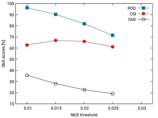
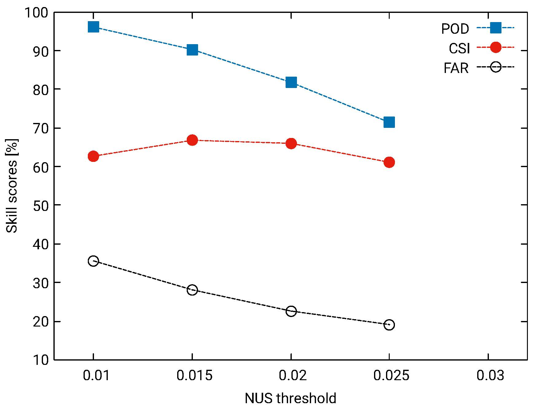
Figure 1. Simplified illustration of the generation of Cbs. Stage 1, towering cumulus; Stage 2, strong convection and updraft of the cloud (developing thunderstorm) leading to the generation of a mature Cb (Stage 3). Once the Cb has reached the tropopause, the updraft is retarded, and kinetic updraft energy is transmitted into vertical movement/development. This leads to the development of an anvil and subsequent dissipation of the Cb after a certain lifetime.
Remotesensing 11 00443 g001
Figure 2. SEVIRI normalized weighting function of MSG for clear sky, copyright (2002) EUMETSAT.
Remotesensing 11 00443 g002
Figure 3. Cloud regime dominated by stratiform clouds (advection). (Left) the BT of WV7.3 for 8 June 2017, 8:45 UTC. (Right) Normalized Updraft Strength (NUS) values for the same region, derived from the 8:45 and 9:00 UTC BT images. The NUS values are not significantly above zero, and no convection is indicated. For the complete region and time duration, lightning did not occur.
Remotesensing 11 00443 g003
Figure 4. Example of convective clouds and developing thunderstorms, 1 June 2017. (Top) the BT of the two water vapor channels (left: WV7.3, right: WV6.2) at 08:45 UTC. (Bottom left) The NUS values derived from the water vapor images (08:45 and 09:00). (Bottom right) Number of lightning events in a 0.05 × 0.05 degree resolution occurring +4–19 min after the satellite scan of the 09:00 image.
Remotesensing 11 00443 g004
Figure 5. Skill scores (POD, FAR, CSI) in % plotted against the NUS threshold for the 2016 (left) and 2017 (right) period and an SR of 32 km, respectively. Left: POD and FAR decreased with increasing NUS. CSI was relatively stable, but had the highest values around 0.015 for 2016 and 0.02 for 2017. For these experiments, the NWP filtering and the lightning settings were set in accordance with Experiment 1 in Table 1.
Remotesensing 11 00443 g005
Figure 6. Example of the effect of false alarms due to a frontal system in a low Convective Available Potential Energy (CAPE) environment (6 June 2017, 06 UTC). (Top) The image of the water vapor channel. The frontal system is apparent in the WV channel as a transition region with very dry (cloud-free) and very moist (cloudy) air. (Bottom) Image of the validation results. The red points are correctly-detected developing thunderstorms, while the black points with yellow background, indicating that CAPE is less than 60, are examples of false alarms in a low CAPE environment. In grey are false alarms that were successfully filtered out. In yellow are all regions where the NWP filtering (CAPE > 60 J/kg) would allow the detection of developing thunderstorms. Depending on the temperature gradients and CAPE, the frontal system could lead to the development of Cbs or false alarms.
Remotesensing 11 00443 g006
Figure 7. Illustration of the blurring effect on the observed NUS values. The objects colored in red stand for developing thunderstorms; the objects colored in grey stand for harmless clouds or missed detection caused by blurring. The values of the cell with an NUS value of 0.04 (left top) would be observed in the relevant satellite pixels as 0.01 (left bottom) because of its location, which is due to chance; whereas the cell with 0.022 and 0.014 (right top) would be observed close to their real values (right bottom). Assuming a threshold of 0.15, the largest cell would not be seen and counted as a missed detection. However, reducing the threshold of 0.1 would lead to an additional false alarm induced by the cell region with NUS of 0.12, and still, the large cell would be counted as a missed detection. Furthermore, the small cell with large updraft (right top) would not be apparent in the satellite observations. Thus, increasing the NUS threshold decreases FAR, but decreases POD, as well, and vice versa.
Remotesensing 11 00443 g007
Table 1. Results of the different experiments. NUS is as defined in Equation (3). Numerical Weather Prediction (NWP)/period provides the model used for NWP filtering (CAPE > 60 or TT > 50) and whether the investigated summer period was in 2016 or 2017. IFS is the forecast model of ECMWF. The other columns provide the probability of detection (POD), false alarm ratio (FAR) and the critical success index (CSI).
No.CI IfNWP/PeriodPOD (%)FAR (%)CSI (%)Time Lightning
1NUS > 0.02IFS/201681.822.666.0+4–19 min
2NUS > 0.02none/201685.928.663.8+4–19 min
3NUS > 0.015IFS/201690.328.166.8+4–19 min
4NUS > 0.015IFS/201688.625.168.3+4–29 min
5NUS > 0.02IFS/2017 I89.236.459.1+4–19 min
6NUS > 0.02none/201790.147.649.8+4–19 min
7NUS > 0.02IFS/2017 I87.632.561.6+4–29 min

