Automatic Land-Cover Mapping using Landsat Time-Series Data based on Google Earth Engine

Abstract

The Google Earth Engine (GEE) has emerged as an essential cloud-based platform for land-cover classification as it provides massive amounts of multi-source satellite data and high-performance computation service. This paper proposed an automatic land-cover classification method using time-series Landsat data on the GEE cloud-based platform. The Moderate Resolution Imaging Spectroradiometer (MODIS) land-cover products (MCD12Q1.006) with the International Geosphere–Biosphere Program (IGBP) classification scheme were used to provide accurate training samples using the rules of pixel filtering and spectral filtering, which resulted in an overall accuracy (OA) of 99.2%. Two types of spectral–temporal features (percentile composited features and median composited monthly features) generated from all available Landsat Thematic Mapper (TM) and Enhanced Thematic Mapper Plus (ETM+) data from the year 2010 ± 1 were used as input features to a Random Forest (RF) classifier for land-cover classification. The results showed that the monthly features outperformed the percentile features, giving an average OA of 80% against 77%. In addition, the monthly features composited using the median outperformed those composited using the maximum Normalized Difference Vegetation Index (NDVI) with an average OA of 80% against 78%. Therefore, the proposed method is able to generate accurate land-cover mapping automatically based on the GEE cloud-based platform, which is promising for regional and global land-cover mapping.

1. Introduction

Land-cover mapping and monitoring is one of the main applications of Earth observation satellite data [1], and is essential for the development and management of natural resource [2], modelling of environmental variables [3] and understanding of habitat distribution [4]. Due to the availability of a long-term data record going back to 1972 and the spatial resolution which can capture fine-grained land-cover patterns [5], images from the Landsat satellite series are an important data source for studying land-cover types and changes [6].

Recently, 30 m global land-cover products have been generated using training data which were interpreted visually from Landsat TM imagery together with a supervised classification method [7,8]. However, the manual selection of training data is labor-intensive and time-consuming, especially when mapping a large area. Therefore, much effort has focused on using training samples extracted from existing land cover maps to generate a Landsat-based land-cover product. For example, the National Agricultural Statistics Service (NASS) Cropland Data Layer (CDL) dataset [9] was incorporated into the training pool of the 2011 National Land Cover Database (NLCD) product [10]; the global Web-enabled Landsat Data (GWELD) were classified automatically using the training data derived from the Moderate Resolution Imaging Spectroradiometer (MODIS) land-cover product [11]; and The European Space Agency (ESA) Climate Change Initiative Global Land Cover (CCI_LC) product, combined with the MODIS Nadir Bidirectional Reflectance Distribution Function-Adjusted Reflectance (NBAR) product (MCD43A4), was used to extract the spatial–temporal spectral signature of each land-cover type in order to classify Landsat Operational Land Imager (OLI) imagery [12]. These studies have demonstrated that the use of existing land-cover maps as a source of training data can automatically generate accurate Landsat-based 30 m land-cover maps at the national and continental scale.

Due to the large volume of Landsat data involved, large data storage capacity, high computing power, and the ability to distribute algorithms were required to derive the 30 m land cover maps over large areas. Such requirements were available easily and free for everyone since the Google Earth Engine (GEE) has emerged. GEE is a cloud-based platform which consists of multi-source massive amounts of satellite data and high-performance computation service, making satellite imagery computing a relatively fast and flexible process [13]. Landsat-based classification in the cloud-based platform has been a widely used way of land cover mapping [14,15,16,17,18,19]. However, automatic land cover classification using satellite imagery and training samples extracted from existing land cover products based on GEE cloud-based platform were rarely investigated.

The availability of Landsat observations is affected by cloud cover and also by a sensor failure issue. Currently, two multi-temporal Landsat classification methods are widely used to eliminate the effects of missing observations caused by cloud cover or sensor failure. One is extracting metrics (such as the minimum, maximum, percentiles, etc.) of time-series of Landsat annual reflectance/vegetation index observations at the 30 m pixel level and classifying the metrics [11,20,21,22,23]. Another is making time-series of cloud-free composites of the Landsat images and then classifying the composites [24,25,26,27]. The two compositing methods are physically different. In the case of the metric composites, the pixel values of the same feature image have different acquisition times during the year and information on how the reflectance observations change with time is missing between metric features. For time-series of cloud-free composites, the change in reflectance with time is retained between temporal composites. However, comparative analysis of the classification performance and the effect of feature combinations on classification accuracy for these two methods have not been fully exploited.

The objective of this study was to develop a method for automatic 30 m land cover classification using MODIS land-cover products and Landsat data based on the GEE cloud-based platform. Multi-source and multi-temporal satellite imagery can be easily processed using this platform without the need to pay too much attention to the basic work of mosaicking, registration, projection conversion and resampling. The advantages of this platform make it convenient and flexible for use in land-cover classification, especially when a large number of features are used as input data. A novel method of sample collection using the MODIS land-cover product (MCD12Q1.006) based on a previous approach [11] was used. The proposed method resolved the issue of insufficient sample size and sample confusion for local-area mapping and was applied to three test areas in northern China. The automatically extracted samples were validated against historical high-resolution imagery in Google Earth. The Landsat TM/ETM+ surface reflectance products were consistently pre-processed using nadir Bidirectional Reflectance Distribution Function (BRDF) correction and illumination correction. Two type of spectral–temporal features (percentile composited features and median composited monthly features) were extracted from all available pre-processed TM/ETM+ data from the year 2010 ± 1 and used as input features to the RF classifier for land-cover classification in the three test areas. We investigated the difference in classification performance between percentile features and monthly features. In addition, we compared monthly features composited by median with that composited by maximum Normalized Difference Vegetation Index (NDVI), in terms of their land-cover characterization. Finally, the effect of feature combination and training-sample size on the classification accuracy were discussed for both the percentile features and the monthly features.

2. Study Area and Data

2.1. Study Area

The study area (Figure 1), which encompasses the Landsat footprint WRS-2 path/row 123/032, 125/034 and 125/033, was located in the north of China. The reasons for choosing these three scenes were (i) the Landsat TM/ETM+ imagery acquired in these areas has little cloud cover and so was expected to contain enough clear pixels to composite the cloud-free monthly imagery and accurate percentile imagery that we used in this study and (ii) the land-cover types in these areas are diverse, making it possible to test the effectiveness and robustness of the proposed method for areas with various land-cover types.

2.2. Landsat TM/ETM+ Data

The Landsat-5 and 7 satellites have the same sun-synchronous orbits and pass over the same location on the Earth’s surface every 16 days. Therefore, images acquired by the two different satellites are offset from each other by 8 days [28]. The Landsat-5 TM and Landsat-7 ETM+ sensors have a 15° field of view and 30 m spatial resolution, and their data are available as approximately 185 km × 180 km scenes which are defined in a Worldwide Reference System (WRS) of path and row coordinates [29]. The two sensors have similar reflectance bands and all TM/ETM+ band pairs also have similar spectral response functions [30]. Therefore, composites of Landsat TM and ETM+ images have been widely used to increase the temporal frequency of Landsat observations. All Landsat TM/ETM+ surface reflectance data from the year 2010 ± 1 available in GEE (a total of 92 images from path 123 and row 32, 89 images from path 125 and row 34 and 94 images from path 125 and row 33) were used in this study.

2.3. MODIS Land Cover Product

The MODIS Land Cover Type Product (MCD12Q1.006), which can be accessed in GEE, provides global land-cover maps at yearly intervals and 500 m spatial resolution from 2001 to present. As one of the layers in Collection 6 MCD12Q1 [31], the layers from the International Geosphere–Biosphere Program (IGBP) classification scheme are used to provide training class labels for Landsat-based land-cover classification. The IGBP classification scheme classifies each 500 m pixel into one of 17 classes—10 out of these 17 classes were used in this study. The class names, abbreviations and descriptions are summarized in

Table 1. Class names, abbreviations and descriptions of the 10 IGBP classes [32] used in this study.

Name	Abbreviation	Description
Evergreen needleleaf forest	ENF	Dominated by evergreen conifer trees (canopy >2 m). Tree cover >60%
Deciduous broadleaf forest	DBF	Dominated by deciduous broadleaf trees (canopy >2 m). Tree cover >60%
Mixed forest	MF	Dominated by neither deciduous nor evergreen (40–60% of each) tree type (canopy > 2 m). Tree cover >60%
Closed shrublands	CSL	Dominated by woody perennials (1–2 m height) >60% cover
Woody savannas	WS	Tree cover 30–60% (canopy > 2 m)
Savannas	SVN	Tree cover 10–30% (canopy > 2 m)
Grasslands	GRL	Dominated by herbaceous annuals (<2 m)
Croplands	CRL	At least 60% of area is cultivated cropland
Urban and built-up	UB	At least 30% impervious surface area including building materials, asphalt, and vehicles
Water	WTR	At least 60% of area is covered by permanent water bodies

. In addition, the IGBP “cropland/natural vegetation mosaic” class was discarded because we assumed that the mosaic of cropland and natural vegetation at a scale of 500 m scale can be separated at a scale of 30 m.

2.4. MODIS Nadir BRDF-Adjusted Reflectance Product

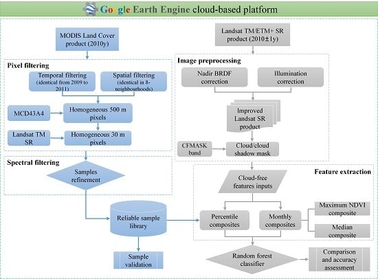
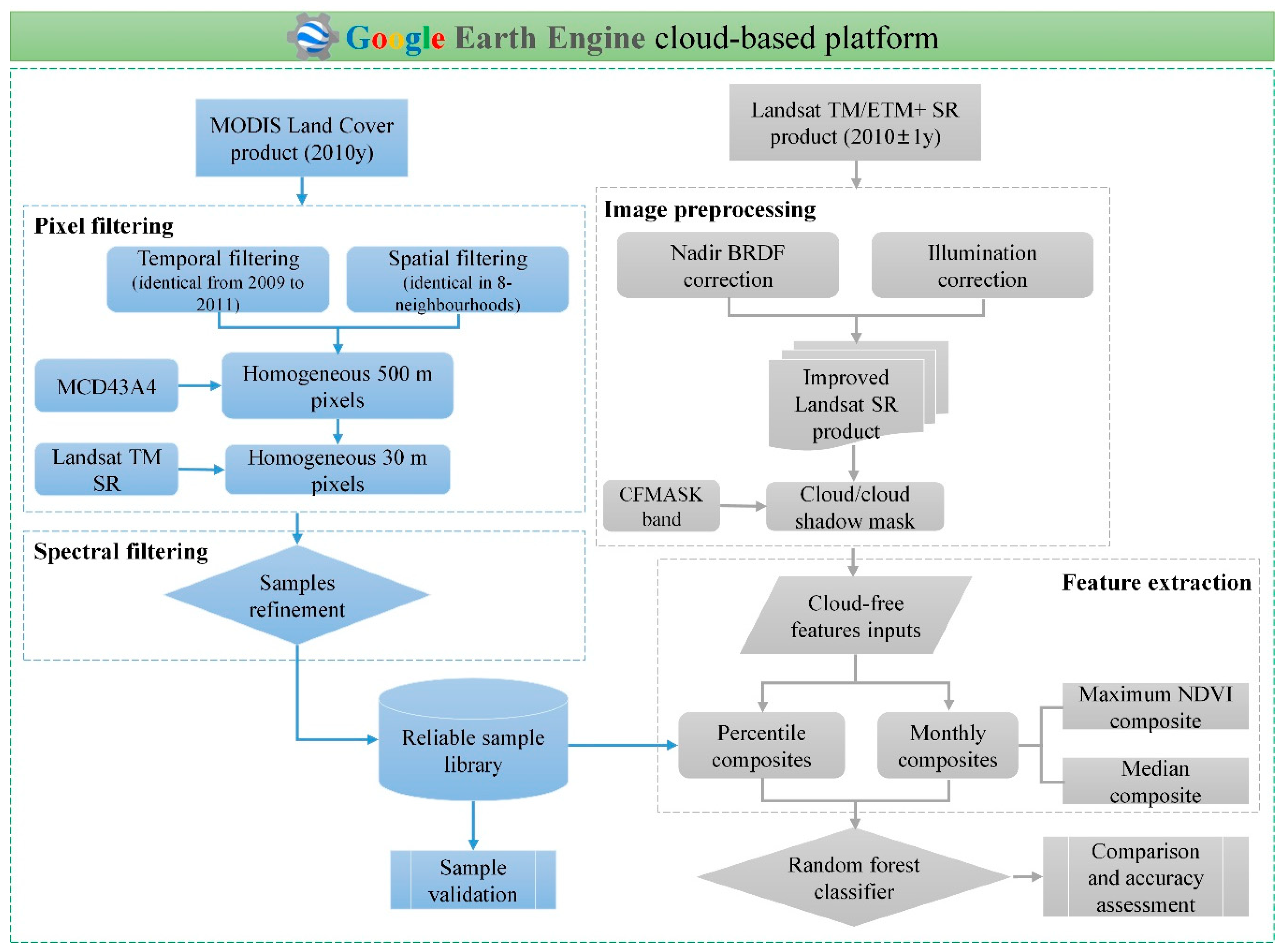
The nadir BRDF-adjusted reflectance (NBAR) product (MCD43A4) [33], which can also be accessed in GEE, provides daily 500 meter reflectance data for MODIS bands 1 through 7. These are adjusted using the BRDF model to remove the view-angle effects from the directional reflectances, resulting in a stable and consistent NBAR product. Bands 1–4, 6 and 7 of this product are used to determine the homogeneous 500 m pixels during the process of pixel filtering for MODIS land-cover products.

3. Method

The method (Figure 2) used in this study consisted of three parts. Firstly, the samples for each scene were extracted automatically using the MODIS land-cover products (MCD12Q1.006). A novel method of sample collection based on a previous approach [11] was used. Secondly, two typical feature-extraction methods were used for land-cover characterization. One involved extracting the percentiles from the annual Landsat reflectance time-series; the other method consisted of making monthly cloud-free images using median composites. In addition, the median composited monthly features were compared with the maximum NDVI composited monthly features, which are widely used in land-cover classification. Finally, based on the extracted samples and Landsat features, the land-cover types were classified using the random forest algorithm. All of these steps were performed on the GEE cloud-based platform.

GEE cloud-based platform provides massive amounts of multi-source satellite data and high-performance computation service, making the computation between different satellite imagery a relatively fast and flexible process. The MODIS and Landsat images can be easily resampled to the same spatial resolution (e.g., 30 meters) and transformed to the same map projection, e.g., Geographic Lat/Lon (EPSG:4326) using JavaScript codes on GEE cloud computing platform. Therefore, multi-source and multi-temporal satellite imagery can be easily processed using this platform without the need to pay too much attention to the basic work of mosaicking, registration, projection conversion and resampling.

3.1. Automatic Collection of Samples from MODIS Land Cover Products

MCD12Q1 products were used to select accurate training samples automatically; the selected samples were then used to extract Landsat spectral–temporal features which were used to train the classifier. This process aimed to automatically generate land-cover mapping at 30 m using Landsat data. The preliminary filtering criteria for MCD12Q1 products that were used are described below. These criteria were designed to help select only high-quality training class labels in which confidence was high:

(i)

the MCD12Q1 pixel values from 2009 to 2011 were identical;

(ii)

the MCD12Q1 pixels that had the same values in the 8 surrounding pixels for 2010;

(iii)

the 500 m MODIS pixels were homogeneous;

(iv)

the 30 m Landsat pixels within the 500 m MODIS pixel were homogenous.

Rule (i) selected the MCD12Q1 pixels that were consistently classified as belonging to the same land-cover class from 2009 to 2011. Rule (ii) helped to reduce 500 m pixel edge effects in situations where there were possible changes in the underlying land cover. Rule (iii) was introduced because the homogeneous pixels had a higher classification accuracy [34]. Rule (iv) helped to reduce the spectral variation within the 30 m pixels caused by heterogeneous pixels. The thresholds in

Table 2. Thresholds of value ranges used to determine homogeneous regions at the resolution of Landsat and MODIS imagery [35].

MODIS band	Landsat Band	Threshold
3	1	0.03
4	2	0.03
1	3	0.03
2	4	0.06
6	5	0.03
7	7	0.03

were used to identify homogeneous regions in the MODIS and Landsat imagery: within the 3 × 3 window, if the range of values was less than a predefined threshold then it was considered to be a homogeneous pixel.

In the previous approach [11], only one 30 m Landsat pixel within a filtered 500 m MODIS pixel was selected in order to reduce the data volume for mapping land cover at a continental scale. However, for the area covered by a Landsat scene (185 km × 180 km), a few 500 m MODIS pixels of land-cover type occupying a small area were left after preliminary filtering based on rules i, ii and iii. Therefore, using only one Landsat pixel per MODIS pixel may not be enough for the classifier to classify the land cover of local areas accurately. Due to the difference in spatial resolution, there are 17 × 17 (i.e., 289) Landsat pixels within one MODIS pixel. Consequently, all homogeneous Landsat pixels corresponding to the filtered MODIS pixel were selected and further steps were then taken to reduce the spectral variability of the 30 m pixels within the 500 m pixels. The details of this refinement (Rule v) are described below.

(a)

Calculate the spectral centroid of the sample set:

$${\rho }_c=median(\{{\rho }_i|i=1,2,\dots ,n\}),$$

(1)

$${\rho }_i=\left[{\rho }_i^{TM/ETM+1},{\rho }_i^{TM/ETM+2},{\rho }_i^{TM/ETM+3},{\rho }_i^{TM/ETM+4},{\rho }_i^{TM/ETM+5},{\rho }_i^{TM/ETM+7}\right],$$

(2)

where ${\rho }_i$ is a vector which consists of the reflectance values of the Landsat TM/ETM+ bands 1–5 and band 7; ${\rho }_c$ is the spectral centroid (a vector consisting of six Landsat TM/ETM+ surface reflectance values) and is the median value of a sample set in the spectral dimension.

(b)

Calculate the Euclidean distance from an individual sample to the spectral centroid of the sample set:

$${\Delta }_i=\sqrt{{{\displaystyle \sum }}_{j=1}^6{\left({\rho }_i^j–{\rho }_c^j\right)}^2},$$

(3)

where ${\Delta }_i$ is the Euclidean distance from sample i to the spectral centroid of the sample set.

(c)

Sort the calculated Euclidean distance from small to large and retain the top 50% of the samples.

A minority of heterogeneous 30 m pixels, which may have had land-cover types that were inconsistent with the 500 m MCD12Q1 pixels, were removed by the above refinement process. For samples with the same land-cover type, the spectral variability caused by the issue of mixed pixels was reduced and the spectral purity was improved significantly.

Therefore, the quality controls for MCD12Q1 pixels are Rule i, Rule ii and Rule iii; the quality controls for Landsat pixels within MCD12Q1 pixel are Rule iv and Rule v. That is to say, the MCD12Q1 pixels filtered by Rule i, ii and iii were used as polygons for Landsat data extraction. Therefore, not all those Landsat pixels belong to the correct class, only the Landsat pixels meet the requirement of Rule iv and Rule v are further considered to be the potential correct class.

3.2. Landsat TM/ETM+ Data Pre-Processing

The Landsat TM/ETM+ Surface Reflectance data in GEE were atmospherically corrected using the Landsat Ecosystem Disturbance Adaptive Processing System (LEDAPS), using a radiative transfer code with the aerosol characterization derived independently for each Landsat scene and external water vapor and ozone characterizations [36]. Using these data and the cloud-based platform, nadir BRDF correction was performed using a c-factor BRDF normalization method together with a fixed set of MODIS BRDF spectral model parameters [37] to normalize the forward and backward scattering difference in the area of overlap between the Landsat TM and ETM+ images. Topographic illumination correction was also carried using an empirical rotation model [38] to compensate for the solar irradiance, thus minimizing the variation in the reflectance of similar targets due to topography. For example, vegetation in the shadow of mountains may be confused with water in land-cover classification results. Compared with the cosine and C models, this model performs consistently well for both top-of-atmosphere and top-of-canopy Landsat reflectance data [39].

3.3. Landsat TM/ETM+ Composites

Due to the low temporal frequency, many of the images acquired by Landsat sensors are covered by cloud, which heavily limits actual data availability. In addition, the Landsat-7 ETM+ scan line corrector failed in May 2003, causing a 22% loss in data in each Landsat ETM+ image [40]. To improve data availability, pixel-based compositing of Landsat data has increased in popularity since the opening of the USGS Landsat archive in 2008 [41]. In this study, two types of spectral features—annual percentile composites [11,14,21] and monthly cloud-free composites [21,42]—were selected to characterize the land cover. Because cloud cover significantly limits the availability of Landsat images, all Landsat TM/ETM+ data from the year 2010 ± 1 that were available in the GEE were used to derive the metrics and monthly composites, irrespective of the acquisition year, in order to ensure that more cloud-free observations were available.

Based on the Landsat surface reflectance that was corrected using the GEE (Section 3.2), the 10th, 20th, 25th, 50th, 75th, 80th and 90th percentiles of annual time series observations of the TM/ETM+ reflectance bands and NDVI [43] were generated for use as the first type of spectral input; monthly cloud-free composites of the TM/ETM+ reflectance bands and NDVI from April to October were generated for use as the second type of spectral inputs. The composites for other months were discarded because of persistent cloud and snow [44]. Median composite technology was used to reduce each monthly group of images into a single composite on a per-pixel, per-band basis. The two types of Landsat-based compositing algorithms can be implemented easily and quickly on the GEE cloud-based platform. Before the compositing process was performed, areas of cloud, cloud shadow and snow in each Landsat image were masked using the CFMASK band of the Landsat SR product. Therefore, the percentile metric is extracted based on Landsat time-series “clear” (not contaminated by cloud, cloud shadow and snow) observations within the year; and monthly feature was derived based on Landsat multiple “clear” observations within the month.

In addition to the reflectance bands and NDVI, the 30 m digital elevation model (DEM), slope, and aspect bands derived from the Shuttle Radar Topography Mission (SRTM) data [45], were added to the feature inputs used for land-cover classification. The DEM, slope, and aspect features were involved because these variables were capacity of explaining the apparent variance caused by terrain factors within each class. Therefore, both compositing methods had a total of 52 band features; these are listed in

Table 3. Features inputs used for the land-cover characterization.

Type I Feature Inputs	Type II Features Inputs
10th percentile (TM/ETM+ band1-5, 7, NDVI)	Apr. (TM/ETM+ band1-5, 7, NDVI)
20th percentile (TM/ETM+ band1-5, 7, NDVI)	May (TM/ETM+ band1-5, 7, NDVI)
25th percentile (TM/ETM+ band1-5, 7, NDVI)	Jun. (TM/ETM+ band1-5, 7, NDVI)
50th percentile (TM/ETM+ band1-5, 7, NDVI)	Jul. (TM/ETM+ band1-5, 7, NDVI)
75th percentile (TM/ETM+ band1-5, 7, NDVI)	Aug. (TM/ETM+ band1-5, 7, NDVI)
80th percentile (TM/ETM+ band1-5, 7, NDVI)	Sep. (TM/ETM+ band1-5, 7, NDVI)
90th percentile (TM/ETM+ band1-5, 7, NDVI)	Oct. (TM/ETM+ band1-5, 7, NDVI)
DEM	DEM
Slope	Slope
Aspect	Aspect

.

3.4. Land-Cover Classification

The samples automatically selected from MCD12Q1.006 (Section 3.1) were used as training samples for land cover classification. The per-band pixel values of the stacked composited images were extracted from training samples and the resulting data were used to train Random Forest (RF) classifiers, which is the internal algorithm used in the GEE. The RF classifier is an ensemble machine learning algorithm which uses a set of CART decision trees to make predictions [46]. Each tree is created by randomly selected training samples and randomly selected features. New, unlabeled data is classified by all decision trees and the class with the maximum votes is the one that is finally selected. Two parameters need to be set to produce the forest trees: in this study, the number of decision trees (Ntree) was set to 100 and the user-defined number of features (Mtry) was kept at the default value (the square root of the number of input variables). The RF algorithm was chosen in this study given its superior ability to process features with a large number of dimensions, robustness to outliers and noise, and the higher classification accuracy obtained using the ensemble technique [47]. A land-cover map was generated for each test area using both compositing methods and the classification accuracy of each map was computed using the corresponding validation data sets.

3.5. Accuracy Assessment

The accuracy assessments of classification results were performed using a new independent stratified validation samples which were visually interpreted from very high resolution time series images of Google Earth. We have also used the System for Terrestrial Ecosystem Parameterization (STEP) sites which were drawn on Google Earth and used by the MCD12Q1 product, as well as the field photos from the Global Field Photo Library (eomf.ou.edu) for reference and understanding the spatial pattern of each land cover type. A total of 1375 samples from scene_123032, 1489 samples from scene_125034 and 1451 samples from scene_125033 were selected.

The traditional metrics, including user accuracy (UA), producer accuracy (PA) and overall accuracy (OA), were used to quantitatively evaluate the accuracy of classification. Kappa coefficient, a commonly used measure, was not used in this study, because it is highly correlated with overall accuracy [48]. Additionally, all the accuracy measures are adjusted with the area of each stratum (class) and presented with a 95% confidence interval [48].

4. Results and Discussion

4.1. Samples Automatically Extracted from MCD12Q1.006

The MCD12Q1.006 Land Cover (MLC) product was used to select samples for classifying the land cover in each selected Landsat scene. The MLC pixels which covered the same area as the corresponding Landsat scene were preliminarily filtered using rules (i), (ii), (iii) and (iv). The cloud-free images used for the selection of homogeneous MODIS and Landsat pixels for each scene are listed in

Table 4. Acquisition dates of cloud-free images used to select homogeneous 500 m and 30 m pixels.

Satellite	Scene_123032	Scene_125034	Scene_125033
MODIS (NBAR: MCD43A4.006)	20 May 2010	31 May 2009	31 May 2009
Landsat (Landsat-5 TM SR)	20 May 2010	31 May 2009	31 May 2009

. Figure 3 illustrates the process of preliminary filtration for MCD12Q1.006 from 2010 (Figure 3a), the 500 m pixels with consistent and reliable land cover types (Figure 3b), and the selected homogeneous 30 m pixels within each of the filtered 500 m pixels (Figure 3c).

Because the spatial resolution of MODIS is coarser than that of Landsat, the Landsat pixels within a given MODIS pixel may have outliers with different land-cover types. Generally, samples corresponding to the same land-cover type have similar spectral characteristics and form a band in a band–reflectance plot. The noisy samples have abnormal spectral curve shapes which should be removed to further refine the purity of the samples. Figure 4 illustrates the spectral features of a set of deciduous broadleaf forest samples before and after these were further refined using Rule v. It can be seen that, compared with beforehand, the homogeneity of the samples was improved significantly. In particular, the “Urban and built-up” samples with an annual maximum NDVI greater than 0.25 (experimentally obtained) were removed before further refinement based on Rule v because for small villages surrounded by cropland, the boundaries were indistinct at a scale of 500 m and the “Urban and built-up” samples were mixed with the “Croplands” type across the boundaries at the 30 m scale.

The sampling strategy used was stratified random sampling; i.e., random sampling was performed independently for each land-cover type according to the proportion of the MCD12Q1 area covered by the type. A total of 2749 samples from scene_123032, 3183 samples from scene_125034 and 2903 samples from scene_125033 were extracted. The number of training and validation samples for each land-cover type is shown in

Table 5. The number of training and testing samples, and the classification accuracy assessment for scene_123032. Accuracy measures are adjusted with the area of each class and presented with a 95% confidence interval.

Class	Tra.	Val.	Per.		Max.		Med.
			UA	PA	UA	PA	UA	PA
DBF	391	209	0.82 ± 0.05	0.84 ± 0.04	0.81 ± 0.05	0.83 ± 0.04	0.84 ± 0.05	0.89 ± 0.04
CSL	333	167	0.64 ± 0.07	0.56 ± 0.07	0.68 ± 0.07	0.55 ± 0.07	0.73 ± 0.07	0.59 ± 0.07
WS	274	126	0.80 ± 0.07	0.85 ± 0.06	0.76 ± 0.07	0.84 ± 0.06	0.85 ± 0.06	0.92 ± 0.04
SVN	326	174	0.66 ± 0.07	0.55 ± 0.06	0.73 ± 0.07	0.56 ± 0.06	0.82 ± 0.06	0.62 ± 0.06
GRL	529	271	0.72 ± 0.05	0.85 ± 0.04	0.75 ± 0.05	0.90 ± 0.03	0.76 ± 0.05	0.88 ± 0.04
CRL	468	232	0.79 ± 0.05	0.83 ± 0.04	0.81 ± 0.05	0.83 ± 0.03	0.81 ± 0.05	0.85 ± 0.03
UB	225	99	0.73 ± 0.10	0.55 ± 0.08	0.66 ± 0.10	0.56 ± 0.08	0.68 ± 0.10	0.57 ± 0.08
WTR	203	97	1.00 ± 0.00	1.00 ± 0.00	1.00 ± 0.00	1.00 ± 0.00	1.00 ± 0.00	1.00 ± 0.00
Total	2749	1375	0.75 ± 0.03		0.77 ± 0.03		0.79 ± 0.03

Note: “Tra.” represents the number of training samples for each class; “Val.” represents the number of validation samples for each class; “Per.” represents the classification result obtained using percentile features; “Max” represents the classification result obtained using maximum NDVI composited monthly features; and “Med.” represents the classification result obtained using median composited monthly features. The same for Table 6 and Table 7.

,

Table 6. The number of training and testing samples, and the classification accuracy assessment for scene_125034. Accuracy measures are adjusted with the area of each class and presented with a 95% confidence interval.

Class	Tra.	Val.	Per.		Max.		Med.
			UA	PA	UA	PA	UA	PA
ENF	85	42	0.97 ± 0.05	0.54 ± 0.20	1.00 ± 0.00	0.59 ± 0.18	0.97 ± 0.05	0.47 ± 0.24
DBF	254	130	0.95 ± 0.04	0.94 ± 0.04	0.99 ± 0.02	0.94 ± 0.04	0.98 ± 0.03	0.96 ± 0.03
MF	396	189	0.91 ± 0.04	0.79 ± 0.06	0.89 ± 0.05	0.82 ± 0.06	0.91 ± 0.04	0.83 ± 0.05
CSL	264	126	0.93 ± 0.04	0.87 ± 0.11	0.97 ± 0.03	0.86 ± 0.09	0.94 ± 0.04	0.82 ± 0.13
WS	342	138	0.80 ± 0.07	0.82 ± 0.08	0.82 ± 0.06	0.82 ± 0.08	0.85 ± 0.06	0.91 ± 0.05
SVN	474	211	0.76 ± 0.06	0.72 ± 0.09	0.77 ± 0.05	0.74 ± 0.09	0.82 ± 0.05	0.82 ± 0.08
GRL	543	237	0.66 ± 0.05	0.98 ± 0.01	0.66 ± 0.05	0.98 ± 0.01	0.68 ± 0.05	0.98 ± 0.01
CRL	512	288	0.92 ± 0.04	0.68 ± 0.04	0.89 ± 0.04	0.71 ± 0.04	0.89 ± 0.04	0.70 ± 0.04
UB	173	72	0.78 ± 0.11	0.51 ± 0.10	0.84 ± 0.10	0.44 ± 0.09	0.79 ± 0.11	0.47 ± 0.09
WTR	140	56	1.00 ± 0.00	1.00 ± 0.00	1.00 ± 0.00	1.00 ± 0.00	1.00 ± 0.00	1.00 ± 0.00
Total	3183	1489	0.78 ± 0.03		0.79 ± 0.03		0.80 ± 0.03

and

Table 7. The number of training and testing samples, and the classification accuracy assessment for scene_125033. Accuracy measures are adjusted with the area of each class and presented with a 95% confidence interval.

Class	Tra.	Val.	Per.		Max.		Med.
			UA	PA	UA	PA	UA	PA
DBF	325	175	0.91 ± 0.04	0.92 ± 0.05	0.95 ± 0.03	0.88 ± 0.07	0.95 ± 0.03	0.94 ± 0.04
MF	239	116	0.93 ± 0.05	0.88 ± 0.08	0.92 ± 0.05	0.88 ± 0.09	0.93 ± 0.05	0.91 ± 0.09
CSL	351	149	0.80 ± 0.06	0.74 ± 0.09	0.79 ± 0.06	0.69 ± 0.09	0.86 ± 0.05	0.82 ± 0.11
WS	56	43	0.97 ± 0.06	0.17 ± 0.09	0.97 ± 0.05	0.35 ± 0.21	0.97 ± 0.05	0.50 ± 0.22
SVN	416	184	0.77 ± 0.06	0.67 ± 0.08	0.76 ± 0.06	0.78 ± 0.07	0.84 ± 0.05	0.80 ± 0.07
GRL	511	289	0.73 ± 0.05	0.97 ± 0.01	0.76 ± 0.04	0.97 ± 0.01	0.75 ± 0.04	0.97 ± 0.01
CRL	452	248	0.82 ± 0.05	0.71 ± 0.05	0.82 ± 0.05	0.74 ± 0.05	0.84 ± 0.05	0.73 ± 0.05
UB	334	166	0.98 ± 0.03	0.28 ± 0.05	0.91 ± 0.05	0.35 ± 0.06	0.92 ± 0.05	0.34 ± 0.06
WTR	219	81	1.00 ± 0.00	1.00 ± 0.00	1.00 ± 0.00	1.00 ± 0.00	1.00 ± 0.00	1.00 ± 0.00
Total	2903	1451	0.77 ± 0.03		0.79 ± 0.03		0.80 ± 0.03

for each scene.

4.2. Validation of the Automatically Extracted Samples

To investigate the reliability of the samples extracted by the proposed method, the extracted samples were validated using an image interpretation method based on the historical high-resolution imagery in Google Earth, which is widely used to select samples used for land-cover classification. We randomly selected one thousand samples (one hundred for each land-cover types) from the automatically generated sample database to validate the accuracy of the samples. The error rate and accuracy for each sample type and the whole set of samples are shown in Figure 5. The confusion matrix is shown in Table S1. The sample accuracy for grasslands, croplands, and urban and built-up were 98%, 99% and 95%, respectively. The sample accuracy for the remaining land-cover types was 100%. The overall accuracy of all the samples was 99.2%. These validation results demonstrate that the samples extracted by the proposed method were reliable for use in land-cover classification because the RF classifier used in this study was insensitive to noise as long as the noise threshold of 20% was not exceeded [1].

4.3. The Landsat-based Classification Results

Using the samples automatically selected by the proposed method, classification of land cover using the Landsat imagery was performed. The classification results for each scene obtained using percentile features and median composited monthly features are shown in Figure 6b,d, respectively. From a visual comparison, the spatial patterns of the land-cover types are similar for the two sets of results. The number of training and validation samples, the classification accuracy assessment (including UA, PA and OA) for each scene are given in Table 5, Table 6 and Table 7. Accuracy measures are adjusted by the area of each stratum (class) and presented with a 95% confidence interval. All the confusion matrixes are shown in Tables S2–S10. As can be clearly seen, the OA of the classification results based on median composited monthly features are 79%, 80% and 80% for scene_123032, scene_125034 and scene_125033, respectively; and those based on the percentile features are 75%, 78% and 77% for scene_123032, scene_125034 and scene_125033, respectively. The average OA of the former (80%) is higher than that of the latter (77%). In the case of the single-type results, for most land-cover types, the producer accuracy was higher for the results obtained using the median composited monthly features than for the results obtained using the percentile features. A comparison of the results thus demonstrates that, in terms of multitemporal Landsat classification, the performance of the monthly composited features was superior to that of the percentile composited features. The time-series monthly features retain phenological information about the land cover and so perform better at land-cover characterization. The percentile features were affected by the number of valid observations: even though as many Landsat data as possible were used to derive the percentile features, the number of valid observations still varied from pixel to pixel.

In addition, the median composite method was compared to the maximum NDVI composite method, which is a method commonly applied to monthly cloud-free composited images [21]. The particular observation—not cloud-contaminated or missing—corresponding to the maximum NDVI in the specific temporal range (i.e., one month) was used for compositing. The classification results obtained using the maximum NDVI composited monthly features for each scene are shown in Figure 6c. As shown in Table 5, Table 6 and Table 7, the OA of the classification results that were based on the maximum NDVI composited monthly features were 77%, 79% and 79% for scene_123032, scene_125034 and scene_125033, respectively. The average OA of this compositing method (78%) was lower than that based on the median composited monthly features (80%). A comparison of these results thus also shows that the median composite method was superior to the maximum NDVI composite method for constructing cloud-free time-series of spectral features. Therefore, it can be concluded that land-cover types can be more accurately characterized by monthly median composited features.

As can be seen in Table 5, Table 6 and Table 7, the accuracies of the same land cover type were not identical in different regions. Based on the classification results obtained by median composited monthly features, CSL, WS, SVN and UB have greater difference in producer accuracy (more than 20%) between different regions while DBF, GRL, CRL and WTR have smaller difference in producer accuracy (less than 15%). Region-specific climate and environmental condition usually lead to the variation of spatial pattern and spectral features of the same land cover type. This also highlighted the importance of independent classification of geographic strata.

Based on the results obtained by median composited monthly features, the average producer accuracy was used to compare the differences between single class accuracies. The single classes, sorted by PA in descending order are WTR, GRL, DBF, WS, CRL, SVN, CSL and UB. Therefore, water, grasslands and deciduous broadleaf forest classes have the top three highest producer accuracy while closed shrublands and urban classes have the two lowest accuracies. For classification results obtained by monthly features, the average OA with the median method is slightly higher than that with the maximum NDVI method. However, GRL have higher producer accuracy with the maximum NDVI method, while DBF, CSL, WS, SVN and UB have better producer accuracy with the median method. CRL and WTR have the same accuracy with either maximum NDVI or median method. Furthermore, no significantly better result was obtained with the two methods combined.

In addition, the differences of class area between MODIS classification and the resulting classification of this study were compared and analyzed. The area statistics of land cover class for MODIS land cover product and the resulting Landsat-based classification were illustrated in Figure 7. As can be clearly seen, except for grassland and cropland, most land cover types have no significant area difference among the four classification results. In scene_123032 and scene_125033, the area of grassland type derived from MODIS classification is substantially larger than that derived from Landsat-based results. Additionally, the area of cropland type derived from MODIS classification is obviously smaller in scene_123032 and scene_125033, and slightly larger in scene_125034. The comparison results demonstrated that the scale effect of satellite imagery has great influence on the area of grassland and cropland cover type.

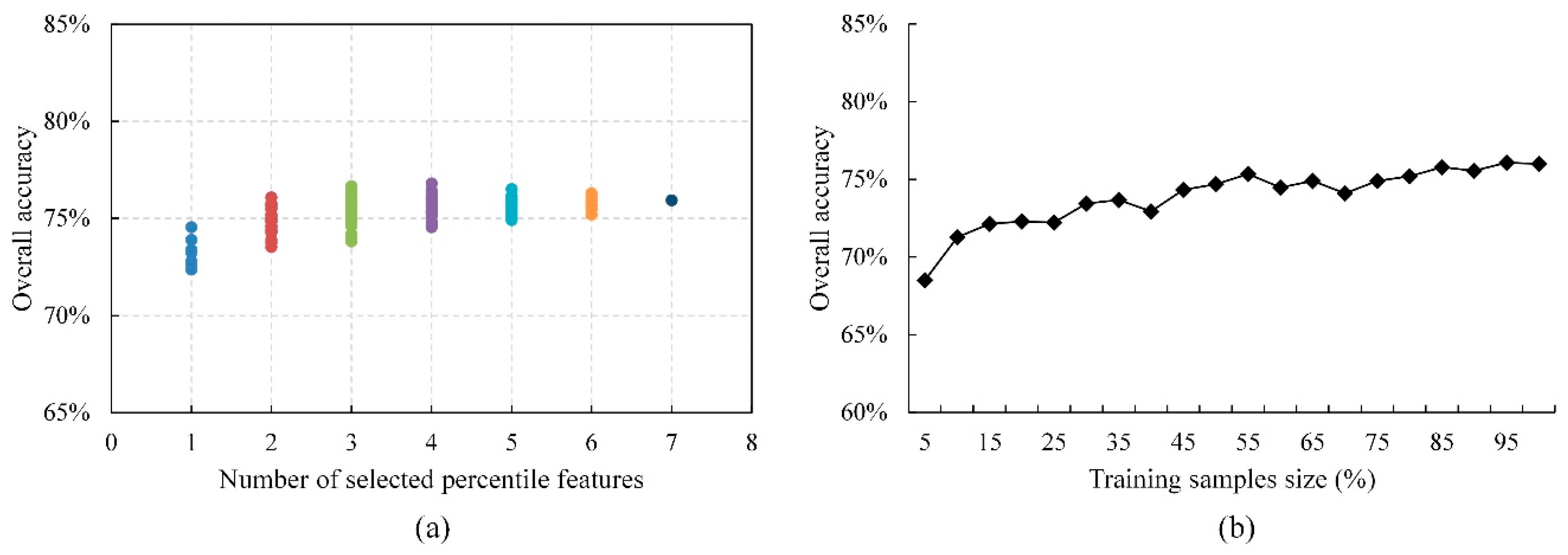
4.4. Effect of Feature Combinations and Training-Sample Size

Multitemporal satellite images are widely used in land-cover classification [49]. Because using single-date imagery to identity land-cover types with similar spectral features can be challenging [50,51], multitemporal images have been employed to make use of the phenological variation which is a valuable information source for improving the accuracy of land-cover classification [52]. However, in terms of land-cover classification, the usefulness of information does not always increase in proportion to the number of multitemporal images [53]. For example, the separability between land cover types was found to be highest using images from December and January, and lowest using images from July and August [54]; the classification accuracy achieved by using Landsat images from all four seasons was higher than that achieved by using single-season imagery for land-cover classification in urban areas [55].

In this section, the effect of feature combination on classification accuracy is fully explored for the two types of feature input based on the RF classifier. Features were randomly combined based on the mathematical principles of permutation and combination (i.e., $C_n^m$ equals the number of combinations when m features are taken from n features). The OA measurement, which was derived based on validation samples, was used to quantitatively evaluate the performance for each feature combination. Figure 8a and Figure 9a illustrate the classification accuracy of each feature combination for the specific number of selected percentile/monthly features (from 1 to 7). The results demonstrate that different combinations of the same number of features produced different classification accuracies and that the range of variation for the percentile features was smaller than that for the monthly features. However, RF gave a higher overall accuracy with an increased number of percentile or monthly features, which was more evident in the case of the monthly features than for the percentile features.

In addition, the effect of the training-sample size on the classification accuracy was assessed for the two types of feature input based on the RF classifier and for the validation samples. The effect of the training-sample size was evaluated using the OA by altering the size of the training sets in increments of 5%, from 5% to 95%. Figure 8b and Figure 9b illustrate the relationship between the size of the training sample and classification accuracy. It can be seen that both the percentile and monthly features had a low sensitivity to the training-sample size. For an increase in sample size from 5% to 95%, the overall accuracy changed from 68% to 76% (an 8% increase) for the percentile features and from 67% to 80% (an 13% increase) for the monthly features. Thus, for the percentile features, the accuracy changed by less as the number of training data increased than it did in the case of the monthly features. However, the relative increase in OA as the training-sample size increased was similar for both percentile and monthly features.

5. Conclusions

The intention of this study was to develop a method for automatic land-cover mapping at a scale of 30 m based on the Google Earth Engine cloud-based platform. A novel method for automatic collection of training samples was proposed based on previous approaches to resolve the issues of insufficient sample size and sample confusion in local-area mapping. MCD12Q1.006 land-cover products were used to provide reliable training class labels based on the rules of pixel filtering and spectral filtering. All available Landsat TM/ETM+ data acquired in the study area from the year 2010 ± 1 were used for the land-cover classification. Two types of spectral-temporal features (percentile composited features and median composited monthly features) were used for characterizing the land cover. In addition, the monthly features composited using the median were compared with those composited using the maximum NDVI, the latter being a commonly used method for temporal compositing of images. The following conclusions can be drawn.

(i)

The samples automatically extracted by the proposed method were reliable and accurate with an overall accuracy of 99.2%;

(ii)

Both the percentile features and monthly features produced excellent land- cover classification results; however, the classification produced using the median composited monthly features was more accurate than that obtained using the percentile features – average overall accuracy of 80% against 77%. In addition, the monthly features composited using the median values outperformed those composited using the maximum NDVI values in terms of the classification performance – average overall accuracy of 80% against 78%;

(iii)

For single class accuracy, WTR, GRL and DBF have the top three highest producer accuracy while CSL and UB have the two lowest accuracies, based on median composited monthly features. Additionally, GRL have higher producer accuracy with the maximum NDVI method, while DBF, CSL, WS, SVN and UB have better producer accuracy with the median method;

(iv)

Higher overall accuracies were achieved with an increased number of percentile or monthly features. Both the percentile and monthly features had a low sensitivity to the training-sample size and the OA increased as the size of the training samples increased.

Therefore, the method proposed in this paper was able to achieve land-cover classification for Landsat data automatically, quickly and accurately based on the Google Earth Engine cloud-based platform. These results are of great significance to regional and global land-cover mapping.

References

1. Rodriguez-Galiano, V.F.; Ghimire, B.; Rogan, J.; Chica-Olmo, M.; Rigol-Sanchez, J.P. An assessment of the effectiveness of a random forest classifier for land-cover classification. ISPRS J. Photogramm. Remote Sens. 2012, 67, 93–104. [Google Scholar] [CrossRef]
2. Gómez, C.; White, J.C.; Wulder, M.A. Optical remotely sensed time series data for land cover classification: A review. ISPRS J. Photogramm. Remote Sens. 2016, 116, 55–72. [Google Scholar] [CrossRef] [Green Version]
3. Herold, M.; Latham, J.; Di Gregorio, A.; Schmullius, C. Evolving standards in land cover characterization. J. Land Use Sci. 2006, 1, 157–168. [Google Scholar] [CrossRef] [Green Version]
4. Sesnie, S.E.; Gessler, P.E.; Finegan, B.; Thessler, S. Integrating landsat tm and srtm-dem derived variables with decision trees for habitat classification and change detection in complex neotropical environments. Remote Sens. Environ. 2008, 112, 2145–2159. [Google Scholar] [CrossRef]
5. Pflugmacher, D.; Cohen, W.B.; Kennedy, R.E. Using landsat-derived disturbance history (1972–2010) to predict current forest structure. Remote Sens. Environ. 2012, 122, 146–165. [Google Scholar] [CrossRef]
6. Zhu, Z.; Woodcock, C.E. Continuous change detection and classification of land cover using all available landsat data. Remote Sens. Environ. 2014, 144, 152–171. [Google Scholar] [CrossRef] [Green Version]
7. Chen, J.; Chen, J.; Liao, A.; Cao, X.; Chen, L.; Chen, X.; He, C.; Han, G.; Peng, S.; Lu, M. Global land cover mapping at 30 m resolution: A pok-based operational approach. ISPRS J. Photogramm. Remote Sens. 2015, 103, 7–27. [Google Scholar] [CrossRef] [Green Version]
8. Gong, P.; Wang, J.; Yu, L.; Zhao, Y.; Zhao, Y.; Liang, L.; Niu, Z.; Huang, X.; Fu, H.; Liu, S. Finer resolution observation and monitoring of global land cover: First mapping results with landsat tm and etm+ data. Int. J. Remote Sens. 2013, 34, 2607–2654. [Google Scholar] [CrossRef] [Green Version]
9. Johnson, D.M.; Mueller, R. The 2009 cropland data layer. PERS Photogramm. Eng. Remote Sens. 2010, 76, 1201–1205. [Google Scholar]
10. Homer, C.; Dewitz, J.; Yang, L.; Jin, S.; Danielson, P.; Xian, G.; Coulston, J.; Herold, N.; Wickham, J.; Megown, K. Completion of the 2011 national land cover database for the conterminous united states–representing a decade of land cover change information. Photogramm. Eng. Remote Sens. 2015, 81, 345–354. [Google Scholar]
11. Zhang, H.K.; Roy, D.P. Using the 500 m modis land cover product to derive a consistent continental scale 30 m landsat land cover classification. Remote Sens. Environ. 2017, 197, 15–34. [Google Scholar] [CrossRef]
12. Zhang, X.; Liu, L.; Chen, X.; Xie, S.; Gao, Y. Fine land-cover mapping in china using landsat datacube and an operational speclib-based approach. Remote Sens. 2019, 11, 1056. [Google Scholar] [CrossRef] [Green Version]
13. Gorelick, N.; Hancher, M.; Dixon, M.; Ilyushchenko, S.; Thau, D.; Moore, R. Google earth engine: Planetary-scale geospatial analysis for everyone. Remote Sens. Environ. 2017, 202, 18–27. [Google Scholar] [CrossRef]
14. Azzari, G.; Lobell, D. Landsat-based classification in the cloud: An opportunity for a paradigm shift in land cover monitoring. Remote Sens. Environ. 2017, 202, 64–74. [Google Scholar] [CrossRef]
15. Chen, B.; Xiao, X.; Li, X.; Pan, L.; Doughty, R.; Ma, J.; Dong, J.; Qin, Y.; Zhao, B.; Wu, Z. A mangrove forest map of china in 2015: Analysis of time series landsat 7/8 and sentinel-1a imagery in google earth engine cloud computing platform. ISPRS J. Photogramm. Remote Sens. 2017, 131, 104–120. [Google Scholar] [CrossRef]
16. Dong, J.; Xiao, X.; Menarguez, M.A.; Zhang, G.; Qin, Y.; Thau, D.; Biradar, C.; Moore III, B. Mapping paddy rice planting area in northeastern asia with landsat 8 images, phenology-based algorithm and google earth engine. Remote Sens. Environ. 2016, 185, 142–154. [Google Scholar] [CrossRef] [Green Version]
17. Goldblatt, R.; Stuhlmacher, M.F.; Tellman, B.; Clinton, N.; Hanson, G.; Georgescu, M.; Wang, C.; Serrano-Candela, F.; Khandelwal, A.K.; Cheng, W.-H. Using landsat and nighttime lights for supervised pixel-based image classification of urban land cover. Remote Sens. Environ. 2018, 205, 253–275. [Google Scholar] [CrossRef]
18. Huang, H.; Chen, Y.; Clinton, N.; Wang, J.; Wang, X.; Liu, C.; Gong, P.; Yang, J.; Bai, Y.; Zheng, Y. Mapping major land cover dynamics in beijing using all landsat images in google earth engine. Remote Sens. Environ. 2017, 202, 166–176. [Google Scholar] [CrossRef]
19. Patel, N.N.; Angiuli, E.; Gamba, P.; Gaughan, A.; Lisini, G.; Stevens, F.R.; Tatem, A.J.; Trianni, G. Multitemporal settlement and population mapping from landsat using google earth engine. Int. J. Appl. Earth Obs. Geoinf. 2015, 35, 199–208. [Google Scholar] [CrossRef] [Green Version]
20. Beckschäfer, P. Obtaining rubber plantation age information from very dense landsat tm & etm+ time series data and pixel-based image compositing. Remote Sens. Environ. 2017, 196, 89–100. [Google Scholar]
21. Hansen, M.C.; Egorov, A.; Roy, D.P.; Potapov, P.; Ju, J.; Turubanova, S.; Kommareddy, I.; Loveland, T.R. Continuous fields of land cover for the conterminous united states using landsat data: First results from the web-enabled landsat data (weld) project. Remote Sens. Lett. 2011, 2, 279–288. [Google Scholar] [CrossRef]
22. Mack, B.; Leinenkugel, P.; Kuenzer, C.; Dech, S. A semi-automated approach for the generation of a new land use and land cover product for germany based on landsat time-series and lucas in-situ data. Remote Sens. Lett. 2017, 8, 244–253. [Google Scholar] [CrossRef]
23. Potapov, P.V.; Turubanova, S.; Tyukavina, A.; Krylov, A.; McCarty, J.; Radeloff, V.; Hansen, M. Eastern europe’s forest cover dynamics from 1985 to 2012 quantified from the full landsat archive. Remote Sens. Environ. 2015, 159, 28–43. [Google Scholar] [CrossRef]
24. Griffiths, P.; van der Linden, S.; Kuemmerle, T.; Hostert, P. A pixel-based landsat compositing algorithm for large area land cover mapping. IEEE J. Sel. Top. Appl. Earth Obs. Remote Sens. 2013, 6, 2088–2101. [Google Scholar] [CrossRef]
25. Hansen, M.C.; Roy, D.P.; Lindquist, E.; Adusei, B.; Justice, C.O.; Altstatt, A. A method for integrating modis and landsat data for systematic monitoring of forest cover and change in the congo basin. Remote Sens. Environ. 2008, 112, 2495–2513. [Google Scholar] [CrossRef]
26. Hermosilla, T.; Wulder, M.A.; White, J.C.; Coops, N.C.; Hobart, G.W. Regional detection, characterization, and attribution of annual forest change from 1984 to 2012 using landsat-derived time-series metrics. Remote Sens. Environ. 2015, 170, 121–132. [Google Scholar] [CrossRef]
27. Hermosilla, T.; Wulder, M.A.; White, J.C.; Coops, N.C.; Hobart, G.W. Disturbance-informed annual land cover classification maps of Canada’s forested ecosystems for a 29-year landsat time series. Can. J. Remote Sens. 2018, 44, 67–87. [Google Scholar] [CrossRef]
28. Teillet, P.; Barker, J.; Markham, B.; Irish, R.; Fedosejevs, G.; Storey, J. Radiometric cross-calibration of the landsat-7 etm+ and landsat-5 tm sensors based on tandem data sets. Remote Sens. Environ. 2001, 78, 39–54. [Google Scholar] [CrossRef] [Green Version]
29. Arvidson, T.; Goward, S.; Gasch, J.; Williams, D. Landsat-7 long-term acquisition plan. Photogramm. Eng. Remote Sens. 2006, 72, 1137–1146. [Google Scholar] [CrossRef]
30. Claverie, M.; Vermote, E.F.; Franch, B.; Masek, J.G. Evaluation of the landsat-5 tm and landsat-7 etm+ surface reflectance products. Remote Sens. Environ. 2015, 169, 390–403. [Google Scholar] [CrossRef]
31. Sulla-Menashe, D.; Gray, J.M.; Abercrombie, S.P.; Friedl, M.A. Hierarchical mapping of annual global land cover 2001 to present: The modis collection 6 land cover product. Remote Sens. Environ. 2019, 222, 183–194. [Google Scholar] [CrossRef]
32. Sulla-Menashe, D.; Friedl, M.A. User Guide to Collection 6 Modis Land Cover (mcd12q1 and mcd12c1) Product; USGS: Reston, VA, USA, 2018.
33. Schaaf, C.; Wang, Z. Mcd43a4 Modis/Terra+ Aqua brdf/Albedo Nadir brdf Adjusted Refdaily l3 global-500 m v006; NASA EOSDIS Land Processes DAAC: Washington, DC, USA, 2015.
34. Wang, Z.; Liu, L. Assessment of coarse-resolution land cover products using casi hyperspectral data in an arid zone in northwestern china. Remote Sens. 2014, 6, 2864–2883. [Google Scholar] [CrossRef] [Green Version]
35. Feng, M.; Huang, C.; Channan, S.; Vermote, E.F.; Masek, J.G.; Townshend, J.R. Quality assessment of landsat surface reflectance products using modis data. Comput. Geosci. 2012, 38, 9–22. [Google Scholar] [CrossRef] [Green Version]
36. Masek, J.G.; Vermote, E.F.; Saleous, N.E.; Wolfe, R.; Hall, F.G.; Huemmrich, K.F.; Gao, F.; Kutler, J.; Lim, T.-K. A landsat surface reflectance dataset for north america, 1990–2000. IEEE Geosci. Remote Sens. Lett. 2006, 3, 68–72. [Google Scholar] [CrossRef]
37. Roy, D.P.; Zhang, H.; Ju, J.; Gomez-Dans, J.L.; Lewis, P.E.; Schaaf, C.; Sun, Q.; Li, J.; Huang, H.; Kovalskyy, V. A general method to normalize landsat reflectance data to nadir brdf adjusted reflectance. Remote Sens. Environ. 2016, 176, 255–271. [Google Scholar] [CrossRef] [Green Version]
38. Tan, B.; Masek, J.G.; Wolfe, R.; Gao, F.; Huang, C.; Vermote, E.F.; Sexton, J.O.; Ederer, G. Improved forest change detection with terrain illumination corrected landsat images. Remote Sens. Environ. 2013, 136, 469–483. [Google Scholar] [CrossRef]
39. Tan, B.; Wolfe, R.; Masek, J.; Gao, F.; Vermote, E.F. In An Illumination Correction Algorithm on Landsat-tm Data. In Proceedings of the IEEE International Geoscience and Remote Sensing Symposium, IEEE, Honolulu, HI, USA, 25–30 July 2010; pp. 1964–1967. [Google Scholar]
40. Markham, B.L.; Storey, J.C.; Williams, D.L.; Irons, J.R. Landsat sensor performance: History and current status. IEEE Trans. Geosci. Remote Sens. 2004, 42, 2691–2694. [Google Scholar] [CrossRef]
41. Woodcock, C.E.; Allen, R.; Anderson, M.; Belward, A.; Bindschadler, R.; Cohen, W.; Gao, F.; Goward, S.N.; Helder, D.; Helmer, E. Free access to landsat imagery. Science 2008, 320, 1011. [Google Scholar] [CrossRef]
42. Roy, D.P.; Ju, J.; Kline, K.; Scaramuzza, P.L.; Kovalskyy, V.; Hansen, M.; Loveland, T.R.; Vermote, E.; Zhang, C. Web-enabled landsat data (weld): Landsat etm+ composited mosaics of the conterminous united states. Remote Sens. Environ. 2010, 114, 35–49. [Google Scholar] [CrossRef]
43. Richardson, A.J.; Wiegand, C.L. Distinguishing vegetation from soil background information. Photogramm. Eng. Remote Sens. 1977, 43, 1541–1552. [Google Scholar]
44. Ju, J.; Roy, D.P. The availability of cloud-free landsat etm+ data over the conterminous united states and globally. Remote Sens. Environ. 2008, 112, 1196–1211. [Google Scholar] [CrossRef]
45. Farr, T.G.; Rosen, P.A.; Caro, E.; Crippen, R.; Duren, R.; Hensley, S.; Kobrick, M.; Paller, M.; Rodriguez, E.; Roth, L. The shuttle radar topography mission. Rev. Geophys. 2007, 45. [Google Scholar] [CrossRef] [Green Version]
46. Breiman, L. Random forests. Mach. Learn. 2001, 45, 5–32. [Google Scholar] [CrossRef] [Green Version]
47. Belgiu, M.; Drăguţ, L. Random forest in remote sensing: A review of applications and future directions. ISPRS J. Photogramm. Remote Sens. 2016, 114, 24–31. [Google Scholar] [CrossRef]
48. Olofsson, P.; Foody, G.M.; Herold, M.; Stehman, S.V.; Woodcock, C.E.; Wulder, M.A. Good practices for estimating area and assessing accuracy of land change. Remote Sens. Environ. 2014, 148, 42–57. [Google Scholar] [CrossRef]
49. Cihlar, J. Land cover mapping of large areas from satellites: Status and research priorities. Int. J. Remote Sens. 2000, 21, 1093–1114. [Google Scholar] [CrossRef]
50. Liu, J.; Zhuang, D.; Luo, D.; Xiao, X.M. Land-cover classification of china: Integrated analysis of avhrr imagery and geophysical data. Int. J. Remote Sens. 2003, 24, 2485–2500. [Google Scholar] [CrossRef]
51. Vieira, C.; Mather, P.; Aplin, P. Multitemporal classification of agricultural crops using the spectral-temporal response surface. In Analysis of Multi-Temporal Remote Sensing Images; World Scientific: Singapore, 2002; pp. 290–297. [Google Scholar]
52. Knight, J.F.; Lunetta, R.S.; Ediriwickrema, J.; Khorram, S. Regional scale land cover characterization using modis-ndvi 250 m multi-temporal imagery: A phenology-based approach. GIScience Remote Sens. 2006, 43, 1–23. [Google Scholar] [CrossRef]
53. Carrão, H.; Gonçalves, P.; Caetano, M. Contribution of multispectral and multitemporal information from modis images to land cover classification. Remote Sens. Environ. 2008, 112, 986–997. [Google Scholar] [CrossRef]
54. Nitze, I.; Barrett, B.; Cawkwell, F. Temporal optimisation of image acquisition for land cover classification with random forest and modis time-series. Int. J. Appl. Earth Obs. Geoinf. 2015, 34, 136–146. [Google Scholar] [CrossRef] [Green Version]
55. Zhu, Z.; Woodcock, C.E.; Rogan, J.; Kellndorfer, J. Assessment of spectral, polarimetric, temporal, and spatial dimensions for urban and peri-urban land cover classification using landsat and sar data. Remote Sens. Environ. 2012, 117, 72–82. [Google Scholar] [CrossRef]
Figure 1. The location of the study areas which were shown in Landsat TM true color composites. The numeric labels correspond to path/row designations. Noted that the three path/rows were referred to as “scene_123032”, “scene_125033” and “scene_125034”, respectively, for the reminder of the article.
Remotesensing 11 03023 g001
Figure 2. Flowchart showing the main steps of the proposed method used in this study.
Remotesensing 11 03023 g002
Figure 3. Illustration of preliminary selection of colocated 500 m and 30 m pixels. (a) Sample MCD12Q1.006 500 m Land Cover Product (a sub-region of scene_125034, covering approximately 102 × 96 km) for the year 2010; (b) filtered 500 m MODIS pixels based on rules (i), (ii) and (iii); and (c) filtered 30 m Landsat pixels based on Rule (iv).
Remotesensing 11 03023 g003
Figure 4. Spectral features of examples of deciduous broadleaf forest samples before and after refinement.
Remotesensing 11 03023 g004
Figure 5. The error rate and accuracy for the samples automatically extracted by the proposed method (Abbreviations on the x-axis correspond to different land-cover classes: see Table 1).
Remotesensing 11 03023 g005
Figure 6. The three sets of classification results for the three test Landsat scenes: (a) the original Landsat imagery displayed as TM bands 4-3-2 for R-G-B; (b) the classification results based on percentile features; (c) the classification results based on maximum NDVI composited monthly features; and (d) the classification results based on median composited monthly features.
Remotesensing 11 03023 g006
Figure 7. The area statistics of land cover classes for MODIS land cover product and the resulting Landsat-based classification. (a) scene_123032; (b) scene_125034; (c) scene_125033.
Remotesensing 11 03023 g007
Figure 8. Effects of feature combination (a) and training-sample size increase (b) on the classification accuracy for percentile features.
Remotesensing 11 03023 g008
Figure 9. Effects of feature combination (a) and training-sample size increase (b) on the classification accuracy for monthly features.
Remotesensing 11 03023 g009