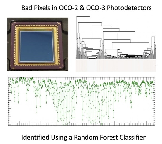
Classification of Anomalous Pixels in the Focal Plane Arrays of Orbiting Carbon Observatory-2 and -3 via Machine Learning

Abstract

A machine learning approach was developed to improve the bad pixel maps that mask damaged or unusable pixels in the imaging spectrometers of National Aeronautics and Space Administration (NASA) Orbiting Carbon Observatory-2 (OCO-2) and Orbiting Carbon Observatory-3 (OCO-3). The OCO-2 and OCO-3 instruments use nearly 500,000 pixels to record high resolution spectra in three infrared wavelength ranges. These spectra are analyzed to retrieve estimates of the column-average carbon dioxide (XCO${}_2$) concentration in Earth’s atmosphere. To meet mission requirements, these XCO${}_2$ estimates must have accuracies exceeding 0.25%, and small uncertainties in the bias or gain of even one detector pixel can add significant error to the retrieved XCO${}_2$ estimates. Thus, anomalous pixels are identified and removed from the data stream by applying a bad pixel map prior to further processing. To develop these maps, we first characterize each pixel’s behavior through a collection of interpretable and statistically well-defined metrics. These features and a prior map are then used as inputs in a Random Forest classifier to assign a likelihood that a given pixel is bad. Consequently, the likelihoods are analyzed and thresholds are chosen to produce a new bad pixel map. The machine learning approach adopted here has improved data quality by identifying hundreds of new bad pixels in each detector. Such an approach can be generalized to other instruments that require independent calibration of many individual elements.

1. Introduction

The identification of various undesirable artifacts in imaging spectrometer data plays an important role in the quality and accuracy of the subsequent products. The declined quality can impact the analysis and interpretation of the resulting images, for example, for target and event detection in astronomy [1], anomaly, and change detection in terrestrial or planetary geologic studies [2], or the evaluation of absorption features to retrieve the abundance of various atmospheric gases [3]. Such artifacts are usually persistent features of the detector that can be due to manufacturing defects; however, they can also develop during instrument operations. Bad pixels in the focal plane array (FPA) are the smallest individual elements of the detector exhibiting anomalous or degraded behavior. FPAs usually consist of hundreds of thousands or millions of pixels, so, even if a small fraction of the detector is inoperable, it can have a considerable impact on the resulting images or measured spectra. The large number of individual pixels also necessitates an algorithmic approach that can scale to the size and cannot rely on manual analysis of each pixel.

The issues associated with bad pixels are well-known and the main types of such pixels have been described [1,4,5]. For example, pixels can be considered bad if they record a high digital number (DN) or, on the other hand, do not respond to any amount of illumination. The most commonly used bad pixel detection method is thresholding of pixel summary statistics obtained from dark calibration or illuminated flat-field images. If some derived value for a pixel is greater than a certain threshold, such as a certain number of standard deviations away from a mean or a median, then it is declared bad. Examples of summary statistics include standard deviations [6], mean absolute second differences and signal-to-noise ratios [5], and coefficients of variation [7]. A considerable sample of methods rely on nearest neighbor comparisons and collect metrics that describe relationships in the spatial and/or spectral dimensions, which in turn are thresholded to obtain bad pixels [2,4,8,9]. Principal Component Analysis (PCA) on a set of detector images is also used for the identification of bad pixels that appear different from the “background" or good pixel space [10,11]. Finally, another proposed technique [1] uses a probabilistic approach. The authors first perform a Gaussian Mixture Model clustering of a pairwise pixel distance measure and then rank pixels according to the probabilities of the clusters with the highest distances that were obtained from multiple image datasets. Most of the cited work performs both detection and interpolation of bad pixel values at the same time, where most of the interpolations are based on median filters or nearest neighbors.

The imaging spectrometers carried by the NASA OCO-2 and OCO-3 missions record high resolution spectra of reflected sunlight in three spectral ranges, and these spectra are combined and analyzed with remote sensing retrieval algorithms to yield spatially resolved estimates of XCO${}_2$ with single sounding precisions near 0.125% and regional scale accuracies of ∼0.25% [12,13]. These high precision and accuracy requirements place unprecedented demands on the radiometric and spectroscopic calibration of these space-based sensors. Incorrect measurements from bad pixels can propagate through the retrieval system into a biased or noisy XCO${}_2$ measurement. Another challenge for bad pixel detection for these two instruments is that the FPAs used by OCO-2 are flight-spare units from the original OCO mission and were manufactured in 2006, while those for OCO-3 were manufactured using a new process but have been in warm storage for several years. As a result, there has been more degradation, especially for OCO-2, with certain parts of the FPA having either clusters or large amounts of random bad pixels such that even robust summary statistics, i.e., median, can be skewed. Neighbor comparisons could also break down due to a large proportion of neighbors being bad.

In addition, identifying bad pixels for OCO-2 and OCO-3 is challenging due to the large data volume (both number of pixels and mission duration) along with the diversity of the undesirable behaviors, e.g., instability or degradation due to radiation and thermal cycles. Moreover, since both instruments are in the harsh environment of space, the events triggering the anomalous behavior of pixels are much more common, and the bad pixel map that masks bad pixels in the flight software needs to be updated. Both instruments, however, collect calibration and various telemetry data daily, including dark and illuminated flat-field images of the FPAs. These routinely obtained images provide a rich data source for bad pixel detection.

We present a new approach to detect and identify anomalous pixels in the FPAs of OCO-2 and OCO-3 using a traditional machine learning algorithm [14,15]. We define the detection of bad pixels as a binary classification problem. Instead of examining and thresholding individual summary statistics or distance measures, we compute a set of features and use them collectively in a model that is trained to assign a likelihood to each pixel of being bad. The features are computed on a time series spanning the whole mission. The corresponding input for training the model is the previously developed bad pixel map. Finally, we seek to maintain interpretability of the results and provide insights into the model and pixel behavior. Thus, we develop a statistically rigorous approach that improves the accuracy of the existing mask and largely automates the development of any future mask. Our work does not focus on bad pixel interpolation or de-noising and filtering of the images since the algorithms to apply the bad pixel map are already implemented in flight software.

The remainder of the paper is organized in three sections. In Section 2, we briefly introduce OCO-2 and OCO-3 instruments, and describe the features and the classification model. Section 3 reports the results and the approach for selecting bad pixels based on the likelihoods obtained from classification. Section 4 offers a a discussion of future directions, and the final section provides the conclusions.

2. Data and Methods

The OCO-2 and OCO-3 spectrometers use nearly 500,000 pixels to measure three near-infrared bands with high resolution. The three channels measure the O${}_2$ ABO2 band at $0.765\mathsf{\mu }$m, the “weak” CO${}_2$ (WCO2) band at $1.61\mathsf{\mu }$m, and the “strong” CO${}_2$ (SCO2) band at $2.06\mathsf{\mu }$m. At the focus of each spectrometer is a Teledyne Hawaii-1RG (Teledyne Imaging Sensors, Camarillo, CA, USA) FPA consisting of 1024 × 1024 pixels that measure 18 $\mathsf{\mu }$m by 18 $\mathsf{\mu }$m each. The O${}_2$ detector is Si, while the CO${}_2$ detectors are HgCdTe. The OCO-2 detectors were procured as spares for the OCO mission, while the OCO-3 detectors used a newer process. The columns of the detector record different wavelengths, while rows record different field angles. Due to the narrow spectrometer slit, only 220 rows near the middle are read out. Of these, roughly 180 rows are illuminated, and the middle 160 of those rows form the science area and are used to retrieve CO${}_2$. While the field of view across the slit is spatially-resolved across 160 of its science rows, the spectrum is dispersed across 1024 of the FPA columns. To reduce data volume, the rows are averaged into eight spatial footprints; thus, an array of 8 × 1024 is returned for science. Because this summation is performed on board, prior to bias and gain corrections, individual pixels that are dead or respond anomalously to light or the instrument environment must be identified and eliminated from the sum. Figure 1 shows images of the three full FPAs in the dark. For more information on the FPA, related components and the OCO-2 and OCO-3 instruments themselves please refer to [16,17,18].

A bad pixel map is a binary array, where 0 indicates a good pixel and 1 indicates a bad pixel. This map is uploaded to the flight computer to prevent the data from these pixels being included in the downlinked “summed” science data, called “samples”. If one or two pixels are bad, they are replaced by the average of the two adjacent good pixels in the spatial dimension to obtain the final sum of the 20 pixels; however, if three or more continuous pixels are bad, those values are excluded from the sum and the weights of the remaining pixels are renormalized. This operation is performed by the flight software on-board the instruments and was implemented in an early stage of the original OCO mission. It is clear that, if a bad pixel remains in the sum downlinked to Earth, it can greatly contaminate the corresponding measurement. It is also important to note that, because the individual pixel data are not returned to the ground, the masking of bad pixels cannot be reversed or improved. There does exist a diagnostic “pixel mode” where all 220 rows are returned at a greatly reduced frame rate. This is essential for calibration but is not practical for science data collection. In this work, we use the calibration “pixel mode" data that contains the full array of pixel measurements before the summation is performed.

Bad pixel identification begins before launch during thermal-vacuum (TVAC) testing and continues in-flight. In TVAC, single pixel data are collected every few hours at the beginning of each procedure. During flight, the data are taken over a dozen times per day when the spacecraft is over the dark side of the Earth. In both cases, the instrument views the onboard calibrator in the dark and also obtains “flat-field” lamp images by illuminating a diffuser with a tungsten halogen lamp.

The collected dark and “flat-field” lamp images, both measuring 220 × 1024 pixels, in uncalibrated DN, are the two data sources used for bad pixel identification. These images are obtained from uncalibrated Level 1A instrument data products [17]. In this work, the DN values from these images are transformed into a collection of interpretable and statistically well-defined features that are then input into a machine learning model that is trained to differentiate between bad and good pixels. The computed features are summary statistics that capture a variety of pixel characteristics including similarity to neighbors, temporal trends, and instability.

2.1. Data Normalization

While dark images can be readily used to derive model features, the “flat-field” lamp images require normalization to allow comparison of pixels from different regions of the detector. The overall lamp intensity varies with time, but more importantly there are spectral and spatial gradients in the illumination that reaches the FPA. The first step is to subtract the dark signal from the lamp images using the dark image acquired closest in time, usually within a few minutes. This correction ensures that the lamp signal is not confounded with the dark signal. The dark-corrected lamp images are then normalized by iterative row-wise robust scaling, i.e., subtraction of median and division by the interquartile range, $\mathrm{IQR}=Q_3-Q_1$, where $Q_1$ and $Q_3$ are the 25th and 75th percentiles of a distribution of all pixel values in that row. Median and IQR are robust to large outliers, which is important when the dataset includes many bad pixels. An example of the normalized and dark-corrected “flat-field" lamp images is shown in Figure 2.

From a set of dark and normalized lamp images, we obtain time series data for each pixel i, $i=1,\dots ,N$, where N is the number of pixels, representing the time-varying DN dark or lamp signal, $z_i=(z_{i,1},\dots z_{i,T})$, with $t=1,\dots ,T$, and where T is the total number of images. These time series are contaminated by outlier frames, including several very large outliers due to cosmic ray hits. We assume that these are isolated, mostly random events that produce big spikes in the data; thus, we compute an outlier threshold for each pixel i based on the IQR of the pixel DN signal:

$$\begin{array}{c}\hfill c_i=Q_{3,i}+a·(Q_{3,i}-Q_{1,i}),\end{array}$$

where $Q_1$ and $Q_3$ are defined as the 25th and the 75th percentile of the time-varying distribution for a pixel i and a is a scaling constant. The outliers are removed if $|z_{i,t}|>c_i$, with dark and lamp time series screened individually. After these two pre-processing steps, normalization of lamp images and removal of signal outliers, the data are ready to be used for feature extraction.

2.2. Characterizing Pixel Behavior and Feature Extraction

Generally, good pixels are stable with time and similar to their neighbors. The mean signal and noise level of good pixels vary across the detector due to manufacturing and instrument properties. Examples of such properties are the “W-pattern” in the ABO2 band, shown as regularly-spaced vertical lines in Figure 1 and “hot” rows in the WCO2 and SCO2 bands, represented by white horizontal lines in Figure 1. Bad pixels’ responses, on the other hand, are diverse, which creates challenges in their identification. In order to capture bad pixel behavior, we compute several metrics and summary statistics that could describe the range of possible abnormal behavior. We use these collectively in a machine learning model, which makes it possible to capture interactions and nonlinear relationships.

All pixels, even good ones, exhibit some level of signal-independent background noise as well as a photon noise component that is roughly proportional to the square root of incident radiance. To mitigate the impact of noise on the features and in order to quantify the information about the variability in each signal, we pre-process the time series with a wavelet transform [15]. The raw signal is first deconstructed by fitting a set of orthonormal basis functions to the data, then the coefficients of the basis functions are either sub-selected or their magnitude is reduced [19]. The sparse or reduced coefficients are consequently applied to reconstruct a smoothed version of the raw signal. A variety of such basis function families exist; however, we use the Haar basis [20] for their simplicity and because they produce piecewise-constant signal representations. Since they are not continuous, they have the advantage of being able to capture abrupt transitions. Once a DN time series $z_i$ without outliers is constructed, we apply the Haar wavelet transform and keep 50% of the largest coefficients, corresponding to the coarsest decomposition levels, thus obtaining a smoothed reconstructed DN signal ${\tilde{z}}_i$. See an example of such a reconstructed signal in Figure 3 as a black line through the raw signal displayed in red.

The minimum and maximum of this reconstructed DN signal, $max\left({\tilde{z}}_i\right)$ and $min\left({\tilde{z}}_i\right)$, are used directly as features to capture pixels that are unresponsive to light or pixels that exhibit abnormally high dark current or sensitivity. Additional features that use the wavelet reconstructed signal are the standard deviation, which captures noise, and the jumping score to register sudden transitions:

$$x_i^{\mathrm{jump}}=\underset{t}{max}\left(\{\left|{\tilde{z}}_{i,t}-{\tilde{z}}_{i,t-1}\right|:t=2,\cdots T\}\right),$$

(1)

which is the maximum value of the absolute differences of the reconstructed signal. Bad pixels have larger transitions and/or transition more frequently, which is particularly problematic for both science measurements and in-flight calibration updates that combine several days of data. Over time, thermal cycles, power cycles, and exposure to cosmic rays may have introduced sudden changes for what were previously good pixels. An example of such discontinuities can be seen in Figure 3b and a corresponding differenced wavelet-smoothed signal is presented in Figure 3c.

Since the input illumination is continuous, a good pixel should not differ much from the adjacent good pixels. In addition, the good pixels in the special areas of the FPA, e.g., “W-pattern”, would be different from the rest, but similar to each other. Therefore, the final feature that is computed based on the DN time series is a comparison with its neighbors. We use Dynamic Time Warping (DTW) [21,22] to measure the dissimilarity between each pair of pixels. Given two time series $z_i$ and $z_{i^{\prime }}$, DTW first populates a matrix of pairwise distances between each point in $z_i$ and to each point in $z_{i^{\prime }}$. This matrix contains all possible “warp" paths $P=(p_1,\dots ,p_s,\dots ,p_k)$, where $p_s=(j_s,j_s^{\prime })$ is a pair of indices in $z_i$ and $z_{i^{\prime }}$ that connect the bottom left of the matrix to the top right. Each point $p_s$ of a “warp" path P has a corresponding distance between the two respective elements of the time series, $d(j_s,j_s^{\prime })$. Then, a “warp" path P with the minimum overall distance is found using dynamic programming. The overall distance for this optimal path is the final DTW distance measure between the two time series. For example, if the two time series $z_i$ and $z_{i^{\prime }}$ are identical, the optimal “warp" path P would be along the diagonal of the pairwise distance matrix, i.e., $P=((1,1),(2,2),\dots ,(T_i,T_{i^{\prime }}))$, where $T_i$ and $T_{i^{\prime }}$ are the sizes of $z_i$ and $z_{i^{\prime }}$, respectively; however, a “warp” path for non-identical time series would most probably contain pairs of indices that are located off the diagonal of the distance matrix. We chose an approximate but fast implementation of DTW [23] since the standard DTW algorithm has quadratic time and space complexity and is computationally expensive. The DTW metric is computed for the nearest neighbors of each pixel and the minimum of these values are taken as a feature:

$$\begin{array}{c}\hfill x_i^{\mathrm{dtw}}=\underset{i^{\prime }\in N_i}{min}\left(\mathrm{dtw}(z_i,z_{i^{\prime }})\right),\mathrm{dtw}(z_i,z_{i^{\prime }})=\frac{1}{T_i+T_{i^{\prime }}}\underset{P}{min}\left(\sum _{s=1}^{k}d(j_s,j_s^{\prime })\right),\end{array}$$

(2)

where $T_i$ and $T_{i^{\prime }}$ are again the sizes of $z_i$ and $z_{i^{\prime }}$, $N_i$ are the indices of the nearest neighbors of $z_i$ and $|N_i|=8$. The distance $d(·)$ is Euclidean. DTW is able to ignore when the time series are shifted or not aligned globally or locally since it does not compare each point in time t in one time series with the matched time t in another time series. The pixel time series are usually not well aligned due to the outlier removal. Moreover, good pixel signals can slightly vary around the same time step t due to measurement noise, as mentioned previously, which makes DTW more robust than simply computing a pairwise Euclidean distance. Examples of DTW for bad and a good pixels and how they can compress the information about a pixel’s nearest neighbors are shown in Figure 4.

Lamp and dark signal have been found to be coupled to various instrument temperatures, including those of the FPA, optical bench assembly (OBA), remote electronics module, and, for OCO-3, the telescope [24]. One set of features used is the Pearson correlation coefficient between DN and select temperatures for both dark and lamp data:

$$\begin{array}{c}\hfill x_i^{\mathrm{corr}}=\frac{{\sum }_t(z_{i,t}-{\overline{z}}_i)(h_{i,t}-{\overline{h}}_i)}{\sqrt{{\sum }_t{(z_{i,t}-{\overline{z}}_i)}^2}\sqrt{{\sum }_t{(h_{i,t}-{\overline{h}}_i)}^2}},\end{array}$$

(3)

where $h_i=(h_1,\dots ,h_T)$ is a vector of temperature values, obtained for each image t and ${\overline{h}}_i$ and ${\overline{z}}_i$ are means of $h_i$ and $z_i$, respectively.

We summarize the computed features in

Table 1. List of features used in the classifier.

Feature (Dark and Lamp)	Description
Minimum	responsiveness	$x_i^{\min }=min\left({\tilde{z}}_i\right)$
Maximum	sensitivity	$x_i^{\max }=max\left({\tilde{z}}_i\right)$
Jumping Score	change with time	$x_i^{\mathrm{jump}}$ (1)
Noise	instability	$x_i^{\mathrm{std}}=\mathrm{std}(z_i-{\tilde{z}}_i)$
Dynamic Time Warping	similarity to neighbors	$x_i^{\mathrm{dtw}}$ (2)
Temperature Correlations	FPA, OBA and other: 6 (OCO-2) and 4 (OCO-3)	$x_i^{\mathrm{corr}}$ (3)

. All of the features, except DTW and temperature correlations, use the wavelet-smoothed signal. DTW is more robust to noise in the time series, while temperature correlations use the raw time series $z_i$ to preserve the thermal sensitivity. The extracted features represent the majority of aberrant pixel behavior and can capture the main differences between good and bad pixels. Pixels could thus be differentiated not only by one feature, but by several jointly, which can vary for each individual pixel. Figure 5 shows examples of the computed dark residual standard deviation and lamp maximum DN values for OCO-2 SCO2 band, displayed as histograms that are separated by good and bad classes of pixels. Figure 5 shows that dark residual standard deviation is more effective in separating the bad pixels for this band; however, not all of them will be separated by this feature, as the existence of a small mode on the left shows. The bad pixels in this mode are captured by other features. Lamp DN maximum, on the other hand, does not explain most of the bad pixels in this band; however, it can identify various individual outliers.

2.3. Random Forest Classification

The features described in the section above are computed for each pixel and are combined into vectors, which in turn form a matrix of features of size $N\times p$, where p is the number of features, used as a direct input into a multivariate classification model. We selected Random Forest [14] for its simplicity, computational speed, superior performance in a great variety of settings, and the ability to capture nonlinear relationships without explicitly specifying the model. Random Forests are extremely well-known and hugely popular. They are based on randomized ensembles of decision trees that are averaged to greatly reduce the variability inherent in such models.

While the input variables into the Random Forest are the features extracted from each pixel’s time series $z_i$, the output variable for the model is a vector $y_i\in [0,1]$ of size N of binary responses indicating whether a pixel is good or bad. The labels $y_i$ are obtained from a previously developed bad pixel mask and serve as the “prior” information. The “a priori” mask was developed with the previous bad pixel identification methodology that analyzed dark signal magnitude and lamp noise individually. The “a priori” mask represents the best expert knowledge as to what pixels might be currently bad and will be used in training the machine learning to differentiate pixel behavior. With a machine learning classification model, we therefore seek to improve on this mask by identifying new bad pixels and re-labeling bad pixels that were previously marked good. While it would be possible to also change bad pixels to good, we choose not to do so for reasons explained in Section 3.

In classification where the output is a binary variable, one of the criteria for the performance of a trained model is a confusion matrix computed using the “true” input labels and the model predicted labels. This specifies the counts of false positives, i.e., good pixels that were erroneously identified as bad, false negatives, i.e., bad pixels that were classified as good, and true positive and true negatives, i.e., bad or good pixels correctly identified. Customarily, lower false positive and false negative rates are desirable and are used to tune and evaluate the model. However, for this particular problem the false positives, and to a lesser degree false negatives, are of interest since they represent the potential new bad (or good) pixels we aim to identify.

We perform training and testing with stratified 3-fold cross-validation, where about 67% of the pixels are used to train the model and about 33% are used to test the model, with equal proportions of bad and good pixels guaranteed in each test set. We iterate the cross-validation process 50 times. A likelihood that each pixel is bad is collected for each iteration and for each cross-validation fold based on the withheld test data. The likelihoods are then averaged across all iterations to obtain one final likelihood estimate.

3. Results and Discussion

The likelihoods produced by the classifier model compress the available information about pixel behavior and provide a simple unified metric for the detection of bad pixels. After the likelihoods are obtained from the classifier, a threshold needs to be determined to update the final bad pixel map. Traditionally, likelihood cutoffs for binary classification are based on either controlling the rate of false positives or false negatives, depending on the application. Then, for any prediction with the trained model on a new data point, the likelihood is first computed based on the model and the chosen threshold is applied to determine class membership. In this work, the thresholds are determined based on the distribution of the likelihoods and such that there is an acceptable number of false positives, i.e., new bad pixels. OCO-2 and OCO-3 had slightly different approaches since the former had been in flight for over three years and the latter was still undergoing TVAC testing.

3.1. Joint Distributions of Likelihood Statistics

In order to choose the bad pixel thresholds, we obtain likelihoods from several classification models, trained on different time periods. We then calculate summary statistics of these likelihoods for each pixel and combine these statistics as joint distributions, where each point in the distribution represents a pixel. The joint distributions of the likelihood summary statistics are visualized to determine approximate thresholds and further fine-tuned by adjusting the number of false positives. OCO-2 and the recently launched OCO-3 instruments undergo regular decontaminations, when heaters are used to drive out water ice that has accumulated with time. These decontamination events are potential triggers for some pixels to change behavior, so they are natural places to break the data record to train separate models.

For OCO-2, 11 decontamination cycles were used spanning the period from the beginning of the mission in September 2014 to August 2018. We then computed the minimum and standard deviation of the resulting 11 likelihoods for each pixel, and visualized the joint distributions of these statistics in Figure 6. The overwhelming majority of the pixels, roughly 98%, are good and have the corresponding likelihood statistics near $(0,0)$. The thresholds are chosen for both minimum and standard deviation of the likelihoods, and are placed such that most of the pixels in the long tails of the distribution are declared bad. The upper left quadrant of each plot in Figure 6 shows pixels with a minimum close to zero but with relatively high standard deviation, indicating that these pixels are unstable and may have been impacted by the decontamination cycles. In the bottom right quadrant, the pixels have been consistently bad throughout the mission. Most of such pixels, especially at the end of the long tail, where the minimum is 1 and standard deviation is about 0, have been marked as bad with previous methodology and are very clear cases of anomalous behavior. Then, in the upper right quadrant, the pixels exhibit both instability across decontamination cycles and relatively high likelihoods.

Fine-tuning the final thresholds is based on the desired number of false positives, where the expected number is based on instrument knowledge. Figure 6d–f demonstrate how the thresholds can be adjusted using cumulative distribution functions of false positives. In Figure 6b, for example, the approximate threshold for the WCO2 band could be somewhere between 15–30% for the likelihood minimum, corresponding to 99.9% of the distribution, but the number of false positives obtained closer to 15% would give a more reasonable and conservative estimate, or around 500 instead of 100 new bad pixels, as shown in Figure 6e. The threshold of 10% is too tight and would have doubled the number of new bad pixels to around 1000, with most of them representing “borderline” cases.

The resulting false positives are important since they represent potential new bad pixels, while the false negatives, on the other hand, are much less important for the creation of the bad pixel map. Once a pixel is declared bad, it will stay masked, and any false negatives will be ignored. The reason for this is that an erroneous inclusion of a bad pixel as good is disproportionately worse than declaring a good pixel bad. The impact of a false negative, replacing a good pixel with the average of its neighbors, is negligible because the good pixel and its neighbors are very similar.

For OCO-3, the bad pixel map was initially developed using one TVAC time period, with the thresholds determined by directly examining the univariate distribution of likelihoods. Once in-orbit, the bad pixel map was updated based on the data from a subsequent TVAC and also during two periods of the in-orbit checkout (IOC), the first one spanning the first week of the instrument taking data in space and the second IOC period spanning the third week. The thresholds were then determined by using the joint distribution of the likelihood maximum from the new TVAC and the first IOC and of the likelihoods obtained from the second IOC. The likelihood comparisons and the cutoff thresholds for the OCO-3 bad pixel map are shown in Figure 7. The joint distributions are similar to those for OCO-2, but the minimum and the standard deviations of the likelihoods are replaced by the second IOC likelihood value and the maximum of TVAC and first IOC, respectively. The lower right quadrant of the distributions in Figure 7 is sparse, indicating that most of the clear bad pixel cases were detected in the previous TVAC. The populated upper left quadrant, however, shows that some currently good or “borderline” pixels exhibited anomalous behavior previously, more specifically in the latest TVAC. The final thresholds were chosen such that the pixels that displayed anomalous behavior either in TVAC or on-orbit were declared bad.

3.2. Tree Interpreter

Another diagnostic tool we use is the tree interpreter [25]. The tree interpreter is a tool that determines which features contributed to the increase or decrease of the likelihood for each pixel. The tree interpreter considers the overall ratio of bad to good pixels as an a priori estimate of the likelihood. Then, it evaluates the reduction or increase in likelihood for each split in a decision tree. Since each split is based on one feature, its contribution to the final likelihood value for a pixel is easy to estimate. This is helpful for the insight into the type of changes the FPA has experienced as well as for guiding the selection of features in future work.

Figure 8 shows the contributions of features for all the new SCO2 bad pixels for both OCO-2 and OCO-3. New bad pixels in the OCO-2 FPA shown in Figure 8a can be mostly attributed to the changes in the dark signal, specifically instability in the dark signal as shown by large positive contributions from the dark residual standard deviation and the dark jump features. The lamp signal, on the other hand, has a small tendency to reduce the likelihood contributions, indicated by a very light blue corresponding to these features on the bottom of the figure. The instrument temperatures for OCO-2 make very small individual positive contributions to the likelihoods; however, their additive effect is generally impactful, with all six of the thermal contributions potentially adding up to 20%. OCO-3’s new bad pixels in Figure 8b, on the other hand, show weak contributions from anomalous thermal responses, and a larger number of bad pixels can be attributed to the lamp anomalies, specifically to their lamp signal differences with the neighbors and the light sensitivity as suggested by lamp minimum and maximum.

Finally,

Table 2. Top contributing features for new bad pixels based on percentage of pixels with contributions greater than 10%.

	ABO2		WCO2		SCO2
	Feature	% > 0.10	Feature	% > 0.10	Feature	% > 0.10
OCO-2	dark_std	59%	dark_dtw	33%	dark_std	67%
	dark_dtw	28%	dark_jump	33%	dark_jump	51%
	dark_jump	19%	dark_std	28%	all_temps	15%
OCO-3	dark_std	47%	lamp_dtw	41%	lamp_dtw	34%
	dark_dtw	18%	lamp_min	20%	dark_dtw	25%
	dark_jump	18%	dark_std	18%	lamp_min	15%

summarizes all the feature contributions from the three bands for both OCO-2 and OCO-3. The table lists top features based on the percentage of new bad pixels that had contributions from the corresponding feature greater than 10%. The ABO2 band is very consistent for both instruments, with new bad pixels for this band driven primarily by instabilities in the dark signal. The features impacting new bad pixels for the WCO2 and SCO2 bands, on the other hand, vary between instruments. While both bands in OCO-2 have high contributions from the dark signal and temperatures for the SCO2 band, in OCO-3, new bad pixels are largely characterized by lamp-derived features.

3.3. OCO-2 and OCO-3 Bad Pixel Summaries

Figure 9 shows three examples of the identified bad pixels from each FPA for OCO-2. The plots show the signal DN time series plots for roughly four years of the OCO-2 mission. Figure 9a shows one type of bad pixel behavior, Random Telegraph Noise [26], in the dark that is recognized by the classifier. The signal in this case is stable; however, it appears to be trimodal, indicating that the pixel can be operating in three different regimes. Moreover, this behavior appears to be triggered and reset by decontamination cycles. Another example of bad pixel behavior is shown in Figure 9b, where the pixel looks normal in the dark, however, it stops responding correctly to the light in the middle of the mission. Finally, in Figure 9c, the pixel becomes increasingly “hot” in the dark and unstable with each decontamination cycle. As a result, it also starts showing insensitivity to light as shown in the middle and right panels of Figure 9c.

Finally, the images of pixel likelihoods for OCO-2 and OCO-3 are displayed in Figure 10. The resulting bad pixel maps closely follow these likelihood maps, which provide a general view of the distribution and a degree to which some areas of the FPA are bad. The fraction of the bad pixels for both instruments is very small, but the likelihood maps are different. While the ABO2 in Figure 10a appears to be less affected by the presence of the bad pixels than OCO-3 ABO2 band in Figure 10b, the OCO-2 FPAs for the WCO2 and SCO2 bands in Figure 10c,e exhibit twice as many bad pixels than those for OCO-3 in Figure 10d,f. The WCO2 and SCO2 bands have large areas corresponding to the longer wavelengths that are largely contaminated by bad pixels. WCO2 also has a prominent anomalous region at around column 900 that propagates through the “hot” row. These areas as well as large clusters of bad pixels throughout the FPAs can complicate the detection of bad pixels, as they can distort even the robust summary statistics, such as medians. On the other hand, the “W-pattern” and other regular detector artifacts have correctly not been identified as bad pixels.

Selected bad pixel map history and the counts obtained from the likelihood maps are summarized in

Table 3. Selected bad pixel maps for OCO-2 and OCO-3.

Version	Upload Date	# ABO2 Pixels	# WCO2 Pixels	# SCO2 Pixels	Description
(5, 10,10)	13-February-2014	853	4520	4414	OCO-2 Inflight Update
(11, 11, 11)	09-August-2018	1213	5262	5192	OCO-2 Inflight Update With Classifier
(100, 100, 100)	21-May-2013	748	599	636	OCO-3 Initial Map
(102, 102,102)	27-April-2018	916	1389	1451	OCO-3 Preflight Update With Classifier
(103,103, 103)	26-July-2019	1132	1936	1982	OCO-3 Inflight Update With Classifier

. As mentioned previously, the fraction of the bad pixels for both instruments is very small, from 0.7%–3.2% for OCO-2 and 0.7%–1.2% for OCO-3, but the impact of these few pixels can be large. Figure 11a shows how a small fraction of bad pixels can impact the radiance spectrum that will greatly skew the retrievals. Even though the bad pixels are limited in number, when the sample sums are formed across various wavelengths, a large number of them become contaminated, as seen from the high positive spikes as well as from low radiances that are more subtle to detect. For the spectrum in Figure 11b, the identified bad pixels have been removed, thus the absorption lines can now be recognized more clearly.

4. Conclusions

In this paper, we introduced a new approach to bad pixel detection in imaging spectrometers based on machine learning. This approach was developed specifically for the OCO-2 and OCO-3 instruments; however, it can be generalized to any FPA or to a task that requires the calibration of many individual elements. We use several features representing various pixel signal behavior jointly in a classification model that is trained to differentiate bad and good pixels and to assign them a likelihood of being bad. The approach resulted in an improved bad pixel mask accuracy and a high degree of automation for this task. The machine learning classifier can be retrained with any new data and new bad pixels can be detected based on the updated likelihoods that involves minimal human involvement. Therefore, this methodology allows for frequent checks of the health of the detector and quicker response to any changes.

The likelihoods give us a compressed representation of a pixel’s behavior based on all the features jointly. The likelihood is a single value that can then be analyzed, instead of several separate metrics. It also represents the confidence and a degree to which a pixel might be bad. Clear cases of anomalous pixels can be easily recognized by thresholding or nearest neighbor comparisons; however, borderline examples are more challenging to identify. Determining which of the ambiguous cases are actually bad will always remain difficult given real-world data; however, the likelihoods make it feasible to separate the distribution of such pixels, where further analysis can be made by the use of prior or expert knowledge.

Any number of additional features can be computed to be used by the classifier such as periodicity of signal peaks, smoothness, or the number of signal jumps. These additional features can be fully interpretable metrics or summary statistics, such as, for example, the number of signal jumps, or they can be purely derived from the structure of the signal time series, as for example periodicity of peaks in the time series or metrics defining its smoothness. Even the wavelet coefficients can be used directly as features, perhaps at further cost of interpretability. Likewise, more work can be done to test different types of signal decomposition for feature extraction. In addition, various correlation measures as thermal response features can be studied, including measures robust to outliers. These and other improvements and classification model fine-tuning can be done in the future.

The classification approach can be further extended to identify bad samples in OCO-2 and OCO-3. As mentioned in Section 2, samples are the sums of good pixels that are used directly to retrieve CO${}_2$. While single pixel calibration data are not processed beyond Level 1A, sample mode calibration data are processed through Level 1B, and sample mode science data are used in the Level 2 retrieval. Importantly, the flat field lamp images may not be sufficient to determine whether a sample is bad, since these images describe sample responses to a single level of light, whereas abnormalities can exist in higher or lower levels; however, such nonlinear response of the sample is hard to estimate. We have done preliminary work in applying the machine learning approach to samples, but additional features and predictors, likely exploiting different levels of processing, could be needed for the more complex task of bad sample detection.

Finally, the signal processing and time series analysis that are used for extracting features can be extended to identify the point of occurrence and frequency of anomalous pixel events and transitions. It is also possible to find correlations of such events with different phenomena, such as cosmic ray hits or certain temperature instabilities, and be used for further analysis of the detector performance.

References

1. Ghosh, S.; Froebrich, D.; Freitas, A. Robust autonomous detection of the defective pixels in detectors using a probabilistic technique. Appl. Opt. 2008, 47, 6904–6924. [Google Scholar] [CrossRef] [PubMed]
2. Santini, F.; Palombo, A.; Dekker, R.J.; Pignatti, S.; Pascucci, S.; Schwering, P.B. Advanced anomalous pixel correction algorithms for hyperspectral thermal infrared data: The TASI-600 case study. IEEE J. Sel. Top. Appl. Earth Obs. Remote Sens. 2014, 7, 2393–2404. [Google Scholar] [CrossRef]
3. Guanter, L.; Segl, K.; Sang, B.; Alonso, L.; Kaufmann, H.; Moreno, J. Scene-based spectral calibration assessment of high spectral resolution imaging spectrometers. Opt. Express 2009, 17, 11594–11606. [Google Scholar] [CrossRef] [PubMed] [Green Version]
4. Fischer, A.D.; Downes, T.; Leathers, R. Median spectral-spatial bad pixel identification and replacement for hyperspectral SWIR sensors. In Proceedings of the Algorithms and Technologies for Multispectral, Hyperspectral, and Ultraspectral Imagery XIII, Orlando, FL, USA, 7 May 2007; International Society for Optics and Photonics: Bellingham, WA, USA, 2007; Volume 6565, p. 65651E. [Google Scholar]
5. Kieffer, H.H. Detection and correction of bad pixels in hyperspectral sensors. In Proceedings of the Hyperspectral Remote Sensing and Applications, Denver, CO, USA, 6 November 1996; International Society for Optics and Photonics: Bellingham, WA, USA, 1996; Volume 2821, pp. 93–108. [Google Scholar]
6. Chapman, J.W.; Thompson, D.R.; Helmlinger, M.C.; Bue, B.D.; Green, R.O.; Eastwood, M.L.; Geier, S.; Olson-Duvall, W.; Lundeen, S.R. Spectral and Radiometric Calibration of the Next, Generation Airborne Visible Infrared Spectrometer (AVIRIS-NG). Remote Sens. 2019, 11, 2129. [Google Scholar] [CrossRef] [Green Version]
7. Celestre, R.; Rosenberger, M.; Notni, G. A novel algorithm for bad pixel detection and correction to improve quality and stability of geometric measurements. J. Phys. Conf. Ser. 2016, 772, 012002. [Google Scholar] [CrossRef] [Green Version]
8. Han, T.; Goodenough, D.G.; Dyk, A.; Love, J. Detection and correction of abnormal pixels in Hyperion images. In Proceedings of the IEEE International Geoscience and Remote Sensing Symposium, Toronto, ON, Canada, 24–28 June 2002; Volume 3, pp. 1327–1330. [Google Scholar]
9. Tan, Y.P.; Acharya, T. A robust sequential approach for the detection of defective pixels in an image sensor. In Proceedings of the 1999 IEEE International Conference on Acoustics, Speech, and Signal Processing, Phoenix, AZ, USA, 15–19 March 1999; Volume 4, pp. 2239–2242. [Google Scholar]
10. López-Alonso, J.M.; Alda, J. Principal component analysis of noise in an image-acquisition system: bad pixel extraction. In Proceedings of the Photonics, Devices, and Systems II, Prague, Czech Republic, 26–29 May 2002; International Society for Optics and Photonics: Bellingham, WA, USA, 2003; Volume 5036, pp. 353–357. [Google Scholar]
11. Rankin, B.M.; Broadwater, J.B.; Smith, M. Anomalous Pixel Replacement and Spectral Quality Algorithm for Longwave Infrared Hyperspectral Imagery. In Proceedings of the IGARSS 2018-2018 IEEE International Geoscience and Remote Sensing Symposium, Valencia, Spain, 22–27 July 2018; pp. 4316–4319. [Google Scholar]
12. Eldering, A.; Wennberg, P.O.; Viatte, C.; Frankenberg, C.; Roehl, C.M.; Wunch, D. The Orbiting Carbon Observatory-2: First, 18 months of science data products. Atmos. Meas. Tech. 2017, 10, 549–563. [Google Scholar] [CrossRef] [Green Version]
13. O’Dell, C.W.; Eldering, A.; Wennberg, P.O.; Crisp, D.; Gunson, M.R.; Fisher, B.; Frankenberg, C.; Kiel, M.; Lindqvist, H.; Mandrake, L.; et al. Improved retrievals of carbon dioxide from Orbiting Carbon Observatory-2 with the version 8 ACOS algorithm. Atmos. Meas. Tech. 2018, 11, 6539–6576. [Google Scholar]
14. Breiman, L. Random forests. Mach. Learn. 2001, 45, 5–32. [Google Scholar] [CrossRef] [Green Version]
15. Friedman, J.; Hastie, T.; Tibshirani, R. The Elements of Statistical Learning; Springer Series in Statistics; Springer: New York, NY, USA, 2009; pp. 174–189. [Google Scholar]
16. Crisp, D.; Pollock, H.R.; Rosenberg, R.; Chapsky, L.; Lee, R.A.; Oyafuso, F.A.; Frankenberg, C.; O’Dell, C.W.; Bruegge, C.J.; Doran, G.B.; et al. The on-orbit performance of the Orbiting Carbon Observatory-2 (OCO-2) instrument and its radiometrically calibrated products. Atmos. Meas. Tech. 2017, 10, 59–81. [Google Scholar] [CrossRef] [Green Version]
17. Eldering, A.; Pollock, R.; Lee, R.; Rosenberg, R.; Oyafuso, F.; Granat, R.; Crisp, D.; Gunson, M. Orbiting Carbon Observatory OCO-2 Level L1b Algorithm Theoretical Basis; National Aeronautics and Space Administration, Jet Propulsion Laboratory, California Institute of Technology: Pasadena, CA, USA, 2019. Available online: https://docserver.gesdisc.eosdis.nasa.gov/public/project/OCO/OCO_L1B_ATBD.pdf (accessed on 4 December 2019).
18. Eldering, A.; Taylor, T.E.; O’Dell, C.W.; Pavlick, R. The OCO-3 mission: Measurement objectives and expected performance based on 1 year of simulated data. Atmos. Meas. Tech. 2019, 12, 2341–2370. [Google Scholar] [CrossRef] [Green Version]
19. Donoho, D.L.; Johnstone, J.M. Ideal spatial adaptation by wavelet shrinkage. Biometrika 1994, 81, 425–455. [Google Scholar] [CrossRef]
20. Daubechies, I. Ten lectures on wavelets. SIAM 1992, 61, 10–14. [Google Scholar]
21. Sakoe, H.; Chiba, S. Dynamic programming algorithm optimization for spoken word recognition. IEEE Trans. Acoust. Speech Signal Process. 1978, 26, 43–49. [Google Scholar] [CrossRef] [Green Version]
22. Berndt, D.J.; Clifford, J. Using dynamic time warping to find patterns in time series. In Proceedings of the KDD Workshop, Seattle, WA, USA, 31 July–1 August 1994; Volume 10, pp. 359–370. [Google Scholar]
23. Salvador, S.; Chan, P. Toward accurate dynamic time warping in linear time and space. Intell. Data Anal. 2007, 11, 561–580. [Google Scholar] [CrossRef] [Green Version]
24. Rosenberg, R.; Maxwell, S.; Johnson, B.C.; Chapsky, L.; Lee, R.A.; Pollock, R. Preflight Radiometric Calibration of Orbiting Carbon Observatory 2. IEEE Trans. Geosci. Remote Sens. 2017, 55, 1994–2006. [Google Scholar] [CrossRef]
25. Saabas, A. Treeinterpreter. Available online: https://github.com/andosa/treeinterpreter (accessed on 2 October 2017).
26. Ghibaudo, G.; Boutchacha, T. Electrical noise and RTS fluctuations in advanced CMOS devices. Microelectron. Reliab. 2002, 42, 573–582. [Google Scholar] [CrossRef]
Figure 1. Examples of dark images of the three full lFPAs for OCO-2 (top) and OCO-3 (bottom). The image displays 1024 × 1024 arrays of pixels for the non-illuminated FPAs. The y-axis corresponds to the spatial dimension and the x-axis to the spectral dimension. Several detector artifacts are clearly visible as brighter pixels. In addition, 220 rows near the middle of each detector are read out, and only those are used in this work.
Remotesensing 11 02901 g001
Figure 2. An example of the OCO-2 WCO2 dark-corrected flat-field lamp image of the science area (left) and the corresponding normalized image (right). The normalized image is displayed in normalized DN, i.e., with robust scaling applied, with high values (red) indicating “hot" pixels and low values (blue) indicating unresponsive pixels. Most of the anomalous features, such as two small red spots around spatial row 125 and spectral column 600, are more clearly visible in the normalized image on the right.
Remotesensing 11 02901 g002
Figure 3. Wavelet-smoothed DN signal z ˜ i (OCO-2) for (a) a good pixel in spatial row 38 (out of 220), spectral column 980 (out of 1024) and (b) a bad pixel in spatial row 36 (out of 220), spectral column 231 (out of 1024), and (c) the derivative of the smoothed signal for both pixels. The wavelet-smoothed signal is represented by the solid black line and the raw signal by the red colored points. The derivative of the smoothed signal in (c) is a black dotted line for the corresponding good pixel and gray solid line for the bad pixel. The derivative of the bad pixel’s smoothed signal tends to be much larger than that of a good pixel, with the highest values corresponding to the discontinuities in the signal as seen in (b).
Remotesensing 11 02901 g003
Figure 4. (a) an example of an OCO-2 bad pixel smoothed signal (orange) compared with its nearest neighbors, and (b) an example of a good pixel (blue) with the corresponding nearest neighbors, and (c) histograms of DTW values for the bad (orange) and the good (blue) pixels computed for all the displayed nearest neighbors. DTW values for the good pixel are mostly near zero, with two values, representing the two bad pixel neighbors from (a) having higher DTW distance. In (c), the bad pixel is associated with much higher DTW distances, with the minimum corresponding to the highest DTW value for the good pixel.
Remotesensing 11 02901 g004
Figure 5. Histograms of (a) dark noise and (b) lamp maximum features for OCO-2 spanning one decontamination cycle from July 2016 to February 2017. The bad class in orange includes new bad pixels and a subsample of the good pixel class is in blue. The dark residual standard deviation can differentiate good and bad pixels very well, with only a small amount of bad pixels having the same values as the good pixels. The lamp DN maximum values help separating some large outliers and might be generally slightly lower than those for the good pixels. Inspecting these features indicates that OCO-2 SCO2 band is dominated by noisy pixels, and only a few pixels have abnormal response to light.
Remotesensing 11 02901 g005
Figure 6. Joint distributions of the likelihood summary statistics for OCO-2: (a) ABO2, (b) WCO2, (c) SCO2, with the blue dashed line indicating the chosen threshold, and (df) the respective cumulative distributions of false positives, where the threshold indicates the corresponding number of false positives on the y-axis, i.e., new bad pixels.
Remotesensing 11 02901 g006
Figure 7. Joint distributions of the likelihood summary statistics for OCO-3: (a) ABO2, (b) WCO2, (c) SCO2, with the blue dashed line indicating the chosen threshold. The likelihoods from the second IOC period are displayed on the x-axis labeled IOC3 and the maximum likelihood of TVAC and the first IOC period, labeled IOC2B, are on the y-axis.
Remotesensing 11 02901 g007
Figure 8. Feature contributions for each new bad pixel for SCO2 band for (a) OCO-2 and (b) OCO-3. The respective OCO-2 and OCO-3 features are on the y-axis and the pixel index in on the x-axis. The red color indicates positive contribution to the likelihood of being bad, and the blue color indicates a decrease to the likelihood for that pixel. Please note that features used for OCO-2 and OCO-3 are slightly different.
Remotesensing 11 02901 g008
Figure 9. Examples of new bad pixels for each OCO-2 band. The dark DN signal is shown on the left, the raw lamp signal in the middle and normalized lamp on the right for (a) ABO2 band, (b) WCO2 band, and (c) SCO2 band.
Remotesensing 11 02901 g009
Figure 10. Side by side comparison of OCO-2 and OCO-3 bad pixel likelihoods. The lighter color indicates higher likelihoods of pixel being bad, while the good pixels with likelihoods at 0 or close to 0 are displayed in black. The ABO2 band for both OCO-2 and OCO-3 in (a,b), respectively, have the least amount of possibly bad pixels. The WCO2 and SCO2 bands have a greater number of bad pixels in both instruments, however, OCO-3 in (d,f) has cleaner and less damaged FPAs than OCO-2, shown in (c,e). Moreover, OCO-2 WCO2 and SCO2 bands have large clusters of likelihoods close to 1 on the left-hand side of the FPA, corresponding to longer wavelengths.
Remotesensing 11 02901 g010
Figure 11. A derived spectrum for OCO-2 WCO2 band with wavelength on the x-axis and radiance on the y-axis with (a) bad pixels not removed and (b) bad pixels removed.
Remotesensing 11 02901 g011