Article

Latest Geodetic Changes of Austre Lovénbreen and Pedersenbreen, Svalbard

1
Chinese Antarctic Center of Surveying and Mapping, Wuhan University, Wuhan 430079, China
2
ThéMA, CNRS, Université de Bourgogne Franche-Comté, 25030 Besançon, France
*
Author to whom correspondence should be addressed.
Remote Sens. 2019, 11(24), 2890; https://doi.org/10.3390/rs11242890
Submission received: 24 October 2019 / Revised: 2 December 2019 / Accepted: 2 December 2019 / Published: 4 December 2019
(This article belongs to the Special Issue Imaging Floods and Glacier Geohazards with Remote Sensing)

Abstract

:
Geodetic mass changes in the Svalbard glaciers Austre Lovénbreen and Pedersenbreen were studied via high-precision real-time kinematic (RTK)-global positioning system (GPS) measurements from 2013 to 2015. To evaluate the elevation changes of the two Svalbard glaciers, more than 10,000 GPS records for each glacier surface were collected every year from 2013 to 2015. The results of several widely used interpolation methods (i.e., inverse distance weighting (IDW), ordinary kriging (OK), universal kriging (UK), natural neighbor (NN), spline interpolation, and Topo to Raster (TTR) interpolation) were compared. Considering the smoothness and accuracy of the glacier surface, NN interpolation was selected as the most suitable interpolation method to generate a surface digital elevation model (DEM). In addition, we compared two procedures for calculating elevation changes: using DEMs generated from the direct interpolation of the RTK-GPS points and using the elevation bias of crossover points from the RTK-GPS tracks in different years. Then, the geodetic mass balances were calculated by converting the elevation changes to their water equivalents. Comparing the geodetic mass balances calculated with and without considering snow depth revealed that ignoring the effect of snow depth, which differs greatly over a short time interval, might lead to bias in mass balance investigation. In summary, there was a positive correlation between the geodetic mass balance and the corresponding elevation. The mass loss increased with decreasing elevation, and the mean annual gradients of the geodetic mass balance along the elevation of Austre Lovénbreen and Pedersenbreen in 2013–2015 were approximately 2.60‰ and 2.35‰, respectively. The gradients at the glacier snouts were three times larger than those over the whole glaciers. Additionally, some mass gain occurred in certain high-elevation regions. Compared with a 2019 DEM generated from unmanned aerial vehicle measurement, the glacier snout areas presented an accelerating thinning situation in 2015–2019.

Graphical Abstract

1. Introduction

Glaciers are an important component of the cryosphere, playing an important role in global climate change, and are often considered to be essential climate indicators [1,2]. In light of rapid global climate change, glacier loss is a major contributor to increases in sea level; therefore, glacier mass balance has become an important subject of research [3,4]. There are various methods for estimating glacier mass balance, including direct measurements by stakes and snow pit surveying [5,6], modeling methods based on the high correlation between the mass balance and selected meteorological parameters [7], and geodetic methods involving the comparison of two surfaces at different times [8,9]. To determine the applicable cases for glaciological and geodetic methods, these methods are often compared for validation and calibration [10,11,12,13].
Svalbard (74°N–81°N; 10°E–35°E) is covered by a large number of small glaciers and ice caps, which compose 60% of the archipelago [14]. The total glaciated area on Svalbard is 34,560 km2, which is approximately 6% of the worldwide glacier cover, except for Greenland and Antarctica [15]. Most glaciers in Svalbard are polythermal glaciers, which are sensitive to climate changes; therefore, it is important for scientists to monitor and study the glaciers of Svalbard. Many scientists, especially Norwegian scientists, have performed studies on the glaciers in Svalbard. The glaciers Kongsvegen and Kronebreen have been widely studied for a significant amount of time [
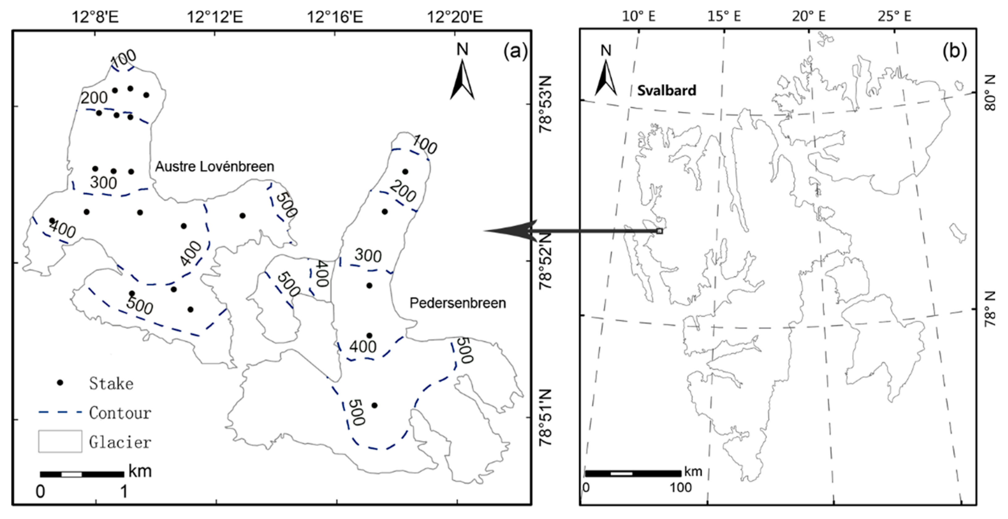
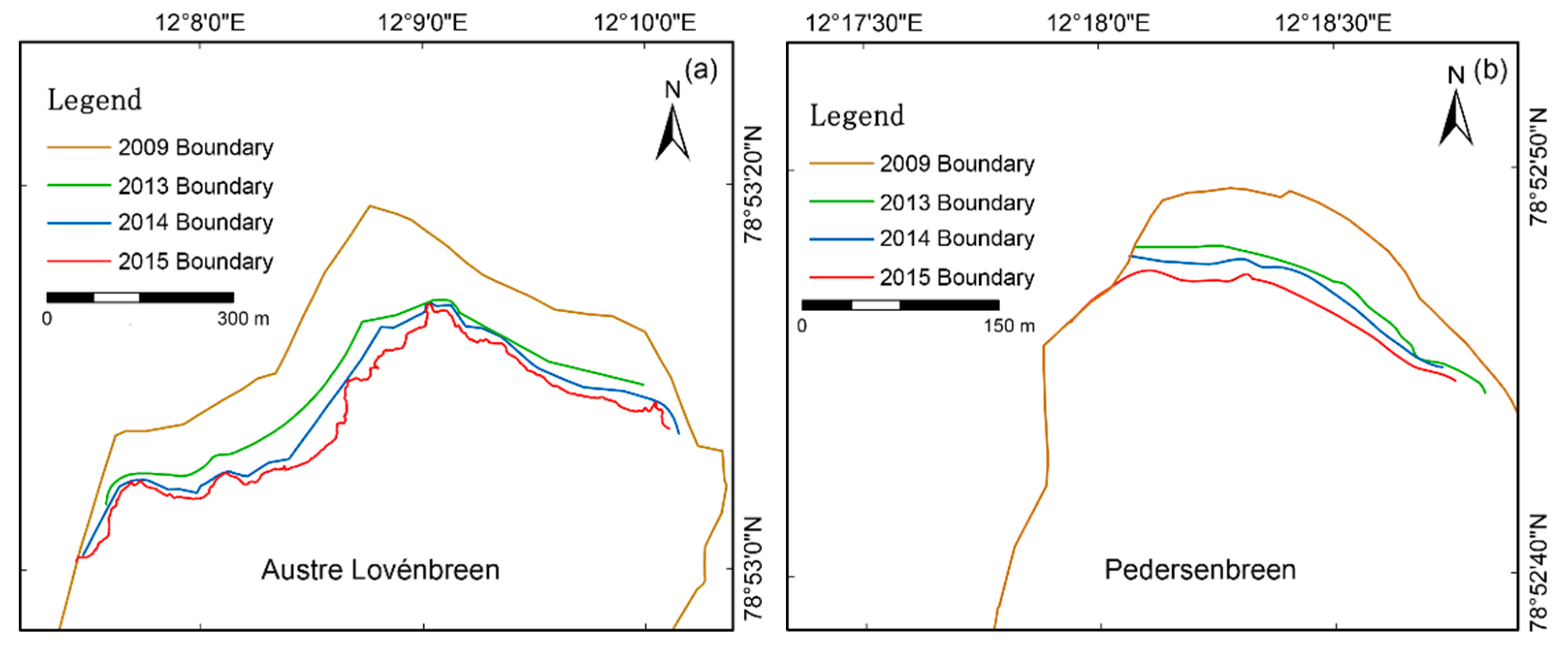
16]. Since the Chinese Arctic Yellow River Station was built in 2004, Chinese researchers have focused on Arctic glaciers, carrying out long-term studies on Austre Lovénbreen and Pedersenbreen in Svalbard [17]. Chinese researchers have investigated the volume of Austre Lovénbreen and Pedersenbreen [18] and estimated the mass loss of Pedersenbreen during the periods from 1936 to 1990 and from 1990 to 2009 [9]. The velocities of the two glaciers have also been studied, and the latest research has discussed the fastest ice flow region of Austre Lovénbreen by combining modeling methods with in situ surveying methods [19].
Since the Little Ice Age (LIA), the glaciers in Svalbard have been retreating. Bamber and others suggested that an increased thinning trend occurred in recent years based on aerial surveys performed in 1996 and 2002 [8]. Małecki concluded that mass changes became more negative in central Svalbard glaciers by comparing elevation changes over the periods 1960–1990 and 1990–2009 [20]. Hagen et al. estimated the annual mass balance for the whole of Svalbard to be −0.1 m water equivalent (w.e.) during the period 1979–2000 [21]. Nuth and others estimated that the annual mass balance of the southern and western Spitsbergen glaciers in Svalbard during the period 1936–1990 was −0.30 m w.e, according to geodetic mass balance estimate from aerial photography [22]. Norwegian researchers observed the mass balance of the two glaciers, Austre Broggerbreen and Midtre Lovenbreen, adjacent to Austre Lovénbreen during the period 1966–1988, finding that the ice surface decreased by 8.9 m and 7.5 m, respectively [14]. A French team comprehensively investigated Austre Lovénbreen, and concluded that the annual mass balance of the glacier during the period 1962–2013 was around −0.2 m w.e., and the annual mass balance in 2008–2015 was about −0.4 m w.e. [
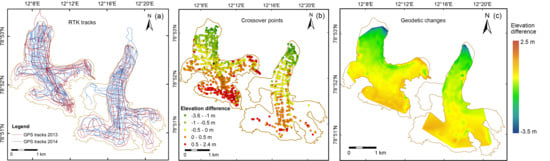
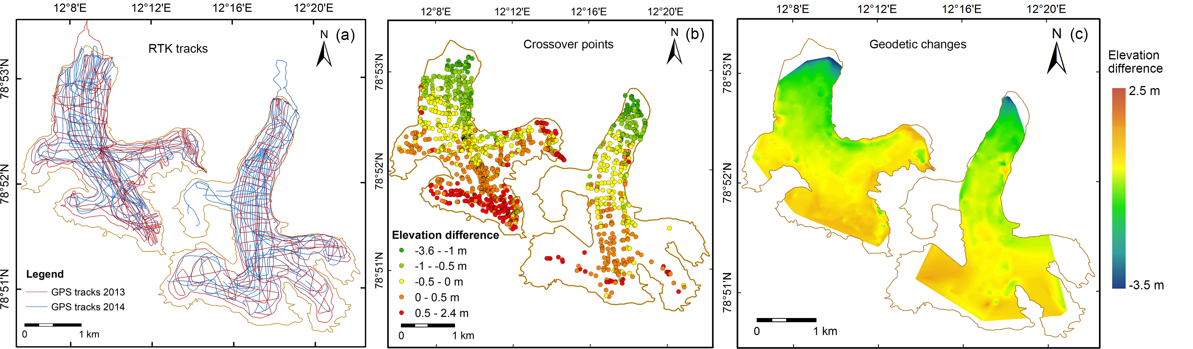
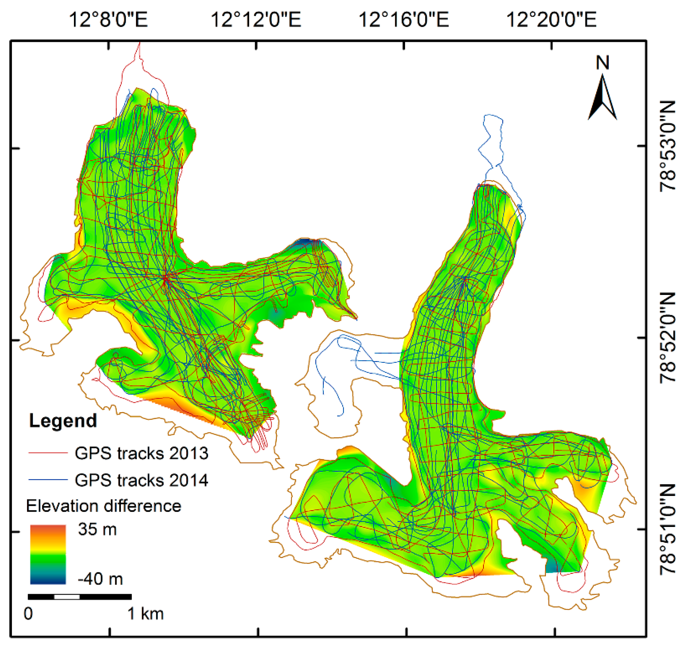
23]. In our study, we mainly used real-time kinematic global positioning system (RTK-GPS) data to map the surface topography and analyze the interannual geodetic mass balance of Austre Lovénbreen and Pedersenbreen via elevation changes, which is of significance as a reference for traditional glacier mass balance estimates.

2. Study Area

The glaciers Austre Lovénbreen (12.09°E; 78.527°N) and Pedersenbreen (12.175°E; 78.515°N) are located in Svalbard in the Arctic (Figure 1) and are 6.2 km and 10 km away from the Chinese Arctic Yellow River Station, respectively. These two glaciers are recognized as polythermal valley glaciers, lying in a mountainous area, with the highest peak reaching 1017 m. Austre Lovénbreen has an area of 4.5 km2 with an altitude between 50 m and 550 m [23]. According to previous research, the glacier valley of Pedersenbreen is V-shaped rather than U-shaped [18], with an area of approximately 5.6 km2 and an altitude between 60 m and 650 m. Pedersenbreen has a narrower snout than Austre Lovénbreen, and both glaciers are relatively flat, and both are covered with small amounts of debris as the elevation increases gradually from the north to the south.
The Svalbard area, where the two glaciers are located, has a polar oceanic type climate mainly affected by the North Atlantic current. This climate is characterized by cooler summers and warmer winters than other regions with similar latitudes [24]. According to the weather station in Ny-Ålesund, where the Chinese Arctic Yellow River Station is located, the annual mean temperature during the past 30 years (1981–2010) was −5.2 °C, with the mean temperatures of 3.8 °C and −12 °C of summer and winter, respectively. The annual average precipitation is 427 mm w.e., which is mainly concentrated in winter and autumn dominated by snow [25]. The annual temperature and precipitation during the earlier period (1961−1990) were −6.3 °C and 385 mm, respectively, indicating that an obvious climate change occurred in the different periods [25]. Overall, the entire archipelago has experienced a warming trend of approximately 0.5 °C every decade since 1960 [26].

3. Data and Methods

3.1. Data

The 20-stake observation network on Austre Lovénbreen and five observation stakes along the central line of Pedersenbreen were placed in July 2005 [27]. The movement of these stakes has been annually monitored with high-precision GPS instruments for glacial movement and mass balance studies [17]. In April 2013, April 2014, and May 2015, high-density RTK-GPS points on the surface of Austre Lovénbreen and Pedersenbreen were collected via a snowmobile carrying GPS equipment, and the GPS tracks are shown in Figure 2. The base station is located at the Yellow River Station in Ny-Ålesund. The main purpose of this survey was to map the surface digital elevation model (DEM) and to estimate surface changes. The height data from the GPS measurements were ellipsoidal heights, which needed to be converted into altitudes above sea level. An elevation benchmark near the glaciers (<10 km) was set in Ny-Ålesund. According to a previous study [18], the geoidal height at this point was calculated as 35.158 m, which was used to convert the measured GPS heights to altitudes above sea level. Because we used the relative change of elevations in this study, the tectonic movement at Ny-Ålesund was neglected, since the two glaciers move together with the earth’s crust motions.
In order to evaluate the quality of the RTK surveys, all crossover points between different RTK profiles in one survey period were picked out, and the height differences of crossover points are shown in Table 1. In general, these small elevation differences proved the relatively high precision of the field surveys in 2013–2015.
Snow cover measurements were performed on Austre Lovénbreen in April of 2013, 2014, and 2015 by a French team working in the area. A Pico drill was used to measure the depth and density of the snow covering the glacier. In addition, ArcticDEM [28] topographic data and ice-surface DEMs of the glacier snouts created by unmanned aerial vehicle (UAV) photogrammetry in 2019 were employed as supplementary data for the investigation of geodetic changes.

3.2. Comparison of Interpolation Methods

Different DEM resolutions have an important impact on ice-surface-elevation change studies [29]. To reveal the impact of different resolutions on the interpolation results and to select a suitable interpolation resolution, we compared different interpolation resolutions, including 0.2 m, 0.5 m, 1 m, 2 m, and 5 m. According to previous studies, interpolation is an important source of uncertainty in mass change studies using DEMs [30,31]. Different interpolation methods need to be compared to determine the most suitable method for generating the DEM. Several widely used interpolation methods were examined—inverse distance weighting (IDW), ordinary kriging (OK), universal kriging (UK), natural neighbor (NN), spline interpolation, and Topo to Raster (TTR) interpolation. IDW determines z-values using a linearly weighted combination of a set of sample points. The influence of known points on the interpolated values, based on their distance from the output point, can be controlled by defining the power. Kriging is an advanced geostatistical procedure that generates an estimated surface from a scattered set of points via z-values; it requires previous exploratory work on input data to determine the parameters that have an important impact on the interpolation results [32]. Two widely used kriging methods are OK and UK. OK assumes that the variation in the z-values is free of drift. UK is a typical geostatistical method that is based on spatial autocorrelation models. It assumes that the spatial variation in the z-values is determined by the drift and a random error [33] and is suitable for data with an obvious trend. The NN approach interpolates a value by finding the closest subset of input samples to an unknown point and applies weights to them based on their proportionate areas [34]. The surface interpolated by splines passes through the input samples and is smooth everywhere except at the locations of the input samples [35]. TTR is based on thin-plate smoothing splines; it creates smooth, continuous surfaces passing through all the input points and aims to produce a raster of the drainage structure [36]. In this study, we selected a spherical model as the semivariogram model for OK, a linear drift model for UK, and a regularized spline for spline interpolation.
In total, 75% of the RTK-GPS points were randomly selected as training data for interpolating the DEM, and the rest were used as testing data. To evaluate the accuracy of the interpolation results, the errors at the testing points were evaluated by subtracting the interpolated values from the ground records of the vertical coordinates. Root mean square errors (RMSEs) were calculated for every interpolation method to assess their performance. All analyses were performed in ArcGIS 10.3 (Environmental Systems Research Institute, United States).

3.3. Estimation of Geodetic Changes

Based on the interpolation results, the optimal interpolation method was chosen for analyzing the interannual geodetic glacier changes. The surface-elevation changes were analyzed by subtracting one DEM from a later DEM. In addition, the trend of geodetic glacier changes was studied in detail by calculating the elevation differences in the crossover points from the RTK-GPS tracks in different years. The mass change research in our study belonged to the geodetic method and was based on real-time kinematic (RTK)-global positioning system (GPS) data, which are advantageous for long-term studies.
If we ignore the influence of ice flux on the mass balance, elevation changes can be converted into geodetic mass balances independent of dynamics [22]. Glacier mass change needs to be transformed from an ice equivalent into a water equivalent, which means that the density of glacial ice and snow should be estimated. Density assumptions or models for converting the geodetic glacier volume change to mass change have been explored in many studies [37,38].
The net geodetic mass balance of a glacier can be calculated from the area-weighted mass balances of different elevation ranges, similar to the traditional mass balance calculation, as in formula (1):
B = i = 1 n B i S i
where B is the net geodetic mass balance, and Bi and Si are the geodetic mass balance at different elevation bins and the corresponding percentage of the projected area between two contour lines, respectively. By calculating the average elevation changes obtained from the crossover points in the different elevation bands, the geodetic mass balance can be obtained with a density model of the ice surface.
For an investigation with such a short time interval, a density model is needed to convert the ice-surface changes in a glacier into the water equivalent for a mass balance study, and in situ snow data are important for estimating the geodetic mass balance. Taking snow depth into consideration, the mass balance at a point can be calculated as in formula (2):
b = Δ h ρ i + ( s 2 s 1 ) ( ρ s ρ i )
where b is the annual mass balance at a given point calculated by the geodetic method (represented by the water equivalent); ∆h is the elevation change; ρi is the ice density (assumed to be 900 kg/m3); ρs is the snow density (assumed to be 400 ± 100 kg/m3); and s1 and s2 represent the snow depths for the first year and the following year, respectively. The snow depth at a given point can be calculated from the interpolation of the snow depth data obtained from in situ snow depth measurements. Accordingly, the mass balances for an entire glacier can be calculated from interpolation.

4. Results

4.1. Comparisons of Different Interpolation Resolutions and Methods

Taking the RTK-GPS data of Pedersenbreen measured in 2013 as an example, we compared the DEMs generated by IDW with spatial resolutions of 0.2 m, 0.5 m, 1 m, 2 m, and 5 m. More than 2800 testing points were used to examine the vertical accuracy of the DEMs derived from the five interpolation resolutions. All the mean errors in Table 2 are close to zero but do not seem to be related to the resolution. However, the quality of the interpolation result was mainly assessed by RMSE (root mean square error). Table 2 illustrated that the RMSE was smaller with a higher resolution, which means that the elevation extracted near the RTK-GPS tracks was more accurate at a higher resolution. Similar conclusions could also be drawn from other interpolation methods at different resolutions.
There were few differences found between the DEMs with resolutions of 0.2 m, 0.5 m, and 1 m based on a comparison of the RMSEs; the differences were at the millimeter level. Considering the limit of the sampling interval of RTK-GPS data, the resolution of the DEM should be appropriate to avoid meaningless interpolation at an over-detailed scale, which would increase the computational burden. Therefore, the final resolution of the DEM in our study was set to 0.5 m. Then, the DEMs generated by different interpolation methods with a resolution of 0.5 m were compared, and the statistics of the errors are shown in Table 3. OK, NN, and spline had similar results; they each had a small RMSE and range, and their mean errors were close to zero, which means that these methods could be considered candidates for generating the DEM. IDW showed the extreme maximum and minimum values and a larger RMSE compared to other methods. The unsatisfied estimation from IDW in this study confirmed the results from other research [39,40]. Although UK had the lowest mean error, the RMSE showed that it was not an optimal method for the surface interpolation of glaciers. TTR had a smaller mean error than NN and spline, but its RMSE was larger than OK, NN, and spline, so we did not consider it when generating the DEMs of the glaciers.
We compared the DEMs generated by OK, NN, and spline interpolation (Figure 3), and the hillshade effect was added to the DEMs to evaluate their smoothness. Although OK produced the lowest RMSE, the surface generated by OK was not as smooth as we would expect, whereas the glacier surface generated by NN interpolation was smooth. The surface generated by spline interpolation had some abnormal regions in which the values varied greatly from the other interpolation results. We selected NN interpolation as the most suitable method for analyzing the surface topography in this study. In fact, there was no single ideal interpolation method for all ice terrains; the interpolation method was chosen according to the terrain topography and the type of data analysis needed.

4.2. Glacier Surface Elevation Changes

The DEMs of the two glacier surfaces in 2013–2015 were derived from NN interpolation. According to the 2013 DEM in Figure 3 the surface DEM of Pedersenbreen generated by NN interpolation is smoother than that of the other interpolation methods, and the lowest elevation is approximately 56 m at the northern part of the glacier terminus. The elevation differences between years were acquired by comparing the DEMs, and the elevation differences between 2013 and 2014 are shown in Figure 4. For Austre Lovénbreen, we subtracted the 2013 DEM from the 2014 DEM and found that the range of the surface-elevation differences was extremely large, as it could not be applied to the range of elevation changes of a glacier in a year; similar results were found for Pedersenbreen. The errors of DEM differences were calculated in Table 4; although the mean errors of the two glaciers seem to indicate possible elevation changes in 2013–2014, and the extremely large ranges in Table 4 are not suitable for interpreting the range of elevation changes. The spatial distribution of the elevation differences in Figure 4. is not in accordance with the fact that ice elevations do not change drastically over such a short time interval, assuming the glacier is in a steady state. This discrepancy is ascribed, in part, to the data source of the DEM, as the abnormal regions are mainly distributed at edges with steep topography that do not have GPS tracks in either 2013 or 2014. A similar result was also obtained by comparing the DEMs in other years.
The RTK-GPS points measured in 2013–2015 were not dense enough to cover the entire glacier, resulting in abnormal elevation difference values at certain regions where the RTK-GPS points were sparse. Misleading elevation change results might be obtained by DEM comparisons. Therefore, an alternative method was proposed: calculate the elevation difference in the crossover points from the RTK-GPS tracks in different years, where the glacier surface changes could be partly revealed by those points.
We derived the boundaries of the two glaciers in 2013–2015, as shown in Figure 5. Considering the retreat of the glacier terminus beginning in 2009, and to ensure that we studied the crossover points in glaciated regions, some crossover points located in the glacier terminus were removed according to their boundaries, and the remaining points were used to study the elevation changes.
The elevation differences in the crossover points of the RTK-GPS tracks from different years in the glaciated regions are shown in Figure 6. From 2013 to 2014, the elevation differences ranged from −2.3 to 1.7 m in the study region (Austre Lovénbreen and Pedersenbreen), and the values of most points were negative. From 2014 to 2015, the elevation difference in the two glaciers was −2.0 to 1.9 m, and the values of most points were positive. By observing the distribution of elevation difference at the crossover points, we found that the trend in the elevation difference was more obvious than that calculated by the DEM. The elevation difference gradually increased from north to south, and its value changed from negative to positive. Combined with glacier topography, the altitude had an important impact on elevation changes because elevation changes were negative in most regions with lower altitudes. Higher altitude regions had a less negative elevation change, and, at even higher regions, the elevation increased. In general, the elevations in high-altitude regions were increasing, and the elevations in low-altitude regions were decreasing.
We derived a continuous raster of the elevation differences using NN interpolation (Figure 7), and the results illustrated that there was a good relationship between the change in elevation and the corresponding elevation of the two glaciers. In the figure, the color gradient corresponds to the elevation.
The regional distribution of the surface-elevation change is obvious. Austre Lovénbreen and Pedersenbreen experienced significant losses at their terminuses. However, there were some obvious regions of accumulation at the lower elevations of Austre Lovénbreen, such as the western margin area and the eastern tributary margins. Pedersenbreen also exhibited an obvious accumulation region at a relatively low elevation (at the eastern margin), which was mainly due to the mass compensation caused by an avalanche around the edge of the glacier in 2015. These regions are marked in Figure 8. There was an ablation region at the east margin of Austre Lovénbreen (marked with the number 4), which was probably caused by an avalanche that occurred in 2013 but not in 2015, which caused the extremely high elevation measured in 2013. Based on the hillshade topography of the Arctic DEM around the glacier (Figure 8), we found that the mass flow path corresponded to the elevation change area at the edges of the glaciers where slopes were steep.

4.3. Geodetic Glacier Mass Balances

The average annual changes in different elevation bands were obtained from the crossover points, and the results are shown in Table 5. For Austre Lovénbreen, the surface elevation of the entire glacier covered 100–600 m, while Pedersenbreen covered a larger elevation range of about 60–650 m. As shown in the table, there was an obvious relationship between mass change and elevation. The elevation changes in low-altitude areas were negative, indicating that these areas were thinning, and the elevation changes in high-altitude areas were positive, where mass accumulated. In addition, the mass changes varied greatly in different years. In 2013–2014, except for a small amount of accumulation above 500 m, the elevation in most areas of the two glaciers decreased, and the two glaciers seemed to have experienced widespread mass loss. During 2014–2015, the mass accumulation of both glaciers occurred above 300 m, and both glaciers seemed to have a positive mass balance.
The snow depth and density of the two glaciers were not completely recorded in this study, and it was difficult to estimate the precise mass density of the glaciers. Therefore, we tentatively used the elevation changes to indicate geodetic changes over the years. In our study, using the elevation changes at different elevation bins as Bi (the geodetic mass balance at different elevation bins) according to formula (1), together with the data in Table 5, we calculated different years’ geodetic changes, which were actually the mean surface elevation changes of the two glaciers, as shown in Table 6.
According to Table 6, Austre Lovénbreen and Pedersenbreen experienced various mass changes in different years. The mass balance was negative in 2013–2014, while it was positive in 2014–2015, but the geodetic balance in 2013–2015 was not completely in accordance with the sum of the mass balances from 2013–2014 and 2014–2015. However, the bias was at the centimeter level, meeting the error level threshold we anticipated. In addition, some differences could be obtained from comparisons; for example, in 2013–2015, Austre Lovénbreen experienced a more serious mass loss than Pedersenbreen, which experienced a mass gain.
To illustrate the relationship between elevation changes and the surface elevation more directly, scatterplots are shown in Figure 9. There appeared to be a significant correlation between the elevation and the elevation change in 2013–2015. In general, both glaciers showed that the correlation was slightly lower in one-year intervals than in a two-year interval. The correlation at the glacier snout differed from the correlation for the entire glacier area; the ice melted more dramatically in the glacier snouts at elevations between 100 m and 200 m, according to the elevation change trend. According to Figure 9, the mass loss trend of Austre Lovénbreen was more dramatic than that of Pedersenbreen. This finding was consistent with the mass balance results in Table 6.
We evaluated the trends of the surface-elevation changes in different years. The corresponding equilibrium line altitudes (ELAs) of Austre Lovénbreen in 2013–2014, 2014–2015, and 2013–2015 were 490 m, 287 m, and 375 m, respectively, and the ELAs of Pedersenbreen in 2013–2014, 2014–2015, and 2013–2015 were 550 m, 285 m, and 385 m, respectively. Shifts in the ELA are often considered to be good indicators for assessing glacial imbalances and estimating mass budget changes [41]. The ELAs in our study differed greatly in different years, and the long-term ELA seemed to be a more reliable indicator. According to the French team, the average ELA of Austre Lovénbreen in 2008–2014 was 431 m [23]. The annual elevation gradient of the geodetic mass balance of Austre Lovénbreen in 2013–2015 was 2.60‰, which means that in the accumulation region, the accumulation increased by 260 mm for every increase of 100 m in the elevation. In contrast, in the ablation area, the ablation increased by 260 mm for every decrease of 100 m in elevation. Accordingly, the annual elevation gradient of the geodetic mass balance of Pedersenbreen was 2.35‰.
Estimating the mass balance of a glacier must consider changes in the entire area; however, field surveys can cover most regions of glaciers, except for high-elevation regions and margins where the slopes are steep. Therefore, in no-data regions, especially at the margin of the glacier snout where the ice melts quickly, it is necessary to make an appropriate estimate of the mass change value. At glacier snouts, the elevation changes need to be corrected. According to the relationship between elevation changes and the elevation (Figure 9), the elevation change from 100 to 200 m for Austre Lovénbreen and the elevation change from 60 to 200 m for Pedersenbreen could be corrected. Some previous studies have made density assumptions of 900 kg/m3 in the ablation area, and 500 to 600 kg/m3 in the accumulation area, dominated by firn [15,37,42,43]. If we ignore short-term changes in the vertical firn density, we can assume that the density of the glacier surface is 900 kg/m3 in the ablation area and 500 kg/m3 in the accumulation zone when converting elevation changes into mass balances, represented by their water equivalents. Finally, the geodetic mass balances of Austre Lovénbreen and Pedersenbreen in 2013–2014, 2014–2015, and 2013–2015 are shown in Table 7. Because winter snow accumulation in Svalbard does not vary greatly between years, the mass changes of glaciers are mainly dominated by the melting of snow and ice in summer [44]. If we assume that snowfall is invariable, in our study, the geodetic balance in 2013–2014 should be approximately equal to the mass balance in 2013 calculated by the glaciological method, and the geodetic balance in 2014–2015 should be close to the actual mass balance in 2014.

5. Discussion

There are some factors that may influence the accuracy of mass-balance assessments. We let April to April of the next year be a balance year for the mass balance study, while September to September of the next year is usually considered a hydrological year in the Arctic in the classic glaciological method. Different survey time-spans may lead to some discrepancies in comparisons with the glaciological method. Taking Austre Lovénbreen as an example, the net mass balances computed by the French team were −1.111 m w.e. in 2013, 0.010 m w.e. in 2014, and −0.552 m w.e. in 2015 [23]. According to the mass balance obtained by the French team, the geodetic mass balance of Austre Lovénbreen in 2013–2014 in Table 7 should be approximately equal to the sum of the summer mass balance in 2013 and the winter mass balance in 2014. In addition, the geodetic mass balance in 2014–2015 should be close to the sum of the summer mass balance in 2014 and the winter mass balance in 2015. However, our study appeared to underestimate the mass loss in 2013, which might be partly ascribed to ignoring snow depth. On the other hand, it is difficult to calculate the mass balance accurately by a simple linear simulation, as the elevation changes in the lateral zones of the glacier are smaller than the change in the glacier’s center [22], and the classic glaciological method may not consider potential subglacier mass changes. Although there may be some discrepancies, the mass balance change trend in our study was consistent with the trend calculated by the French team, which means that the method proposed here to calculate the geodetic mass balance is valid. Similar geodetic methods with high-density GPS data were also applied to other regions. Repeated differential GPS surveys were carried out on Gangju La glacier, Bhutan Himalaya; the annual and decadal geodetic mass balances calculated from the GPS points and snow depth showed consistency with the direct mass balance observed from stakes [6]. Marinsek and Ermolin compared the elevation differences from kinematic GPS surveys on Bahía del Diablo glacier on the Antarctic Peninsula in 2000–2001 and 2010, finding that the geodetic mass balance calculated based on elevation change was close to the glaciological mass balance [45].
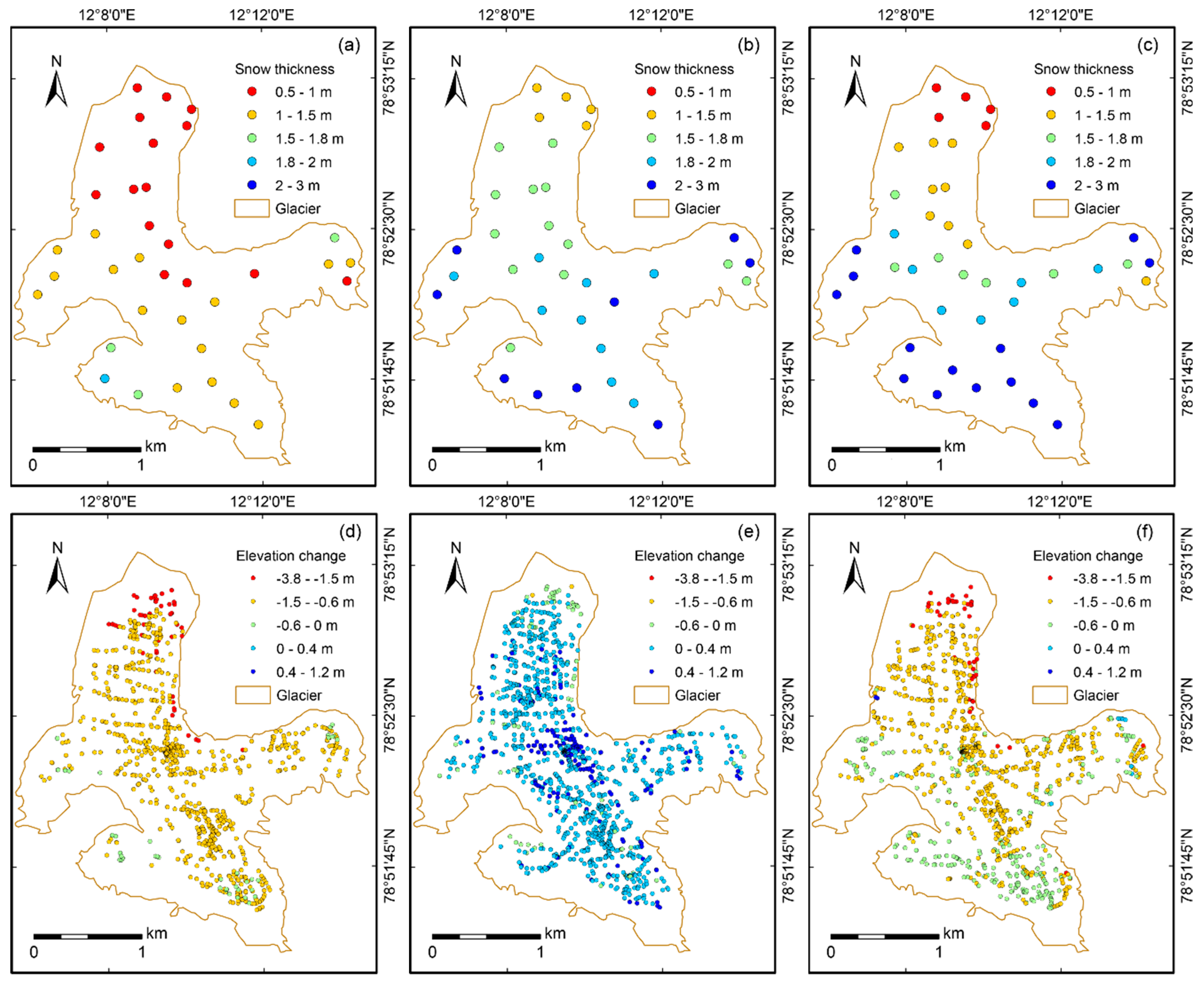
Snow depth data of Austre Lovénbreen were obtained from the French team for validation and comparison over the same period (during 2013–2015). The snow depth distributions of Austre Lovénbreen (Figure 10a–c) demonstrated that the snow depth logically increased from north to south, with shallower snow depths at lower elevations and more snow accumulation at higher elevations, representing a positive relationship between snow depth and elevation. According to Figure 10d–f, more snow remained because of glacial accumulation in 2014 than in the other two years combined. In addition, Austre Lovénbreen experienced similar snow accumulation at relatively low elevations in 2013 and 2015, even though 2013 was shallower; in contrast, in the upper cirques of the glacier, there was clearly a deeper snow depth in 2015 than in the two other years. This situation was in accordance with the analyses we performed with RTK-GPS data; hence, we believed that the main difference between 2014 and 2015 was that the snow at relatively high elevations in 2014 did not melt completely during the melting season. In contrast, very little snow survived the summer of 2013, and little or no accumulation was observed. To accurately calculate the mass balance of Austre Lovénbreen, the interpolated snow depths in three years measured by snow cores were removed from the crossover points of the RTK-GPS tracks. Then, ice-surface elevation changes were calculated, as shown in Figure 10d–f. In conjunction with snow depth, the ice changes and snow changes were calculated separately.
According to formula (2), the mass balances of crossover points in different years could be calculated; in addition, the mass balances for the entire glacier could be calculated from natural neighbor interpolation. As the previous study suggested, the density of the winter snowpack was between 350 and 450 kg m−3 for the Austfonna ice cap, Svalbard [46]. With the assumed ice density of 900 kg/m3 and the assumed snow density of 350 kg/m3 in this study, the mass changes in the crossover points of the RTK-GPS tracks were estimated with the ice changes and snow changes and then interpolated, as shown in Figure 11. For the region without data, an appropriate approximation of average mass balance was performed by extracting the mass balance values in the surrounding areas covered by the mass balance interpolation results, and the corresponding area percentages of the no-data regions and data covered region were calculated. Then, the mass balances of the entire glacier were estimated from the area-weighted mass balances; the results are shown in Table 8. The mass balance of Austre Lovénbreen in 2013–2014, shown in Table 8, was close to −0.760 m w.e., which was the sum of the summer mass balance in 2013 and the winter mass balance in 2014. The mass balance in 2014–2015 was close to 0.136 m w.e, which was the glaciological mass balance recorded by the French team over the same period. Although some discrepancies still exist in comparison with the actual observation results, the mass balance results calculated when considering snow depth seemed to be more reasonable than those calculated while ignoring snow depth.
There was a large mass loss ascribed to ice melting in 2013. However, the deeper snow in 2014 compensated for the elevation change, leading us to underestimate the ice loss. To explain this phenomenon more directly, we estimated the geodetic mass balance without snow depth data at a point with formula (3):
b = Δ h ρ
where b is the mass balance, ∆h is the elevation change, and ρ is the estimated average density of the ice and snow mixture. If formula (2) and formula (3) are both true, and the elevation change is not 0 m, then the relationship between the assumed average density and the snow depth can be obtained as formula (4):
ρ = ρ i + ( s 2 s 1 ) ( ρ s ρ i ) / Δ h
where ρi is the ice density; ρs is the snow density; and s1 and s2 represent the snow depths for the first year and the following year, respectively. The snow density and ice density are assumed to be invariant. Taking the years of 2013 and 2014 as an example, s2 is far larger than s1, and ∆h is less than 0 m in most regions; hence, only when the average density ρ is larger than the ice density ρi, we can obtain the correct geodetic mass balance. We usually assume the average density to be less than the ice density. However, over a relatively long time interval, the elevation change is considerable, and the snow depth can be neglected in comparison with the ice change; thus, the mass balance can be more accurately calculated with the elevation change data. In fact, over a short time interval, the results of the density assumption are inconsistent with the results obtained, considering limited volumetric changes [37]. This means that, ignoring snow depth, which varied greatly during our research period, might have resulted in a larger bias in the mass balance over a short time interval.
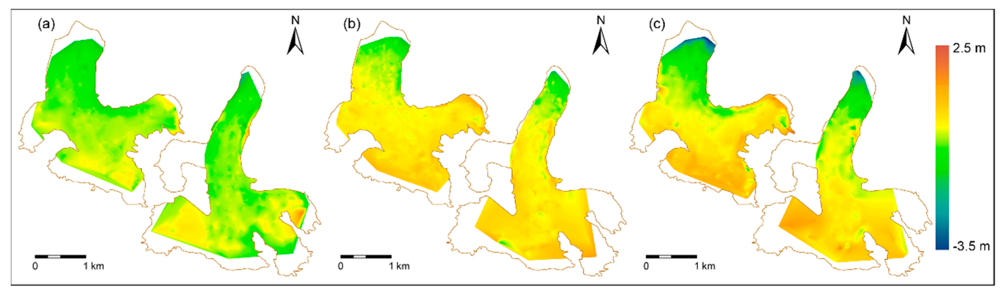
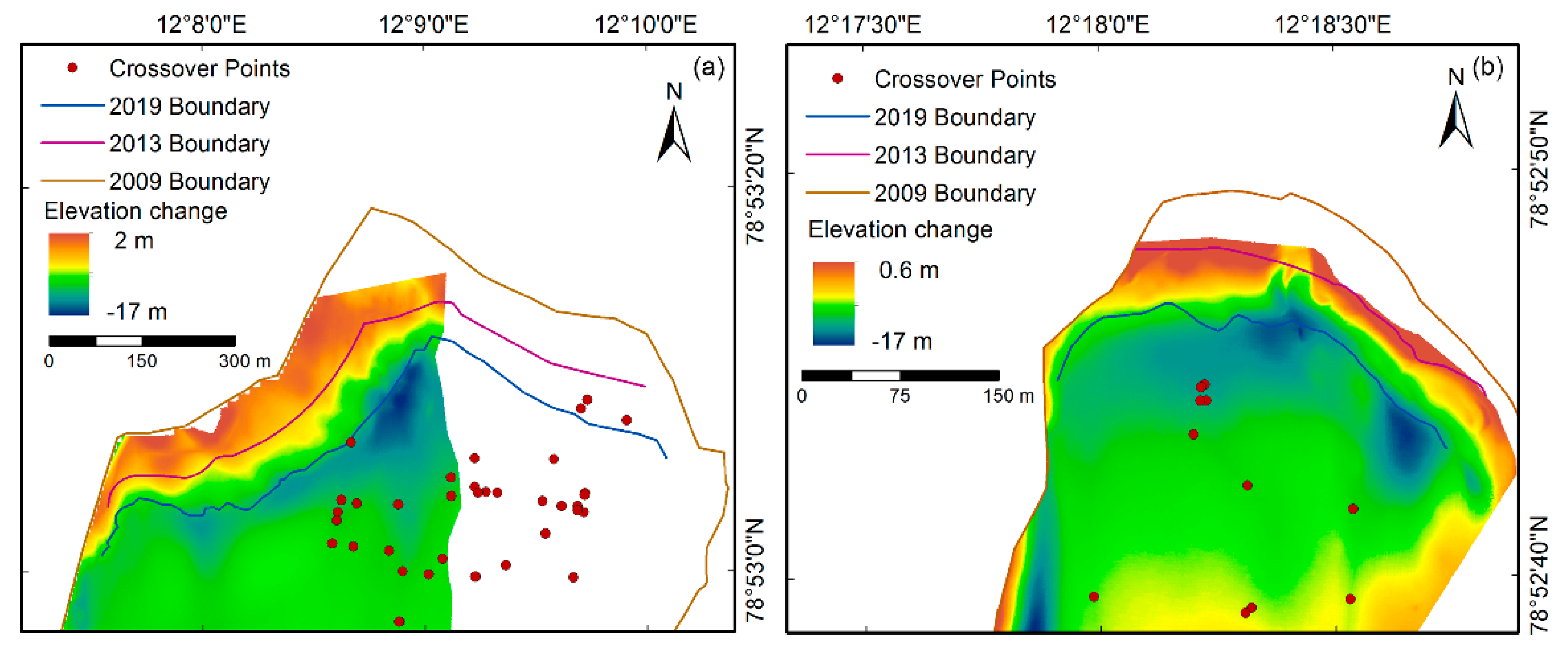
Using a UAV-generated DEM of glacier snout in 2019, we calculated the elevation differences of the glacier snouts between 2013 and 2019 by comparing the DEMs of different years; the results are shown in Figure 12, according to which the two glacier snouts experienced serious mass loss from 2013 to 2019, and the elevation decreased by 17 m in maximum. In order to precisely compare the elevation changes, we only extracted the 2019 surface elevations at crossover points whose positions were derived from RTK-GPS tracks in 2013 and 2015 (Figure 12). At these specific point locations, inside the 2019 DEM coverage, the mean elevation changes in different years were calculated as in Table 9. Although the 2019 DEM covered only the snout area of each glacier, the point elevation changes presented a clear tendency from 2013 to 2019. The mean value of elevation changes in 2015–2019 was two to three times as much as that in 2013–2015, which proved that both glaciers are in an accelerating thinning situation, at least over their snout areas.
In this study, we evaluated the smoothness and accuracy of the interpolated glacier surface using different methods, and NN was finally chosen for our RTK-GPS data interpolation. However, the optimum interpolation method depends on the characteristics of the source data, the complexity of the terrain, and the desired properties of the interpolated result. Therefore, we need to evaluate the interpolation methods cautiously in other instances. The terrain itself, the density, and the uncertainty of input data are also important factors in choosing interpolation methods. For example, NN interpolation will ignore details of the terrain, which fits well with glacier surfaces but may not be suitable for complex terrains. Accuracy and smoothness are usually our desired properties. However, the little experience can be obtained from previous studies. For instance, kriging was applied to analyze the mass balance of Storglaciären [47]. Some researchers have used IDW to create a continuous surface of thickness values along the branch lines at the bed of a glacier [48]. In other studies, spline interpolation was chosen to generate the DEM of Alpine glaciers [49]. Bo and others used NN interpolation to build regional DEMs within the Antarctic ice sheet [50]. Mölg concluded that Kriging and Topo to Raster showed robust and reliable results in a mass balance study on the Conejeras glacier, Colombia [51]. Pellitero and others presented a semi-automated method to generate ice thickness from bed topography along a palaeoglacier flowline by applying the standard flow law for ice and generating the 3D surface of the palaeoglacier using multiple interpolation methods, in which IDW and kriging performed well in volume estimation [52]. Kääb chose spline, kriging, and IDW approaches to interpolate surface elevation changes along contour lines on the Svalbard glacial Edgeøya, and the volume change estimations using three interpolation methods were similar [53].
To widely interpret the trends in the geodetic mass balance distribution of Arctic glaciers, we compared the elevation changes and the geodetic mass balance of Austre Lovénbreen and Pedersenbreen. They experienced similar geodetic mass balances: a serious mass loss in 2013–2014 and a slight mass accumulation in 2014–2015. Nevertheless, some differences can be noted, as Austre Lovénbreen displayed stronger thinning than Pedersenbreen. The elevation range distribution of these two glaciers may explain this difference [17] because the area percentage of Pedersenbreen in higher altitude regions is larger than Austre Lovénbreen.
In addition, high-density RTK-GPS measurements require considerable in situ work, considering the complexity of RTK-GPS surveys. Therefore, surveys were only carried out in 2013, 2014, and 2015. Due to this limited time, the mass change results may not be completely consistent with the long-term trends; we found that geodetic balances varied greatly in 2013–2015. For a short-term trend, there seems to be some uncertainty in estimating mass balances by the geodetic method, which requires caution when converting the elevation changes estimated with RTK-GPS data into mass balances. Long-term RTK-GPS data covering the entire glaciers are required for additional comprehensive analyses, which would contribute to future comparative studies with the glaciological method.

6. Conclusions

Based on RTK-GPS data, the surface-elevation changes and the geodetic mass balances of Austre Lovénbreen and Pedersenbreen were preliminarily studied. The following conclusions could be drawn from our analysis.
(1)
We compared different interpolation methods, and NN interpolation was more suitable for generating the surface DEMs of glaciers.
(2)
The elevation changes across different years were estimated both by the differences in the DEMs and the differences in the RTK-GPS track-derived crossover point elevations; the latter was more suitable for estimating elevation changes linked to the corresponding altitude.
(3)
Ignoring the effect of snow depth over a short time interval might lead to a larger bias in the mass balance, especially when the snow of the following year is far deeper than that of the first year during a negative balance period. However, for a study spanning a long time interval (more than 10 years), the snow depth could be neglected in comparison with the ice change. Therefore, caution must be exercised when estimating mass balances with elevation change data from only a few years, and the mass balances estimated with RTK-GPS data might be more accurate for investigations over a longer time interval.
(4)
The average ELA and the annual elevation gradient of the geodetic mass balance of Austre Lovénbreen in 2013–2015 were 375 m and 2.60‰, respectively, and those of Pedersenbreen were 385 m and 2.35‰, respectively. The gradients of the two glaciers were three times larger at the glacier snouts, according to the elevation changes at the crossover points from the RTK-GPS tracks. In the study period, Austre Lovénbreen experienced a more serious mass loss than Pedersenbreen, and both glaciers were in accelerating thinning status at snout areas.

Author Contributions

S.A. and Z.W. conceived the study and supervised the experiments. X.D. and F.T. wrote the manuscript. X.D. and X.Z. processed some data and produced some of the figures. S.A., Z.W., and F.T. contributed to the field data collection on the glaciers.

Funding

This research was funded by the National Natural Science Foundation of China (41531069, 41476162).

Acknowledgments

Our study was supported by the National Natural Science Foundation of China (41531069, 41476162). The field data in this article were acquired by researchers from the Chinese Arctic Yellow River Station. We thank the Chinese Arctic and Antarctic Administration of the State Oceanic Administration for sponsoring the field expeditions around the Chinese Arctic Yellow River Station. Snow cover data were acquired by the French team with the support of the French Polar Institute (IPEV) and the French Agence Nationale de la Recherche (ANR). We are grateful to the team members who supported our in situ observations.

Conflicts of Interest

The authors declare that they have no conflicts of interest to disclose.

References

  1. Haeberli, W.; Hoelzle, M.; Paul, F.; Zemp, M. Integrated monitoring of mountain glaciers as key indicators of global climate change: The European Alps. Ann. Glaciol. 2007, 46, 150–160. [Google Scholar] [CrossRef] [Green Version]
  2. Paul, F.; Bolch, T.; Kaab, A.; Nagler, T.; Nuth, C.; Scharrer, K. The glaciers climate change initiative: Methods for creating glacier area, elevation change and velocity products. Remote Sens. Environ. 2015, 162, 408–426. [Google Scholar] [CrossRef] [Green Version]
  3. Nuth, C.; Moholdt, G.; Kohler, J.; Hagen, J.O.; Kaab, A. Svalbard glacier elevation changes and contribution to sea level rise. J. Geophys. Res. Earth Surf. 2010, 115. [Google Scholar] [CrossRef] [Green Version]
  4. Larsen, C.F.; Motyka, R.J.; Arendt, A.; Echelmeyer, K.A.; Geissler, P.E. Glacier changes in southeast Alaska and northwest British Columbia and contribution to sea level rise. J. Geophys. Res. Earth Surf. 2007, 112. [Google Scholar] [CrossRef]
  5. Braithwaite, R.J. Glacier mass balance: The first 50 years of international monitoring. Prog. Phys. Geogr. 2002, 26, 76–95. [Google Scholar] [CrossRef]
  6. Tshering, P.; Fujita, K. First in situ record of decadal glacier mass balance (2003–2014) from the Bhutan Himalaya. Ann. Glaciol. 2016, 57, 289–294. [Google Scholar] [CrossRef] [Green Version]
  7. Woul, M.D.; Hock, R. Static mass-Balance sensitivity of arctic glaciers and ice caps using a degree-Day approach. Ann. Glaciol. 2005, 42, 217–224. [Google Scholar] [CrossRef] [Green Version]
  8. Bamber, J.L.; Krabill, W.; Raper, V.; Dowdeswell, J.A.; Oerlemans, J. Elevation changes measured on Svalbard glaciers and ice caps from airborne laser data. Ann. Glaciol. 2005, 42, 202–208. [Google Scholar] [CrossRef] [Green Version]
  9. Ai, S.; Wang, Z.; Tan, Z.; E, D.C.; Yan, M. Mass change study on Arctic glacier Pedersenbreen, during 1936–1990–2009. Chin. Sci. Bull. 2013, 58, 3148–3154. [Google Scholar] [CrossRef] [Green Version]
  10. Wang, P.; Li, Z.; Li, H.; Wang, W.; Yao, H. Comparison of glaciological and geodetic mass balance at Urumqi glacier No. 1, Tian Shan, Central Asia. Global Planet. Change 2014, 114, 14–22. [Google Scholar] [CrossRef]
  11. Cox, L.H.; March, R.S. Comparison of geodetic and glaciological mass-Balance techniques, Gulkana Glacier, Alaska, USA. J. Glaciol. 2004, 50, 363–370. [Google Scholar] [CrossRef] [Green Version]
  12. Paul, F.; Haeberli, W. Spatial variability of glacier elevation changes in the Swiss Alps obtained from two digital elevation models. Geophys. Res. Lett. 2008, 35. [Google Scholar] [CrossRef] [Green Version]
  13. Fischer, A. Comparison of direct and geodetic mass balances on a multi-annual time scale. Cryosphere 2011, 5, 107–124. [Google Scholar] [CrossRef] [Green Version]
  14. Hagen, J.O.; Liestol, O. Long-Term glacier mass-balance investigations in Svalbard, 1950–1988. Ann. Glaciol. 1990, 14, 102–106. [Google Scholar] [CrossRef] [Green Version]
  15. Moholdt, G.; Nuth, C.; Hagen, J.O.; Kohler, J. Recent elevation changes of Svalbard glaciers derived from ICESat laser altimetry. Remote Sens. Environ. 2010, 114, 2756–2767. [Google Scholar] [CrossRef]
  16. Hagen, J.O.; Eiken, T.; Kohler, J.; Melvold, K. Geometry changes on Svalbard glaciers: Mass-Balance or dynamic response. Ann. Glaciol. 2005, 42, 255–261. [Google Scholar] [CrossRef] [Green Version]
  17. Xu, M.; Yan, M.; Ren, J.; Ai, S.; Kang, J.; E, D.C. Surface mass balance and ice flow of the glaciers Austre Lovenbreen and Pedersenbreen, Svalbard, Arctic. Chin. J. Pol. Sci. 2010, 21, 147–159. [Google Scholar]
  18. Ai, S.; Wang, Z.; E, D.; Holmen, K.; Tan, Z.; Zhou, C.; Sun, W. Topography, ice thickness and ice volume of the glacier Pedersenbreen in Svalbard, using GPR and GPS. Pol. Res. 2014, 33, 18533. [Google Scholar] [CrossRef] [Green Version]
  19. Ai, S.; Ding, X.; An, J.; Lin, G.; Wang, Z.; Yan, M. Discovery of the Fastest Ice Flow along the Central Flow Line of Austre Lovenbreen, a Poly-Thermal Valley Glacier in Svalbard. Remote Sens. 2019, 11, 1488. [Google Scholar] [CrossRef] [Green Version]
  20. Malecki, J. Elevation and volume changes of seven Dickson Land glaciers, Svalbard, 1960–1990–2009. Pol. Res. 2013, 32, 18400. [Google Scholar] [CrossRef]
  21. Hagen, J.O.; Melvold, K.; Pinglot, F.; Dowdeswell, J.A. On the net mass balance of the glaciers and ice caps in Svalbard, Norwegian Arctic. Arct. Antarc. Alpine Res. 2003, 35, 264–270. [Google Scholar] [CrossRef] [Green Version]
  22. Nuth, C.; Kohler, J.; Aas, H.F.; Brandt, O.; Hagen, J.O. Glacier geometry and elevation changes on Svalbard (1936-90): A baseline dataset. Ann. Glaciol. 2007, 46, 106–116. [Google Scholar] [CrossRef] [Green Version]
  23. Marlin, C.; Tolle, F.; Griselin, M.; Bernard, E.; Saintenoy, A.; Quenet, M.; Friedt, J.M. Change in geometry of a high Arctic glacier from 1948 to 2013 (Austre Lovenbreen, Svalbard). Geogr. Ann. Ser. A Phys. Geogr. 2017, 99, 115–138. [Google Scholar] [CrossRef]
  24. Moller, M.; Finkelnburg, R.; Braun, M.; Hock, R.; Jonsell, U.; Pohjola, V.A.; Scherer, D.; Schneider, C. Climatic mass balance of the ice cap Vestfonna, Svalbard: A spatially distributed assessment using ERA-Interim and MODIS data. J. Geophys. Res. 2011, 116. [Google Scholar] [CrossRef] [Green Version]
  25. Forland, E.J.; Benestad, R.; Hanssen-Bauer, I.; Haugen, J.E.; Skaugen, T.E. Temperature and Precipitation Development at Svalbard 1900–2100. Adv. Meteorol. 2011, 2011, 1–14. [Google Scholar] [CrossRef]
  26. Nowak, A.; Hodson, A. Changes in meltwater chemistry over a 20-Year period following a thermal regime switch from polythermal to cold-Based glaciation at Austre Broggerbreen, Svalbard. Pol. Res. 2014, 33, 22779. [Google Scholar] [CrossRef] [Green Version]
  27. Ai, S.; E, D.; Yan, M.; Ren, J. Arctic glacier movement monitoring with GPS method on 2005. Chin. J. Pol. Sci. 2006, 17, 61–68. [Google Scholar]
  28. Porter, C.; Morin, P.; Howat, I.; Noh, M.J.; Bates, B.; Peterman, K.; Keesey, S.; Schlenk, M.; Gardiner, J.; Willis, M.; et al. “ArcticDEM”. Harv. Dataverse 2018, 1. [Google Scholar] [CrossRef]
  29. Gardelle, J.; Berthier, E.; Arnaud, Y. Impact of resolution and radar penetration on glacier elevation changes computed from DEM differencing. J. Glaciol. 2012, 58, 419–422. [Google Scholar] [CrossRef] [Green Version]
  30. Zemp, M.; Thibert, E.; Huss, M.; Stumm, D.; Rolstad, C.; Nuth, C.; Nussbaumer, S.U.; Moholdt, G.; Mercer, A.; Mayer, C. Reanalysing glacier mass balance measurement series. Cryosphere 2013, 7, 1227–1245. [Google Scholar] [CrossRef] [Green Version]
  31. Rolstad, C.; Haug, T.; Denby, B. Spatially integrated geodetic glacier mass balance and its uncertainty based on geostatistical analysis: Application to the western Svartisen ice cap, Norway. J. Glaciol. 2009, 55, 666–680. [Google Scholar] [CrossRef] [Green Version]
  32. Oliver, M.A.; Webster, R. A tutorial guide to geostatistics: Computing and modelling variograms and kriging. Catena 2014, 113, 56–69. [Google Scholar] [CrossRef]
  33. Armstrong, M. Problems with universal kriging. Math. Geol. 1984, 16, 101–108. [Google Scholar] [CrossRef]
  34. Guo, Q.; Li, W.; Yu, H.; Alvarez, O. Effects of topographic variability and lidar sampling density on several DEM interpolation methods. Photogramm. Eng. Remote Sens. 2010, 76, 701–712. [Google Scholar] [CrossRef] [Green Version]
  35. Bojanov, B.D.; Hakopian, H.A.; Sahakian, A.A. Spline Functions and Multivariate Interpolations; Kluwer: Norwell, MA, USA, 1993. [Google Scholar]
  36. Hutchinson, M.F. A new procedure for gridding elevation and stream line data with automatic removal of spurious pits. J. Hydrol. 1989, 106, 211–232. [Google Scholar] [CrossRef]
  37. Huss, M. Density assumptions for converting geodetic glacier volume change to mass change. Cryosphere 2013, 7, 877–887. [Google Scholar] [CrossRef] [Green Version]
  38. Kaab, A.; Treichler, D.; Nuth, C.; Berthier, E. Brief communication: Contending estimates of 2003–2008 glacier mass balance over the Pamir–Karakoram–Himalaya. Cryosphere 2015, 9, 557–564. [Google Scholar] [CrossRef] [Green Version]
  39. Erdogan, S. A comparision of interpolation methods for producing digital elevation models at the field scale. Earth Surf. Process. Landf. 2009, 34, 366–376. [Google Scholar] [CrossRef]
  40. Racoviteanu, A.E.; Manley, W.F.; Arnaud, Y.; Williams, M.W. Evaluating digital elevation models for glaciologic applications: An example from Nevado Coropuna, Peruvian Andes. Global Planet. Change 2007, 59, 110–125. [Google Scholar] [CrossRef]
  41. Huss, M.; Dhulst, L.; Bauder, A. New long-Term mass-Balance series for the Swiss Alps. J. Glaciol. 2016, 61, 551–562. [Google Scholar] [CrossRef] [Green Version]
  42. Kaab, A.; Berthier, E.; Nuth, C.; Gardelle, J.; Arnaud, Y. Contrasting patterns of early twenty-First-Century glacier mass change in the Himalayas. Nature 2012, 488, 495–498. [Google Scholar] [CrossRef]
  43. Gardelle, J.; Berthier, E.; Arnaud, Y. Slight mass gain of karakoram glaciers in the early twenty-First century. Nat. Geosci. 2012, 5, 322–325. [Google Scholar] [CrossRef]
  44. Hagen, J.O.; Kohler, J.; Melvold, K.; Winther, J.G. Glaciers in Svalbard: Mass balance, runoff and freshwater flux. Pol. Res. 2003, 22, 145–159. [Google Scholar] [CrossRef] [Green Version]
  45. Marinsek, S.; Ermolin, E. 10 year mass balance by glaciological and geodetic methods of Glaciar Bahia del Diablo, Vega Island, Antarctic Peninsula. Ann. Glaciol. 2015, 56, 141–146. [Google Scholar] [CrossRef] [Green Version]
  46. Dunse, T.; Schuler, T.; Hagen, J.; Eiken, T.; Brandt, O.; Hogda, K. Recent fluctuations in the extent of the firn area of Austfonna, Svalbard, inferred from GPR. Ann. Glaciol. 2009, 50, 155–162. [Google Scholar] [CrossRef] [Green Version]
  47. Hock, R.; Jensen, H. Application of kriging interpolation for glacier mass balance computations. Geogr. Ann. Ser. A Phys. Geogr. 1999, 81, 611–619. [Google Scholar] [CrossRef]
  48. Paul, F.; Linsbauer, A. Modeling of glacier bed topography from glacier outlines, central branch lines, and a DEM. Int. J. Geogr. Inf. Sci. 2012, 26, 1173–1190. [Google Scholar] [CrossRef]
  49. Mennis, J.L.; Fountain, A.G. A spatio-Temporal GIS database for monitoring alpine glacier change. Photogramm. Eng. Remote Sens. 2001, 67, 967–975. [Google Scholar]
  50. Bo, S.; Siegert, M.J.; Mudd, S.M.; Sugden, D.; Fujita, S. The Gamburtsev mountains and the origin and early evolution of the Antarctic Ice Sheet. Nature 2009, 459, 690–693. [Google Scholar] [CrossRef]
  51. Molg, N.; Ceballos, J.L.; Huggel, C.; Micheletti, N.; Rabatel, A.; Zemp, M. Ten years of monthly mass balance of Conejeras glacier, Colombia, and their evaluation using different interpolation methods. Geogr. Ann. Ser. A Phys. Geogr. 2017, 99, 155–176. [Google Scholar] [CrossRef]
  52. Pellitero, R.; Rea, B.R.; Spagnolo, M.; Bakke, J.; Ivy-Ochs, S.; Frew, C.R.; Hughes, P.; Ribolini, A.; Lukas, S.; Renssen, H. GlaRe, a GIS tool to reconstruct the 3D surface of palaeoglaciers. Comput. Geosci. 2016, 94, 77–85. [Google Scholar] [CrossRef] [Green Version]
  53. Kaab, A. Glacier Volume Changes Using ASTER Satellite Stereo and ICESat GLAS Laser Altimetry. A Test Study on Edgeoya, Eastern Svalbard. IEEE Trans. Geosci. Remote Sens. 2008, 46, 2823–2830. [Google Scholar] [CrossRef]
Figure 1. (a) Sketch view of Austre Lovénbreen and Pedersenbreen and (b) the locations of the glaciers in Svalbard.
Remotesensing 11 02890 g001
Figure 2. Real-time kinematic global positioning system (RTK-GPS) tracks in different years: (a) 2013, (b) 2014, and (c) 2015.
Remotesensing 11 02890 g002
Figure 3. DEMs (digital elevation models) of Pedersenbreen in 2013 generated from different interpolation methods: (a) OK (ordinary kriging), (b) NN (natural neighbor) interpolation, and (c) spline interpolation.
Remotesensing 11 02890 g003
Figure 4. Elevation differences in 2013–2014.
Remotesensing 11 02890 g004
Figure 5. Glacier boundaries of (a) Austre Lovénbreen and (b) Pedersenbreen.
Remotesensing 11 02890 g005
Figure 6. Elevation differences in the crossover points of the RTK-GPS (real-time kinematic global positioning system) tracks from different years: (a) 2013–2014, (b) 2014–2015, and (c) 2013–2015.
Remotesensing 11 02890 g006
Figure 7. Elevation differences in different years interpolated with the crossover points: (a) 2013–2014, (b) 2014–2015, and (c) 2013–2015.
Remotesensing 11 02890 g007
Figure 8. Hillshade topography and elevation changes for Austre Lovénbreen (left) and Pedersenbreen (right) from 2013 to 2015. The dashed ellipse marked regions represent ablation areas (green color, number 4) and accumulation areas (red color, number 1, 2, 3, 5) near the margins of the glaciers.
Remotesensing 11 02890 g008
Figure 9. Scatterplot of the ice-surface elevations versus the surface-elevation changes (unit: m) for Austre Lovénbreen (ac) and Pedersenbreen (df) in different years.
Remotesensing 11 02890 g009
Figure 10. Spatial distributions of snow depth observed in (a) 2013, (b) 2014, and (c) 2015 and ice-surface elevation changes in the crossover points of the RTK-GPS (real-time kinematic global positioning system) tracks after removing the snow depth of Austre Lovénbreen in (d) 2013–2014, (e) 2014–2015, and (f) 2013–2015.
Remotesensing 11 02890 g010
Figure 11. Mass balances calculated considering the snow depth of Austre Lovénbreen in (a) 2013–2014, (b) 2014–2015, and (c) 2013–2015.
Remotesensing 11 02890 g011
Figure 12. Elevation changes for the glacier snouts of (a) Austre Lovénbreen and (b) Pedersenbreen from 2013 to 2019. The 2019 boundaries of two glaciers were extracted from UAV (unmanned aerial vehicle) images. The crossover points were extracted from RTK-GPS (real-time kinematic global positioning system) tracks between 2013 and 2015.
Remotesensing 11 02890 g012
Table 1. Elevation differences of the crossover points between different RTK (real-time kinematic) profiles. The Mean and RMSE (root mean square error) are the primary indicators for data quality evaluation.
Austre LovénbreenPedersenbreen
YearCountRMSEMaxMeanCountRMSEMaxMean
20133320.078 m0.779 m−0.020 m1430.080 m0.313 m−0.007 m
20145730.061 m0.582 m0.002 m5270.080 m0.437 m0.000 m
20157660.097 m1.147 m−0.011 m3070.077 m0.367 m0.004 m
Table 2. Errors in the IDW (inverse distance weighting) interpolation results with different resolutions (unit: m).
0.2 m0.5 m1 m2 m5 m
Mean0.0040.0350.021−0.035−0.023
RMSE0.3590.3630.3660.3930.444
Max4.0964.1584.1063.6314.104
Min−2.425−2.385−2.582−2.951−2.648
Range6.5216.5436.6886.5826.752
Table 3. Errors in different interpolation methods (unit: m).
IDWOKUKNNSplineTTR
Mean0.0350.0240.0110.0280.0290.027
RMSE0.3620.0920.2140.0950.0990.187
Max4.1580.71671.3450.6940.7251.567
Min−2.385−0.687−1.418−0.721−0.714−1.690
Range6.5431.4042.7631.4151.4393.257
IDW, OK, UK, NN, and TTR are abbreviations of inverse distance weighting, ordinary kriging, universal kriging, natural neighbor interpolation, and Topo to Raster interpolation, respectively.
Table 4. DEM (digital elevation model) differences in 2013–2014 (unit: m).
Austre LovénbreenPedersenbreen
Mean−0.379 −0.202
STD4.555 3.654
Min−41.714 −30.047
Max30.042 34.976
Range71.756 65.023
Table 5. Elevation changes for Austre Lovénbreen and Pedersenbreen at different elevation intervals (unit: m).
GlacierYear<200200–300300–400400–500≥500
Austre Lovénbreen2013–2014−0.919−0.560−0.253−0.0970.007
2014–2015−0.528−0.0840.2160.4890.562
2013–2015 −1.594 −0.622 −0.052 0.418 0.520
Pedersenbreen2013–2014 −0.833−0.403−0.311−0.1950.027
2014–2015 −0.4890.0660.2580.3670.445
2013–2015 −1.375−0.336−0.0920.2020.532
Table 6. Surface elevation changes in 2013–2015 (unit: m).
YearAustre LovénbreenPedersenbreen
2013–2014 −0.279 −0.164
2014–2015 0.236 0.309
2013–2015 −0.055 0.172
Table 7. Geodetic mass balances in 2013–2015 after correction (unit: m w.e. (water equivalent)).
YearAustre LovénbreenPedersenbreen
2013–2014−0.267 −0.165
2014–20150.079 0.129
2013–2015−0.165 0.012
Table 8. The geodetic mass balances for Austre Lovénbreen calculated with and without consideration of snow depth and the mass balance calculated by the glaciological method over the same period (unit: m w.e. (water equivalent)).
YearIgnoring Snow DepthConsidering Snow DepthGlaciological Mass Balance
2013–2014−0.267 −0.670−0.760
2014–20150.079 0.184 0.136
2013–2015−0.165 −0.490 −0.624
Table 9. Mean elevation changes of crossover points at glacier snout areas from 2013 to 2019 (unit: m/a).
YearAustre LovénbreenPedersenbreen
2013–2015 −0.75 −1.19
2015–2019 −2.23 −2.26
2013–2019 −1.73−1.90

