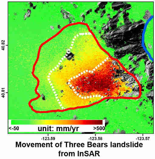
Characterization of the Kinematics of Three Bears Landslide in Northern California Using L-band InSAR Observations

Abstract

High-precision monitoring of landslides is essential for understanding their kinematics and reducing landslide induced damage. The spatiotemporal deformation variations of the Three Bears landslide in northern California have not been systematically monitored and interpreted. In this study, we applied advanced time-series InSAR analysis methods to characterize the kinematics of the landslide covering two periods (2007–2011 and 2015–2017) with multi-track synthetic aperture radar (SAR) images acquired from L-band ALOS PALSAR-1/2 satellites. Our results show that the Three Bears landslide has been moving consistently, with the Line of Sight (LOS) deformation rate exceeding 300 mm/yr from 2007 to 2011 and around 250 mm/yr from 2015 to 2017. The east–west and vertical deformation components were inverted by integrating ascending and descending ALOS PALSAR-2 interferograms during the 2015–2017 period, indicating that the landslide was dominated by eastward movement and in a continuous deformation stage. Down-slope landslide motions observed from adjacent satellite tracks with slightly different radar look vectors were used to verify the accuracy of InSAR-derived results. Comparison between linearly detrended InSAR displacements and precipitation records indicate that the landslide tends to accelerate during the wet seasons. The results could allow us to better understand the kinematics of the landslide and provide significant evidence for evaluating the potential for catastrophic failure and the threat posed by such failure to human life and property. Combined with a proper geotechnical/geomechanical model, the results would also facilitate the design and implementation of mitigation measures.

1. Introduction

Landslides constitute one of the most frequent and serious natural hazards in mountainous areas around the world, and can be triggered by various factors such as rainfall or snowmelt, earthquakes and human activities [1,2]. Therefore, long-term monitoring of slope instability is key to understanding the kinematic mechanisms of landslide movement as well as reducing landslide induced damage. Many different surveying methods such as inclinometers, piezometers, photogrammetry, and global positioning system (GPS) have been employed to monitor landslides [3,4,5,6]. However, some of these methods are spatially-limited, time-consuming, and logistically challenging. Optical remote sensing techniques can also be used to monitor landslide movement, however, it is often difficult to obtain the pre- and post-slide optical images as the quality of images depends on the cloud cover and identifiable textural features. In general, optical imagery is always effective at monitoring shallow rapid landslides that strip away vegetation and scour channels, but less so for tracking deep-seated landslide movements, which often have a negligible effect on vegetation. Tracking landslide processes can be achieved if high-resolution drone images or ground-based photogrammetry are available [7]. In recent years, interferometric synthetic aperture radar (InSAR) techniques have shown great potentials for monitoring active landslides in remote regions due to the advantages of all-day, all-weather, wide coverage, and high spatial resolution, especially with the successive launch of SAR satellites and the great abundance of SAR images [8,9,10,11,12,13,14].

The Three Bears landslide at Cedar Grove Ranch in northern California is located on the west side of the South Fork Trinity River and is about 8.05 km south of its junction with the main stem (Figure 1a). It is about 4.19 km long and 0.97 km wide, and the toe terminates on the South Fork Trinity River. The most active part appears to be the lower third of the feature, immediately above the river (Figure 1b) [15]. It is situated predominantly within a north–south trending band of weak Rattlesnake Creek Terrane rocks, made up of a mélange of Paleozoic marine sedimentary and metasedimentary rocks. Detailed geologic units are described in Figure S1 in the Supplementary Materials. The proximity to the Cascadia subduction zone makes this area prone to strong ground shaking, with peak ground accelerations in the order of 25–30% of gravity forces, which are likely to influence the activity of the landslide [15]. The activity of the Three Bears landslide can be seen in the oldest available aerial photographs from 1944 [15]. Then, a large discrete landslide was identified in the vicinity of Cedar Grove Ranch by the California Department of Water Resources in 1979 [16]. Zhao et al. [10] only detected the location and approximate boundary of the Three Bears landslide with ALOS PALSAR-1 InSAR imagery from 2007 to 2011. However, the spatiotemporal evolution of landslide movement is rarely recorded and almost unknown to the public. Here, we utilize advanced time-series InSAR techniques [17,18,19], along with L-band ALOS PALSAR-1 (2007–2011) and ALOS PALSAR-2 (2015–2017) datasets, to reveal the spatial extent and temporal kinematic behavior of the Three Bears landslide and further compare the InSAR-derived measurements with the meteorological records to better understand the landslide motion in response to precipitation.

2. Data

The study area, located in the mountainous region of northern California, is covered by dense vegetation. In order to better characterize the kinematic behavior of the landslide’s movement, a total of 66 L-band SAR scenes acquired from six different datasets were collected. The detailed parameters for these six datasets are listed in

Table 1. The detailed parameters of the synthetic aperture radar (SAR) datasets used in this study.

Sensor	ALOS PALSAR-1		ALOS PALSAR-2
Path	223	224	68	69	170	171
Orbital direction	ascending	ascending	ascending	ascending	descending	descending
Heading (°)	‒10.18	‒9.83	‒10.88	‒9.73	‒170.17	–169.01
Incidence angle (°)	37.52	40.18	30.45	40.63	39.60	29.22
Number of scenes	19	21	6	6	7	7
Acquisition period (yyyymmdd)	20070314–20110325	20070213–20110109	20150210–20171114	20140914–20171105	20150525–20171023	20150307–20171111

, while their coverages are shown in Figure 1a. One-arc-second digital elevation model (DEM) data with a resolution of 30 m, generated by Shuttle Radar Topography Mission (SRTM) [20], was adopted to simulate and remove the topographic phase in the interferometric processing.

Since the ALOS PALSAR-1 satellite was launched in May 2006, the perpendicular baselines of the interferograms increased almost linearly during the first two years. Then, an orbit maneuver was conducted in July 2008 with a baseline shift of about 5000 m for P223 (Figure 2a) and for P224 (Figure 2b). Thus, to reduce the artifact induced by the large baseline on the interferograms [21], the general strategy for time-series analysis based on ALOS PALSAR-1 images is to avoid the use of the SAR data acquired during the summer of 2008 [22], which results in a disconnected interferometric baseline network. To bridge the gap caused by the orbit maneuver in July 2008, we chose interferograms with a perpendicular baseline within 2000 m and a temporal baseline within 1000 days. After removing the interferometric pairs with low coherence, twenty-six interferograms for P223 (Figure 2a) and fifty interferograms for P224 (Figure 2b) were finally selected to conduct the following time-series InSAR analysis.

In light of the sparse temporal sampling of ALOS PALSAR-2 data in the study area, all available SAR images were used to generate the interferograms without the spatial and temporal baseline constraints. Although the perpendicular baselines of interferograms were smaller than those from the ALOS PALSAR-1 data, the quality of the interferograms was also strongly influenced by the large deformation gradient and temporal decorrelation. After removing the interferometric pairs with poor coherence, seven interferograms for P68 (Figure 2c), four interferograms for P69 (Figure 2d), fourteen interferograms for P170 (Figure 2e), and eleven interferograms for P171 (Figure 2f) were used to estimate the average deformation velocity and time-series displacements of the landslide.

C-band Envisat ASAR and Sentinel-1A/B data were also processed to obtain the landslide deformation. Unfortunately, a large deformation gradient and thick vegetation make it difficult to sustain good coherence and provide useful signals on this densely vegetated landslide (Figure 1c).

3. Methodology

Depending on the number of available SAR images, two advanced time-series InSAR analysis methods were employed to characterize the kinematic behavior of landslide movement. Furthermore, two-dimensional deformations were retrieved by fusing the measurements from both ascending and descending satellites in the same period.

3.1. Interferometric Point Target Analysis (IPTA)

Interferometric point target analysis (IPTA) is a time-series InSAR technique that provides multiple strategies for the identification of point target candidates, spatial/temporal phase unwrapping, and single- or multi-patch regression analysis processing [18,23].

In light of the large deformation gradient and dense vegetation cover in our study area, multi-master interferograms were considered to maximize the coherence. First, we applied the spectral diversity of Single Look Complex (SLC) images to identify the point target candidates based on the fact that the backscattering intensity of a point target remains almost stable in the case of different fractional azimuth and range bandwidths [18]. To better separate point targets in the dense vegetated areas, the pixels with a coherence value larger than 0.3 were chosen as an initial point target candidate. Then, we iteratively retrieved the linear deformation component and the DEM error of point target candidates based on the wrapped differential interferometric phases using a two-dimensional regression analysis model. Followed by temporal and spatial filtering to the residual unwrapped phases, the nonlinear deformation component and atmospheric artifact are finally separated. Thus, the non-linear time-series deformation of each point target can be obtained by calculating the sum of linear and nonlinear deformation components.

3.2. Small Baseline Subsets (SBAS)

Due to the limited interferometric sets from the ALOS PALSAR-2 satellite, the small baseline subsets (SBAS) InSAR technique [17,24,25] was applied to retrieve the landslide deformation. To obtain the DEM error and time-series deformation, a refined SBAS-InSAR method was applied in our study, which divides the interferograms into high- and low-quality sets and estimates the parameters iteratively [26]. It is worth noting that the accuracy of the InSAR-derived results depends on the quality of the unwrapped interferograms. In general, a minimum cost flow (MCF) method with the aid of coherence is adopted to unwrap the interferogram [27]. However, the continuous motion of the Three Bears landslide makes it troublesome to produce effective long-duration (>70 days) interferograms (Figure 3a). Therefore, a deformation model constructed from a stack of correctly-unwrapped short-duration interferograms (Figure 3b) was introduced and then subtracted from the original interferogram. Thus, we could maintain coherence and minimize the phase unwrapping error. After the residual interferometric phase was filtered and unwrapped, the subtracted deformation derived from the deformation model was added back into the residual unwrapped interferogram (Figure 3c). This technique works well because it prevents the phase gradient of adjacent pixels exceeding $\pi$ radian (5.9 cm for ALOS PALSAR-2). We carefully compared the new unwrapped interferograms (Figure 3c) with the original wrapped interferograms (Figure 3a) to ensure that no artifacts were introduced in this processing. Once the interferograms were successfully unwrapped, the time series deformation could be readily retrieved by using either the least squares (LS) or a singular value decomposition (SVD) method.

3.3. Two-Dimensional Time-Series Inversion with Multi-Track SAR Datasets

The SAR data from each independent track were processed using the above-mentioned IPTA or SBAS, so the InSAR observations were limited to the LOS ascending or descending direction. The availability of ascending and descending ALOS PALSAR-2 measurements in the Three Bears landslide provides us with an opportunity to extend the displacement vectors to 2-D or 3-D [28]. Theoretically, the three-dimensional (3-D) deformation can be retrieved by integrating InSAR observations acquired from at least three independent LOS directions [28,29]. However, since the current SAR satellites are operated in the near-polar orbits, which are insensitive to the north–south movement, the displacement in the north–south direction can hardly be accurately estimated just based on the ascending and descending right-looking InSAR measurements. For ALOS PALSAR-2 datasets listed in Table 1, the contributions of the three (north–south, east–west, and vertical) components to the LOS direction were about 9–11%, 48–64%, and 76–87%, respectively. Therefore, the north–south deformation contribution can be neglected to some extent [19]. Thus, only the east–west and vertical deformation components were simultaneously inverted by using a multidimensional small baseline subset (MSBAS) InSAR technique [19,30].

Considering that all interferograms from $K$ independent SAR imaging geometries have been correctly unwrapped and resampled into a common geographic coordinate system, then the two-dimensional time-series inversion model can be formulated as the following form:

$$\left(\begin{array}{cc}-\frac{4\pi }{{\lambda }^1}{U}_e^1{A}^1& -\frac{4\pi }{{\lambda }^1}{U}_u^1{A}^1\\ -\frac{4\pi }{{\lambda }^2}{U}_e^2{A}^2& -\frac{4\pi }{{\lambda }^2}{U}_u^2{A}^2\\ \cdots & \cdots \\ -\frac{4\pi }{{\lambda }^K}{U}_e^K{A}^K& -\frac{4\pi }{{\lambda }^K}{U}_u^K{A}^K\end{array}\right)\left(\begin{array}{c}{v}_{e,1}\\ ⋮\\ v_{e,N}\\ v_{u,1}\\ ⋮\\ v_{u,N}\end{array}\right)=\left(\begin{array}{c}{\Phi }^1\\ {\Phi }^2\\ \cdots \\ {\Phi }^K\end{array}\right)$$

(1)

where $A$ is the coefficient matrix composed of the time intervals of two consecutive SAR images and $N+1$ represents the number of all of the available SAR images; $\left\{U_e,U_u\right\}=\left\{-\cos \alpha \sin \theta ,\cos \theta \right\}$ is the east–west and vertical components; $\alpha$ and $\theta$ are the azimuth and incidence angles, respectively; $v_e$ and $v_u$ are the unknown east–west and vertical deformation rates that are to be estimated, which represent the deformation rate between the two adjacent SAR acquisitions $t_i$ and $t_{i+1}$; and $\Phi$ denotes the observed unwrapped phases. It can be clearly seen that the design matrix in Equation (1) is rank-deficient because there are no available connections among the InSAR observations from independent imaging geometries. Therefore, SVD method and Tikhonov regularization operator were simultaneously adopted to solve the unknown deformation rates [19] and the east–west and vertical time-series deformation are readily reconstructed by integrating the computed deformation rates.

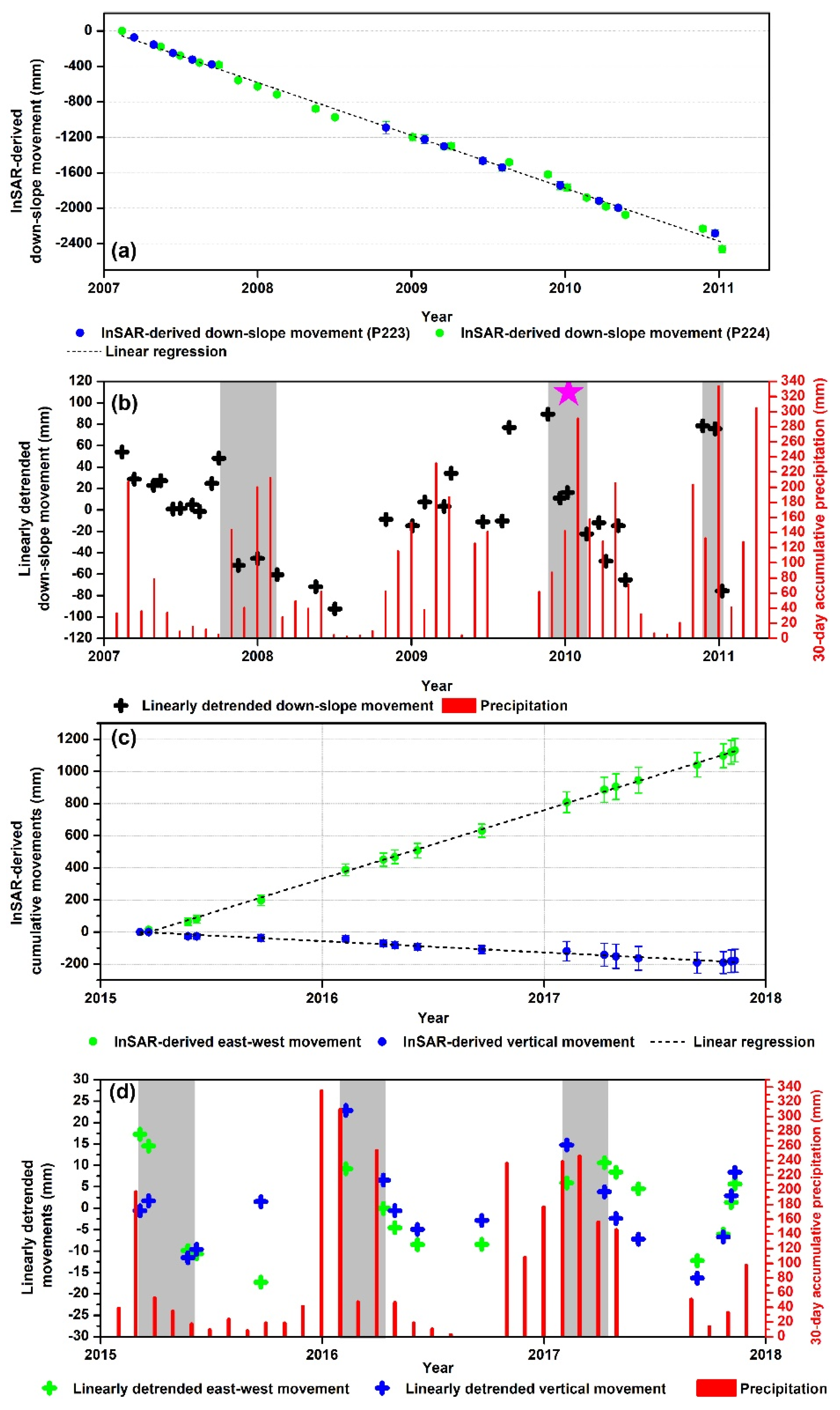
3.4. Deformation in the Down-Slope Direction

Only the projection of the three-dimensional ground deformation along the LOS direction can be obtained using InSAR technique. However, most of the sliding motion generally occurs in the down-slope direction (e.g., [31]). With some assumption, the LOS deformation can be transferred to the slope direction determined by a specific slope angle and azimuth direction. In this work, we projected the LOS measurements to the down-slope direction and then verified the InSAR-derived results based on the overlapping observations from independent satellite tracks.

The transformation from the radar LOS direction to down-slope direction can be easily implemented with the following amplification/scaling factor (e.g., [11,32]):

$$A=1/(l\ast s^T)$$

(2)

where $l=[\begin{array}{ccc}\sin \theta \sin \alpha & -\sin \theta \cos \alpha & \cos \theta \end{array}]$ is the unit vector of the LOS direction, while $s=[-\begin{array}{ccc}\cos \beta \cos \gamma & -\cos \beta \sin \gamma & \sin \beta \end{array}]$ is the unit vector of the down-slope direction, in which $\beta$ and $\gamma$ are the slope angle and slope aspect, respectively.

4. Results

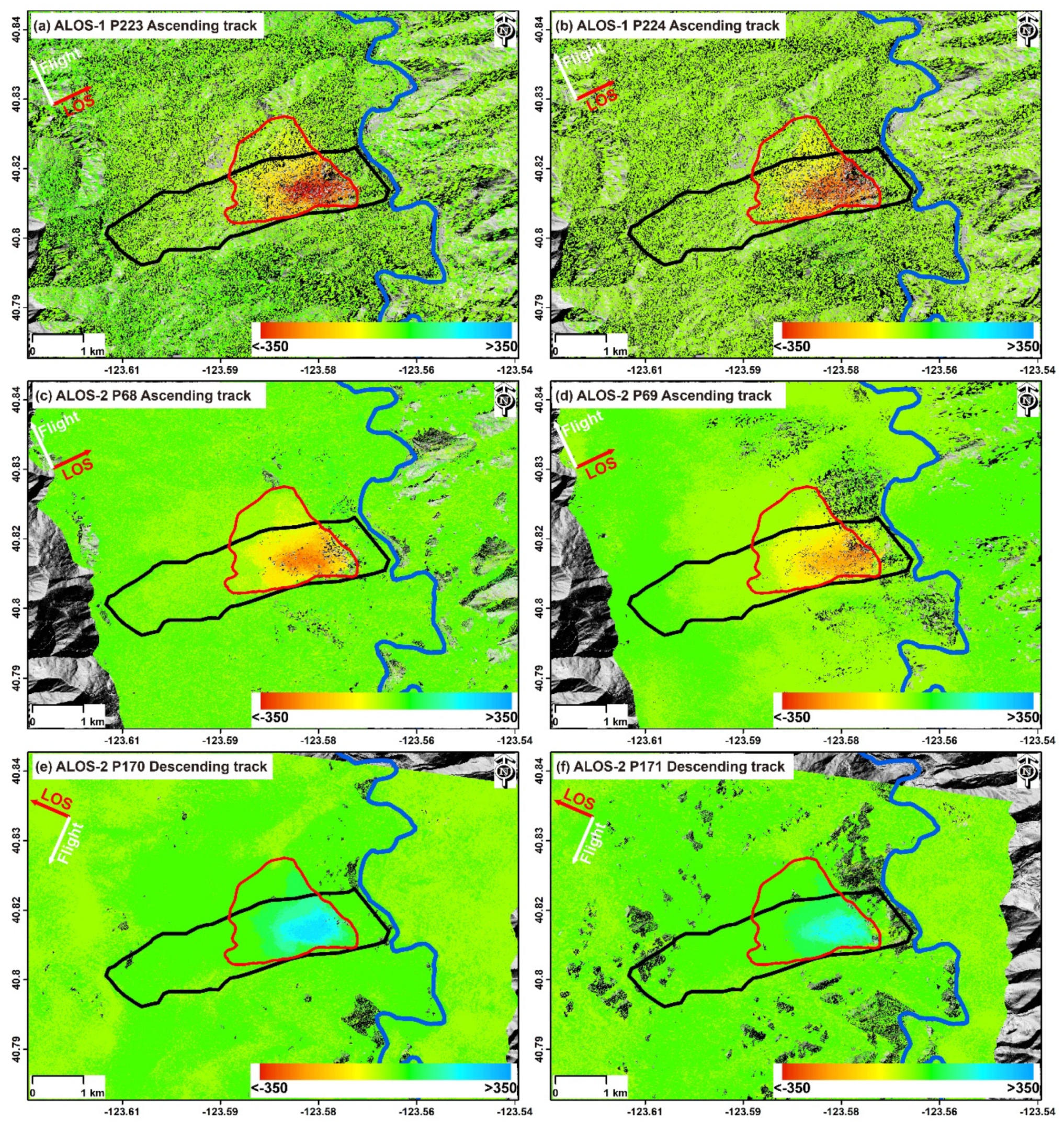
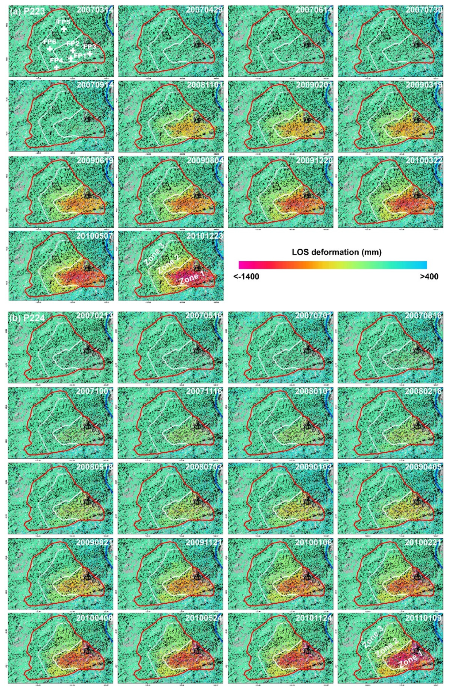
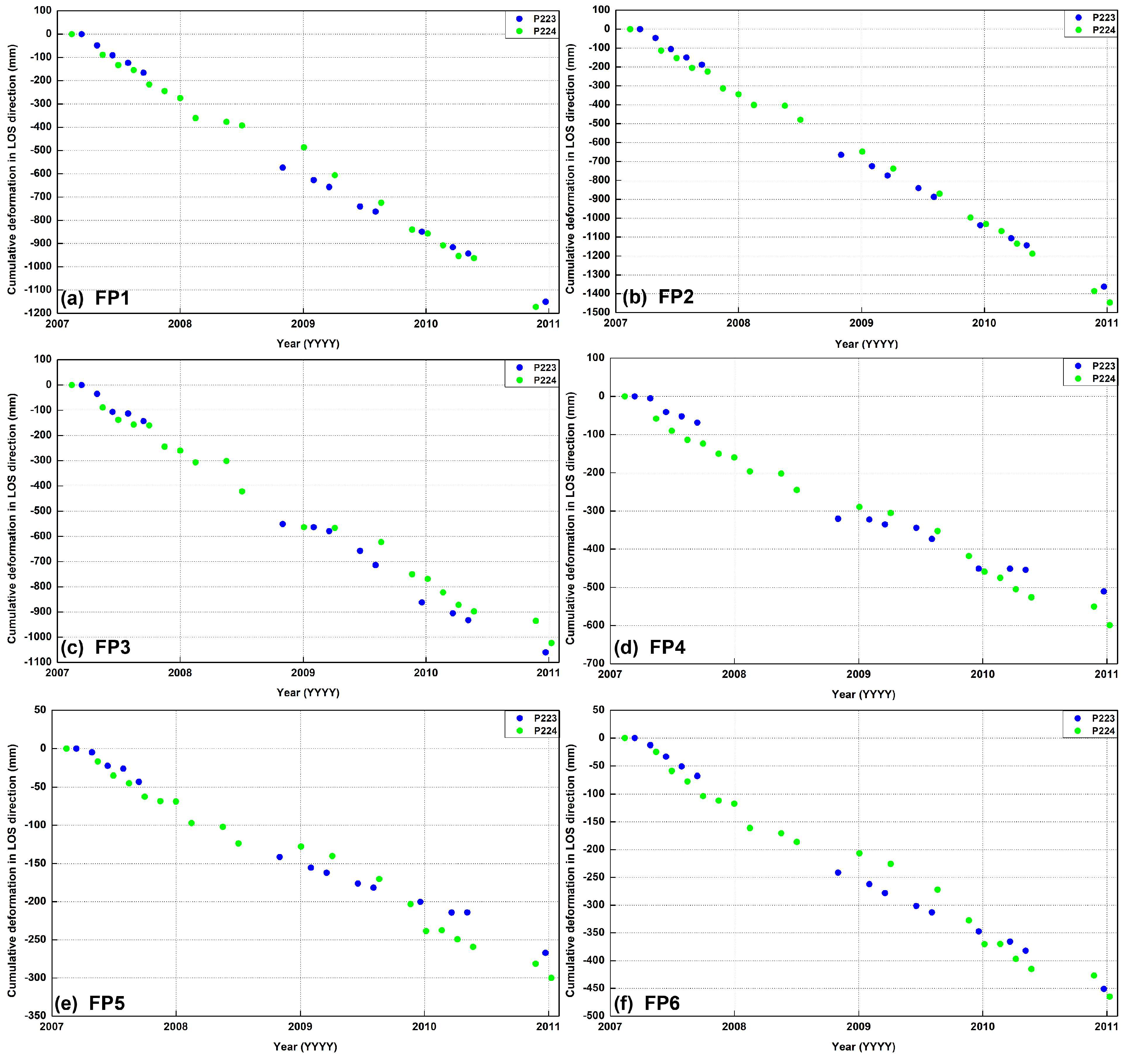
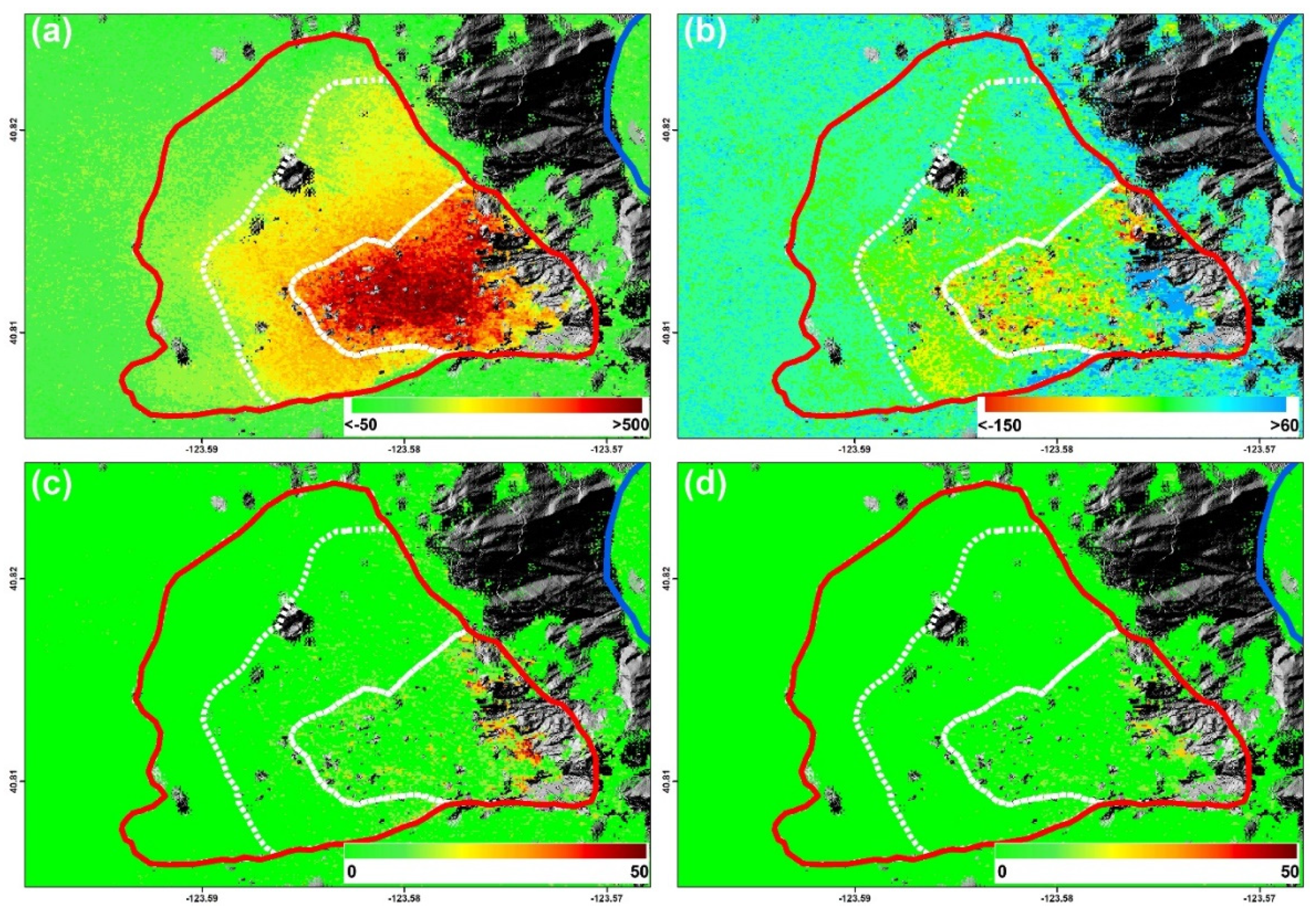
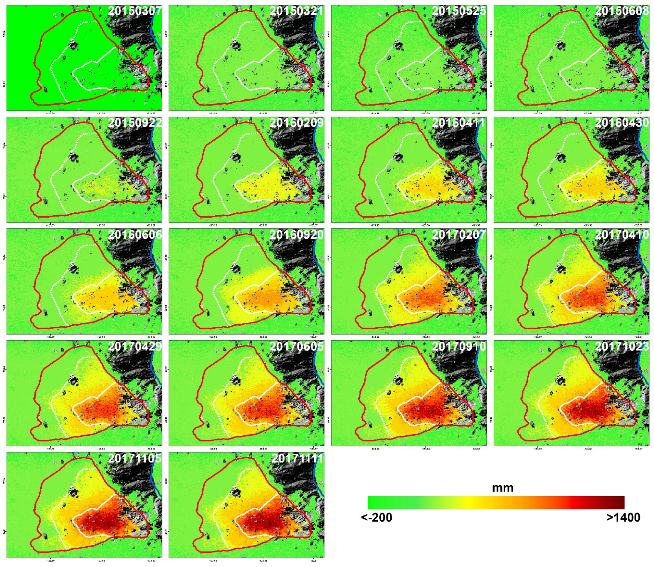
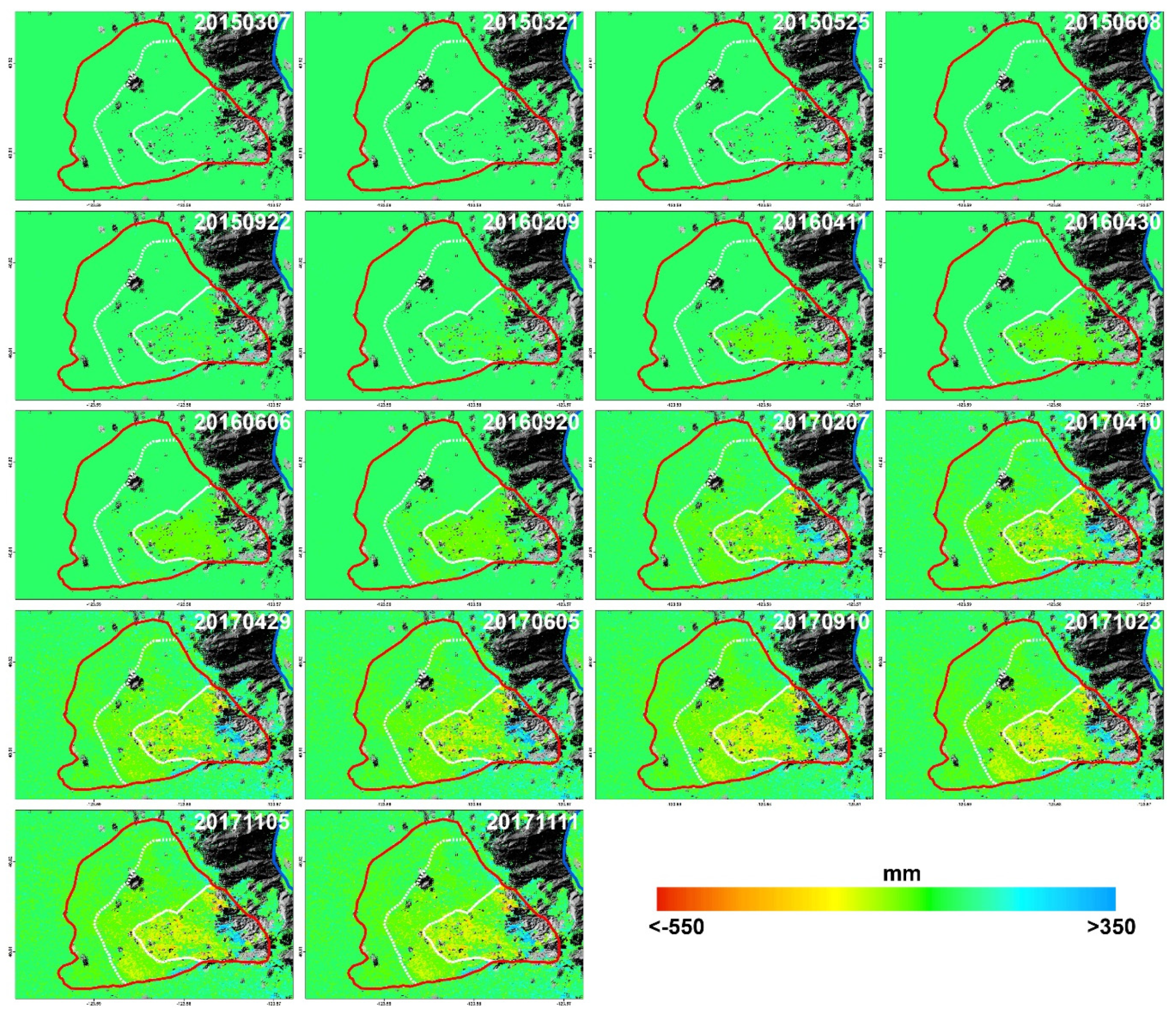
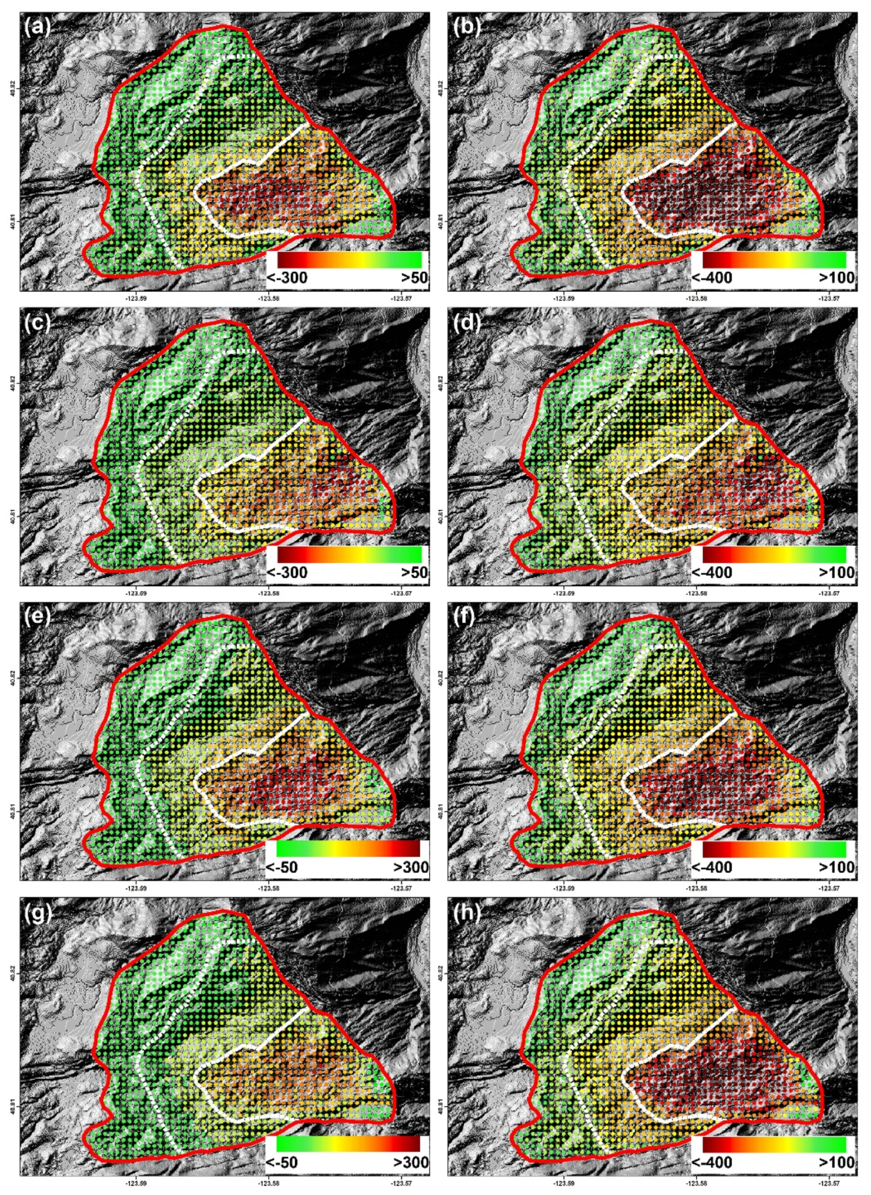
4.1. Line of Sight (LOS) Deformation Maps

The annual LOS deformation rates derived from each independent SAR datasets are shown in Figure 4a–f, respectively. It is worth noting that the positive values indicate the landslide motion toward the satellite sensor while the negative values represent the landslide motion away from the satellite sensor. As seen on the deformation maps, the large displacement mainly occurs in the eastern part of the Cedar Grove Ranch Earthflow, which is consistent with the active landslide identified by Zhao et al. [10]. The deformation distributions were similar, but the deformation magnitudes were slightly different for P223 and P224 during the period of 2007–2011 (Figure 4a,b). This is mainly because our study area is located in the near range of the P223 swath, but in the far range of the P224 swath, leading to a difference of around 2.7° between the two radar LOS directions for the same ground target. Furthermore, the average ascending LOS deformation rates were almost similar to those of the descending LOS velocities during the period of 2015–2017, but the signs were the opposite, indicating that the landslide moved toward the satellite sensor in the descending tracks, but away from the sensor in the ascending tracks (Figure 4c–f). These observations also suggest that the landslide displacements must be dominated by the horizontal motions. We can also see that the Three Bears landslide underwent strong movement with the deformation rate exceeding 300 mm/yr from 2007 to 2011, but the motions decreased to around 250 mm/yr from 2015 to 2017. The reasons can be summarized as follows: (1) It may be mainly caused by the sparse temporal sampling during the period of 2015–2017, especially for datasets P69 and P171; and (2) The study area suffered a persistent drought from the period of December 2011 to March 2017 [33], which may have also caused the reduction in the deformation rate.

To better analyze spatiotemporal characteristics of landslide motion, we focused on the time-series deformation from 2007 to 2011. Figure 5a,b show the time-series deformation of the active landslide along the radar LOS direction from two independent SAR datasets P223 and P224, respectively. The time-varying and spatial patterns were basically consistent. In general, the landslide moved slowly during the intervening summer months, but moved quickly in the wet seasons from November to April (Figure 6). Furthermore, we can also see in Figure 5a,b that ground movement was not spatially uniform within the active landslide region (red polygon), which can be segmented into three sections along its longitudinal axis: the zone of larger movement in the southeastern part of the landslide (Zone 1), the zone of medium movement in the middle part (Zone 2), and the zone of less movement in the northwestern part (Zone 3). The area of Zone 1 is about 0.79 km² with an average cumulative LOS deformation rate ranging from −200 mm/yr to −400 mm/yr, while the area of Zone 2 is around 0.95 km² with an average cumulative LOS deformation rate ranging from −60 mm/yr to −200 mm/yr from 2007 to 2011. The area of Zone 3 is about 0.85 km² with an average cumulative LOS deformation rate ranging from −10 mm/yr to −60 mm/yr from 2007 to 2011.

4.2. Two-Dimensional Deformation Estimation by Integrating Ascending and Descending ALOS PALSAR-2 Images

Combining the results shown in Figure 4c–f with the slope and aspect information derived from DEM data, it can be deduced that the Three Bears landslide primarily moved eastward horizontally. Since both ascending and descending ALOS PALSAR-2 data had the same time span from 2015 to 2017, we derived the east–west and vertical deformation components based on Equation (1) by using eight (six from P68 and two from P69) ascending interferograms and eighteen (fourteen from P170 and four from P171) descending interferograms.

The two-dimensional deformation rate maps and the corresponding standard deviations are shown in Figure 7. It can be seen that the east–west deformation rate varied from −50 mm/yr to 500 mm/yr (Figure 7a), while the vertical deformation rate ranged from −150 mm/yr to 50 mm/yr (Figure 7b), which only accounted for a third of the horizontal deformation. Furthermore, the east–west deformation pattern was very similar with the LOS time-series results shown in Figure 5, indicating that the landslide was dominated by eastward movement and relatively small vertical deformation. Moreover, the two-dimensional time-series deformations of the active landslide are presented in Figure 8 and Figure 9, respectively. It can be seen from Figure 8 that there was a continuous eastward movement of the landslide and obvious uneven deformation patterns were also visible during the whole monitoring period. The maximum cumulative east–west deformation from March 2015 to November 2017 could reach up to 1400 mm in Zone 1, but just 500 mm in Zone 2, and less than 300 mm in Zone 3. However, a different pattern and trend was seen in the cumulative vertical deformation. It can be seen from Figure 9: (1) that the landslide in Zone 1 experienced continuous subsiding deformation during the whole period with a maximum cumulative displacement up to −500 mm; (2) The landslide in Zone 2 presented a relatively small movement before February 2017 with an average deformation rate of −20.4 mm/yr, but moved quickly after February 2017 with an average deformation rate of −44.1 mm/yr, where the maximum vertical displacement amounted to −200 mm; and (3) The landslide in Zone 3 showed less vertical movement than the other two zones with a maximum vertical displacement just up to −100 mm during the period of March 2015 to November 2017.

5. Discussions

5.1. Verification of Deformation Results from Multi-Track Satellite Datasets

Since in situ observations were unavailable for our study area, we could not conduct the cross-validation with ground-truth data. Therefore, independent datasets with almost the same timespan were analyzed to verify the precision of the InSAR-derived results. In light of the different imaging geometries of SAR datasets, the radar LOS directions were different for the same ground target in each independent track, but the down-slope direction was identical by considering the amplification/scaling factor of different tracks based on Equation (2).

The slope angle and slope aspect $\beta$ and $\gamma$ can be derived based on the LS method if two or more different LOS observations can be obtained. To produce a stable solution, the deformation rates were down-sampled into 50 m. The optimal slope angle and slope aspect were finally determined by searching for the minimum residuals among the down-slope deformation rates from P68, P69, P170, and P171 in this study.

Figure 10 shows the LOS and down-slope deformation rates of the active landslide (red polygon in Figure 4), which were extracted separately from P68, P69, P170, and P171. The LOS deformation patterns from adjacent satellite tracks were similar to each other (e.g., P68 and P69, P170 and P171); but there were also differences in the magnitude of deformation rates, especially for the descending and ascending observations. However, the similar deformation values were clearly visible in the down-slope direction with the maximum down-slope deformation rate of about −450 mm/yr. Thus, we could draw the following conclusion: most of the difference in the LOS direction can be explained by the difference in the SAR looking angle between the adjacent satellite tracks. Meanwhile, the standard deviation of the down-slope difference between P68, P69, P170, and P171 was about 25.4 mm/yr. Accordingly, assuming the precisions of the results from independent paths were equal, the precision of the InSAR-derived measurement was around 18 mm/yr. The reason for this large discrepancy was mainly that there were only four usable short-duration interferograms involved in the deformation calculation for P69, which may have caused an underestimation in the deformation rate.

Due to the slight difference in the incidence angle between P223 and P224, the LOS deformation rates were compared to verify the precision of InSAR-derived results from 2007 to 2011. The corresponding standard deviation was about 23.4 mm/yr with the precision of 17 mm/yr.

5.2. Correlation between Landslide Motion and Seasonal Precipitation

A good correlation between the sliding acceleration and precipitation has been presented in many cases [34,35]. However, there is a time lag between the peaks of deformation and precipitation [10,34]. In order to reveal the correlation between landslide motion and precipitation, we collected historical rainfall data and compared it with the time-series deformation derived from ALOS PALSAR-1/2 satellites. An example at point FP2 (white cross shown in Figure 5a), which is located in Zone 1, is shown in Figure 11.

Singular value decomposition (SVD) [17] was first used to integrate the time-series deformation measurements from P223 and P224. The temporal intervals of integrated time-series deformation ranged from 17 to 184 days with an average of about 43 days. We can see that the results from these two independent tracks were consistent with each other (Figure 11a). The cumulative movement of −1530 mm along the LOS direction was projected as much as −2460 mm along the down-slope direction. Furthermore, the increased temporal sampling provides us with the possibility for us to better understand the landslide behavior in response to precipitation. Then, the linear trend component (black dash line in Figure 11a) was removed from the original InSAR-derived time-series result by using the linear regression model in order to reveal the seasonal kinemics of the landslide. Finally, to synchronize the temporal resolution of InSAR measurements and precipitation data, the linearly detrended down-slope displacements and 30-day accumulative precipitation were compared (Figure 11b). Since no meteorological station information could be directly obtained in the Three Bears landslide region, we obtained the daily precipitation records of the nearest rainfall monitoring gauge, which is 31.2 km east of the landslide, from the Department of Water Resources, California Data Exchange Center. As seen on the red bars of Figure 11b,d, the 30-day accumulative precipitation of the study area varied seasonally. The rainfall was abundant from October to April during the wet season (winter), which infiltrated and saturated the ground in the basal part of the landslide. Our results showed that sliding motion tended to accelerate almost immediately after the autumn rain began from October or November (gray box in Figure 11b). In particular, the landslide accelerated abruptly at the end of 2010 and the beginning of 2011 with a down-slope sliding rate of up to 10.5 mm/day between 23 December 2010 and 9 January 2011, which was about 10 times higher than the average rate per day during the whole monitoring period. This finding is consistent with the reconnaissance field investigation conducted by Forest Service Region 5 Northern Province geologists who observed that the landslide was very active during the winter of 2010–2011, and that the activity continued into the summer of 2011 [15].

A correlation analysis between the InSAR measurements and precipitation was also conducted for the period of 2015–2017 (Figure 11c,d). As expected, either linearly detrended east–west or vertical movements showed similar seasonal oscillations with the precipitation (Figure 11d). However, the response of the landslide motion to precipitation was not instantaneous, showing a certain time lag between the peaks of deformation and precipitation with a lag of about one month or more in our study. Similar phenomena have been reported elsewhere such as the Boulder Creek landslide in northern California with a lag of 1–2 months [10], and the Portuguese Bend landslide in southern California with a lag of 2–6 weeks [36]. Unfortunately, it is impossible to determine the time lag with better temporal resolution since the temporal sampling of ALOS PALSAR-2 data was low during the monitoring period.

6. Conclusions

Advanced InSAR time series methods are presented with multi-track L-band satellite SAR datasets to characterize the kinematics of the Three Bears landslide at the Cedar Grove Ranch covering two periods (2007–2011 and 2015–2017). First, one-dimensional (1-D) LOS deformation maps were generated individually from SAR datasets acquired by ascending ALOS PALSAR-1/2 and descending ALOS PALSAR-2 satellites. Then, cross-validation was carried out between the deformation results from independent tracks. The precision of the deformation rates derived from P223 and P224 (ALOS-1; 2007–2011) was 17 mm/yr in the LOS direction while the precision of the result from P68, P69, P170, and P171 (ALOS-2; 2015–2017) was 21 mm/yr in the down-slope direction. The east–west and vertical components of the landslide from 2015 to 2017 were retrieved by integrating the ascending and descending InSAR measurements, indicating that the landslide is dominated by eastward movement while the vertical deformation is relatively small, which suggests that it is a slow-moving landslide. Finally, the correlation between InSAR-derived measurements and seasonal precipitation revealed that greater deformation occurred following increased precipitation with a certain time lag.

It has been demonstrated that the movement of slow-moving landslides can be readily measured in the forested mountainous regions using advanced time-series InSAR analysis methods and L-band InSAR observations. This research provides first-hand, relatively complete, and accurate information about the Three Bears landslide. However, more detailed landslide motions cannot be revealed if based solely on ALOS PALSAR-1/2 datasets, due to the poor temporal resolutions. Airborne SAR missions (i.e., uninhabited aerial vehicle synthetic aperture radar (UAVSAR)), which can provide high spatial resolution images and various options for the imaging viewing geometries and acquisition time intervals, are highly promising to reveal the dynamics of landslide motions in a finer temporal scale.

The information on spatiotemporal deformation and general magnitude revealed by the methods applied by this investigation is extremely valuable in guiding risk assessments over broad areas as well as to focus further field investigations. These methods could also be used to identify precursory movements that may occur on other landslides prior to catastrophic failure [37]. Such investigations could focus on landslides that pose large adverse consequences to life and property.

References

1. Petley, D. Global patterns of loss of life from landslides. Geology 2012, 40, 927–930. [Google Scholar] [CrossRef]
2. Sidle, R.; Ochiai, H. Landslides: Processes, Prediction, and Land Use. Water Resources Monograph; American Geophysical Union: Washington, DC, USA, 2006. [Google Scholar]
3. Pinyol, N.M.; Alonso, E.E.; Corominas, J.; Moya, J. Canelles landslide: Modelling rapid drawdown and fast potential sliding. Landslides 2012, 9, 33–51. [Google Scholar] [CrossRef]
4. Uhlemann, S.; Smith, A.; Chambers, J.; Dixon, N.; Dijkstra, T.; Haslam, E.; Meldrum, P.; Merritt, A.; Gunn, D.; Mackay, J. Assessment of ground-based monitoring techniques applied to landslide investigations. Geomorphology 2016, 253, 438–451. [Google Scholar] [CrossRef]
5. Zhang, Y.; Tang, H.; Li, C.; Lu, G.; Cai, Y.; Zhang, J.; Tan, F. Design and Testing of a Flexible Inclinometer Probe for Model Tests of Landslide Deep Displacement Measurement. Sensors 2018, 18, 224. [Google Scholar] [CrossRef] [PubMed]
6. Calcaterra, S.; Cesi, C.; Di Maio, C.; Gambino, P.; Merli, K.; Vallario, M.; Vassallo, R. Surface displacements of two landslides evaluated by GPS and inclinometer systems: A case study in Southern Apennines, Italy. Nat. Hazards 2012, 61, 257–266. [Google Scholar] [CrossRef]
7. Casagli, N.; Frodella, W.; Morelli, S.; Tofani, V.; Ciampalini, A.; Intrieri, E.; Raspini, F.; Rossi, G.; Tanteri, L.; Lu, P. Spaceborne, UAV and ground-based remote sensing techniques for landslide mapping, monitoring and early warning. Geoenviron. Disasters 2017, 4, 9. [Google Scholar] [CrossRef]
8. Cignetti, M.; Manconi, A.; Manunta, M.; Giordan, D.; De Luca, C.; Allasia, P.; Ardizzone, F. Taking advantage of the ESA G-POD service to study ground deformation processes in high mountain areas: A Valle d’Aosta case study, northern Italy. Remote Sens. 2016, 8, 852. [Google Scholar] [CrossRef]
9. Solari, L.; Del Soldato, M.; Montalti, R.; Bianchini, S.; Raspini, F.; Thuegaz, P.; Bertolo, D.; Tofani, V.; Casagli, N. A Sentinel-1 based hot-spot analysis: Landslide mapping in north-western Italy. Int. J. Remote Sens. 2019, 40, 7898–7921. [Google Scholar] [CrossRef]
10. Zhao, C.Y.; Lu, Z.; Zhang, Q.; Fuente, J.D.L. Large-area landslide detection and monitoring with ALOS/PALSAR imagery data over Northern California and Southern Oregon, USA. Remote Sens. Environ. 2012, 124, 348–359. [Google Scholar] [CrossRef]
11. Hu, X.; Wang, T.; Pierson, T.C.; Lu, Z.; Kim, J.; Cecere, T.H. Detecting seasonal landslide movement within the Cascade landslide complex (Washington) using time-series SAR imagery. Remote. Sens. Environ. 2016, 187, 49–61. [Google Scholar] [CrossRef]
12. Kang, Y.; Zhao, C.Y.; Zhang, Q.; Lu, Z.; Li, B. Application of InSAR techniques to an analysis of the Guanling landslide. Remote Sens. 2017, 9, 1046. [Google Scholar] [CrossRef]
13. Zhao, C.Y.; Kang, Y.; Zhang, Q.; Lu, Z.; Li, B. Landslide identification and monitoring along the Jinsha River catchment (Wudongde reservoir area), China, using the InSAR method. Remote Sens. 2018, 10, 993. [Google Scholar] [CrossRef]
14. Kang, Y.; Lu, Z.; Zhao, C.Y.; Zhang, Q.; Kim, J.; Niu, Y.F. Diagnosis of Xinmo (China) landslide based on Interferometric Synthetic Aperture Radar observation and modeling. Remote Sens. 2019, 11, 1846. [Google Scholar] [CrossRef]
15. U.S. Department of Agriculture, Forest Service. Three Bears Landslide at Cedar Grove Ranch Lower South Fork Trinity River. Summary Report of a Reconnaissance Field Investigation; U.S. Department of Agriculture, Forest Service: Washington, DC, USA, 2014.
16. California Department of Water Resources, Northern District. South Fork Trinity Watershed Erosion Investigation; California Department of Water Resources, Northern District: Red Bluff, CA, USA, 1979; pp. 1–83.
17. Berardino, F.; Fornaro, G.; Lanari, R.; Sansosti, E. A new algorithm for surface deformation monitoring based on small baseline differential SAR interferometry. IEEE Trans. Geosci. Remote Sens. 2002, 40, 2375–2383. [Google Scholar] [CrossRef]
18. Werner, C.; Wegmuller, U.; Strozzi, T.; Wiesmann, A. Interferometric point target analysis for deformation mapping. In Proceedings of the International Geoscience and Remote Sensing Symposium, Toulouse, France, 21–25 July 2003; pp. 4362–4364. [Google Scholar]
19. Samsonov, S.V.; d’Oreye, N. Multidimensional small baseline subset (MSBAS) for two-dimensional deformation analysis: Case study Mexico City. Can. J. Remote Sens. 2017, 43, 318–329. [Google Scholar] [CrossRef]
20. Farr, T.G.; Rosen, P.A.; Caro, E.; Crippen, R.; Duren, R.; Hensley, S.; Kobrick, M.; Paller, M.; Rodriguez, E.; Roth, L.; et al. The shuttle radar topography mission. Rev. Geophys. 2007, 45, 33. [Google Scholar] [CrossRef]
21. Lu, Z.; Dzurisin, D. InSAR Imaging of Aleutian Volcanoes: Monitoring a Volcanic Arc from Space: Springer Praxis Books, Geophysical Sciences; Springer: Berlin/Heidelberg, Germany, 2014; 390p, ISBN 978-3-642-00347-9. [Google Scholar]
22. Handwerger, A.L.; Roering, J.J.; Schmidt, D.A.; Rempel, A.W. Kinematics of earthflows in the Northern California Coast Ranges using satellite interferometry. Geomorphology 2015, 246, 321–333. [Google Scholar] [CrossRef]
23. Wegmuller, U.; Walter, D.; Spreckels, V.; Werner, C.L. Nonuniform ground motion monitoring with TerraSAR-X persistent scatterer interferometry. IEEE Trans. Geosci. Remote Sens. 2010, 48, 895–904. [Google Scholar] [CrossRef]
24. Lanari, R.; Mora, O.; Mununta, M.; Mallorqui, J.; Berardino, P.; Sansonsti, E. A small baseline approach for investigating deformation on full resolution differential SAR interferograms. IEEE Trans. Geosci. Remote Sens. 2004, 42, 1377–1386. [Google Scholar] [CrossRef]
25. Sansosti, E.; Casu, F.; Manzo, M.; Lanari, R. Space borne radar interferometry techniques for the generation of deformation time series: An advanced tool for Earth’s surface displacement analysis. Geophys. Res. Lett. 2010, 37, L20305. [Google Scholar] [CrossRef]
26. Lee, C.W.; Lu, Z.; Jung, H.S.; Won, J.S.; Dzurisin, D. Surface deformation of Augustine Volcano (Alaska), 1992–2005, from multiple-interferogram processing using a refined SBAS InSAR approach. In The 2006 eruption of Augustine Volcano, Alaska: U.S. Geological Survey Professional Paper 1769; Power, J.A., Coombs, M.L., Freymueller, J.T., Eds.; U.S. Geological Survey: Reston, VA, USA, 2010; Chapter 18; pp. 453–465. Available online: http://pubs.usgs.gov/pp/1769/chapters/p1769_chapter18.pdf (accessed on 4 November 2019).
27. Chen, C.W.; Zebker, H.A. Two-dimensional phase unwrapping with the use of statistical models for cost functions in nonlinear optimization. J. Opt. Soc. Am. A 2001, 18, 338–351. [Google Scholar] [CrossRef] [PubMed]
28. Wright, T.J.; Parsons, B.E.; Lu, Z. Toward mapping surface deformation in three dimensions using InSAR. Geophys. Res. Lett. 2004, 31. [Google Scholar] [CrossRef]
29. Hu, J.; Li, Z.W.; Ding, X.L.; Zhu, J.J.; Zhang, L.; Sun, Q. Resolving three-dimensional surface displacements from InSAR measurements: A review. Earth-Sci. Rev. 2014, 133, 1–17. [Google Scholar] [CrossRef]
30. Samsonov, S.; d’Oreye, N. Multidimensional time-series analysis of ground deformation from multiple InSAR data sets applied to Virunga Volcanic Province. Geophys. J. Int. 2012, 191, 1095–1108. [Google Scholar]
31. Hu, X.; Lu, Z.; Pierson, T.C.; Kramer, R.; George, D.L. Combining InSAR and GPS to Determine Transient Movement and Thickness of a Seasonally Active Low-Gradient Translational Landslide. Geophys. Res. Lett. 2018, 45, 1453–1462. [Google Scholar] [CrossRef]
32. Hilley, G.E.; Bürgmann, R.; Ferretti, A.; Novali, F.; Rocca, F. Dynamics of slow-moving landslides from permanent scatterer analysis. Science 2004, 304, 1952–1955. [Google Scholar] [CrossRef] [PubMed]
33. Drought in California. Available online: https://www.drought.gov/drought/states/california (accessed on 4 November 2019).
34. Raspini, F.; Bianchini, S.; Ciampalini, A.; Del Soldato, M.; Montalti, R.; Solari, L.; Tofani, V.; Casagli, N. Persistent Scatterers continuous streaming for landslide monitoring and mapping: The case of the Tuscany region (Italy). Landslides 2019, 16, 2033–2044. [Google Scholar] [CrossRef]
35. Rosi, A.; Lagomarsino, D.; Rossi, G.; Segoni, S.; Battistini, A.; Casagli, N. Updating EWS rainfall thresholds for the triggering of landslides. Nat. Hazards 2015, 78, 297–308. [Google Scholar] [CrossRef]
36. Calabro, M.D.; Schmidt, D.A.; Roering, J.J. An examination of seasonal deformation at the Portuguese Bend landslide, southern California, using radar interferometry. J. Geophys. Res. Earth Surf. 2010, 115. [Google Scholar] [CrossRef]
37. Stevens, M. Analyzing the Preliminary Movement of the East Branch of East Weaver Creek Landslide Prior to the Catastrophic Failure in Spring 2011 as Detected by InSAR. Master’s Thesis, Humboldt State University, Arcata, CA, USA, 2014. [Google Scholar]
Figure 1. Study area and coverage of the SAR datasets. (a) Spatial coverage of ALOS PALSAR-1/2 satellite datasets (white boxes) superimposed on the shaded relief map. The red star represents the study area, while the blue lines represent the main rivers in the study area. The inset map presents the location of the study area in northern California, USA. (b) Enlarged shaded relief map of the Three Bears landslide generated by 1-m resolution LiDAR DEM. The blue lines show creeks and streams, and the thick blue line represents the South Fork Trinity River (SFTR). The brown polygon shows the dormant landslides identified by the United States Forest Service (USFS) while the polygon outlined in black indicates the boundary of the Cedar Grove Ranch Earthflow. The active landslide identified by Zhao et al. [10] is highlighted by a thick red polygon. (c) A field photo of the landscape around the Three Bears landslide (view northwest), provided by Juan de la Fuente.
Remotesensing 11 02726 g001
Figure 2. Temporal-spatial baseline distribution of selected interferograms used in this study. The SAR acquisition dates are shown in the format of YYYYMMDD (e.g., 20070314) while Y-axis represents the perpendicular baseline of the interferogram. (a) and (b) show the interferograms generated by ascending ALOS PALSAR-1 data for Path 223 (P223) and Path 224 (P224); (c) and (d) show the interferograms generated by ascending ALOS PALSAR-2 data for Path 68 (P68) and Path 69 (P69); (e) and (f) show the interferograms generated by descending ALOS PALSAR-2 data for Path 170 (P170) and Path 171 (P171).
Remotesensing 11 02726 g002
Figure 3. An example of unwrapping error correction based on a deformation model. (a) The original unwrapped phase of a 364-day interferogram (e.g., 20150922–20160920 for P68). (b) The corresponding deformation model constructed from a stack of correctly-unwrapped short-duration interferograms. (c) The new unwrapped phase with the aid of deformation model. (d) and (e) show the unwrapped phase extracted along the profile P1P1′ and P2P2′, respectively. The red polygon shows the boundary of the active landslide and the white lines represent the location of the profiles.
Remotesensing 11 02726 g003
Figure 4. Average LOS deformation rate maps of the Three Bears landslide calculated with L-band SAR datasets (unit: mm/yr). The figures in the first and second row show the results derived from ascending datasets: (a) P223 of ALOS PALSAR-1 (data period: 2007–2011), (b) P224 of ALOS PALSAR-1 (data period: 2007–2011), (c) P68 of ALOS PALSAR-2 (data period: 2015–2017), and (d) P69 of ALOS PALSAR-2 (data period: 2014–2017). The figures in the third row show the results derived from descending datasets: (e) P170 of ALOS PALSAR-2 (data period: 2015–2017) and (f) P171 of ALOS PALSAR-2 (data period: 2015–2017).
Remotesensing 11 02726 g004
Figure 5. Cumulative deformation along the radar LOS direction for (a) Path 223 (P223) from 14 March 2007 to 23 December 2010 with the reference SAR acquisition date 20070314 and (b) Path 224 (P224) from 13 February 2007 to 9 January 2011 with the reference SAR acquisition date 20070213. The color scale shows the LOS deformation in millimeters and the white line represents the boundary of different sections inferred by the InSAR-derived deformation pattern and the compressional morphologic features. It is worth noting that the positive values indicate the landslide motion toward the satellite sensor, while the negative values represent the landslide motion away from the satellite sensor.
Remotesensing 11 02726 g005
Figure 6. Cumulative deformation along the radar LOS direction for Path 223 (blue dots) and Path 224 (green dots) of six feature points (FP1, FP2, FP3, FP4, FP5, and FP6) as shown in Figure 5a.
Remotesensing 11 02726 g006
Figure 7. Two-dimensional deformation rate maps from 2015 to 2017 calculated from ascending and descending SAR datasets (unit: mm/yr): (a) the east–west deformation; (b) the vertical deformation; (c) the standard deviation (STD) of the estimated east–west deformation rate; and (d) the standard deviation (STD) of the estimated vertical deformation rate. The red polygon shows the active landslide, while the white line represents the boundary of different sections inferred by the InSAR-derived deformation pattern and the compressional morphologic features.
Remotesensing 11 02726 g007
Figure 8. Cumulative east–west deformation from 7 March 2015 to 11 November 2017 inverted by using ascending and descending ALOS PALSAR-2 satellite datasets. It is worth noting that the positive values indicate eastward movement while the negative values represent westward movement.
Remotesensing 11 02726 g008
Figure 9. Cumulative vertical deformation from 7 March 2015 to 11 November 2017 inverted by using ascending and descending ALOS PALSAR-2 satellite datasets.
Remotesensing 11 02726 g009
Figure 10. Average annual LOS (left column) and down-slope (right column) deformation rates of active landslide extracted from P68 ((a) and (b)), P69 ((c) and (d)), P170 ((e) and (f)) and P171 ((g) and (h)) (unit: mm/yr). It is worth noting that the same color legend is used in the right column but a different one in the left column.
Remotesensing 11 02726 g010
Figure 11. Correlation between the InSAR-derived time-series measurements and 30-day accumulative precipitation. (a) Cumulative down-slope movement at FP2 (shown in Figure 5a) by fusing time-series deformation from P223 (blue dots) and P224 (green dots) with the singular value decomposition (SVD) method (2007–2011). (b) Comparison between linearly detrended down-slope movement and 30-day accumulative precipitation records. (c) Cumulative east–west and vertical movement at FP2 by fusing the ascending and descending interferograms (2015–2017). (d) Comparison between linearly detrended two-dimensional movement and 30-day accumulative precipitation records. Here, the point targets within 50 m × 50 m window, centered on the point FP2, were involved to compute the corresponding uncertainty of the time-series deformation. The error bar represents one sigma. The gray box shown in (b) and (d) indicates the sliding acceleration timespan. The pink pentagram shown in (b) indicates the time of the 6.5 Mw earthquake on 9 January 2010.
Remotesensing 11 02726 g011