Distinguishing Photosynthetic and Non-Photosynthetic Vegetation: How Do Traditional Observations and Spectral Classification Compare?

Abstract

Remotely sensed ground cover maps are routinely validated using field data collected by observers who classify ground cover into defined categories such as photosynthetic vegetation (PV), non-photosynthetic vegetation (NPV), bare soil (BS), and rock. There is an element of subjectivity to the classification of PV and NPV, and classifications may differ between observers. An alternative is to estimate ground cover based on in situ hyperspectral reflectance measurements (HRM). This study examines observer consistency when classifying vegetation samples of wheat (Triticum aestivum var. Gladius) covering the full range of photosynthetic activity, from completely senesced (0% PV) to completely green (100% PV), as photosynthetic or non-photosynthetic. We also examine how the classification of spectra of the same vegetation samples compares to the observer results. We collected HRM and photographs, over two months, to capture the transition of wheat leaves from 100% PV to 100% NPV. To simulate typical field methodology, observers viewed the photographs and classified each leaf as either PV or NPV, while spectral unmixing was used to decompose the HRM of the leaves into proportions of PV and NPV. The results showed that when a leaf was ≤25% or ≥75% PV observers tended to agree, and assign the leaf to the expected category. However, as leaves transitioned from PV to NPV (i.e., PV ≥ 25% but ≤ 75%) observers’ decisions differed more widely and their classifications showed little agreement with the spectral proportions of PV and NPV. This has significant implications for the reliability of data collected using binary methods in areas containing a significant proportion of vegetation in this intermediate range such as the over/underestimation of PV and NPV vegetation and how reliably this data can then be used to validate remotely sensed products.

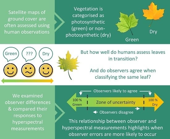
1. Introduction

Remotely sensed fractional cover maps are critically important for understanding a variety of environmental issues such as the impacts of land use change, climate change variability, ecosystem function, and desertification [1,2]. Algorithms used to produce fractional cover maps decompose each pixel in an image into a measure of similarity to two or more spectrally distinct land cover types, typically including photosynthetic vegetation (PV), non-photosynthetic vegetation (NPV), bare soil (BS), shadow, and snow [3,4]. This results in quantitative estimates of the fraction or proportion of the cover types that comprise image pixels.

During the production of these fractional cover maps some form of reference data is required for calibration and validation, typically derived from on-ground measurements. Commonly-used field methods for estimating fractional ground cover require observers to walk across a study area and make point-based observations at defined intervals. These methods use variants of point-based sampling techniques that were initially developed for vegetation ecology and rangeland assessment [5,6,7]. They can also be used for more detailed surveys such as determining the presence or abundance of plant species across a survey area [8,9].

When estimating fractional cover within a defined sampling area observers typically make hundreds of point-based assessments which are collated to produce overall estimates of fractional cover for each cover type across the site. Some cover types are discrete, well defined classes (e.g., “rock”, “cryptogam”, or “litter”) that are easily discriminated with high accuracy. However, PV and NPV are more accurately thought of as the extremes of a continuum, rather than binary categories, and therefore, distinguishing between PV and NPV can be a difficult task for observers. Moreover, there is little information on how consistently different observers categorise samples across the PV/NPV continuum.

This uncertainty is widely acknowledged and dealt with to some degree in standard field methods. For instance, Muir et al. [10] technical handbook outlines a simple, systematic and repeatable method to ensure the collection of consistent observations of fractional ground cover. This method has been implemented in Australia across a national network of ground cover sites and is used to calibrate and validate a variety of remotely sensed fractional cover datasets including the Commonwealth Scientific and Industrial Research Organisation (CSIRO) fractional cover product [11] and the Joint Remote Sensing Research Program (JRSRP) Landsat fraction cover product [12]. Muir’s method surveys 100 m transects and was designed initially to validate Landsat products allowing the average fractional cover values from a cluster of Landsat pixels (90 m²) to be compared to in situ fractions. When this field method is used to validate the CSIRO product, which has a spatial resolution of 500 m, it requires the field observations to be up-scaled. In order for these sites to be up-scaled the area surrounding the site needs to fit a specific criteria; (1) the species composition and cover should be spatially consistent and (2) that minimal topographic variation should occur across the site and surrounding area [10,13].

Field measurements for validating satellite-derived land cover products come with a number of limitations. Firstly, the data is often thought of as ‘ground truth’, but because of the sampling techniques involved, there is the potential to introduce errors. Secondly, acquiring calibration and validation data is often time-consuming and costly due to the number of sites required, the labor needed and distance required to travel to sites that may be dispersed across large areas. Thirdly, human subjectivity is known to be a significant contributing factor in the variability of vegetation field estimates, particularly when identifying NPV.

A potential solution to help reduce human error is to estimate the relative fractions of PV, NPV, and BS from field-based hyperspectral reflectance measurements. This method allows for many spectra to be recorded over a defined area, which capture the combined spectral response of the site in their aggregate. These spectra can then be unmixed to estimate the relative fractions of PV, NPV, and BS. Using this approach Meyer and Okin [14] demonstrated stronger agreement between fractional cover derived from field-based reflectance measurements and remotely sensed imagery than between traditional line-point intercept observations and remotely sensed imagery. However, as there was no ultimate point of truth for field cover, it was not possible to tell which measurements best represented reality. Thus, the collection of field spectral reflectance is a potential alternative to observer surveys, but we have a limited understanding of how this data compares when categorising PV and NPV. We are especially uncertain how spectral fractional cover estimates compare to human assessments as vegetation transitions from photosynthetic (green) to non-photosynthetic (dry). For the purpose of this study the spectral samples were considered a less subjective method of classifying vegetation and therefore used as a point of truth for the comparisons though acknowledge that there still remains uncertainties in the spectral measurements.

The overall aim of this study was to examine how human assessments compare to spectral fractional cover estimates, with a particular focus on how humans categorise vegetation across the PV/NPV continuum. Specifically, the research compared how vegetation is classified as photosynthetic and non-photosynthetic through observer surveys, replicating decisions made during field surveys, versus spectral unmixing of hyperspectral vegetation spectra. The key objectives were to understand when observers categorise vegetation as green or dry, determine the amount of variation between observers (if any) and to analyse how spectral classification compares to observation-based classification of vegetation.

2. Materials and Methods

2.1. Wheat Plants

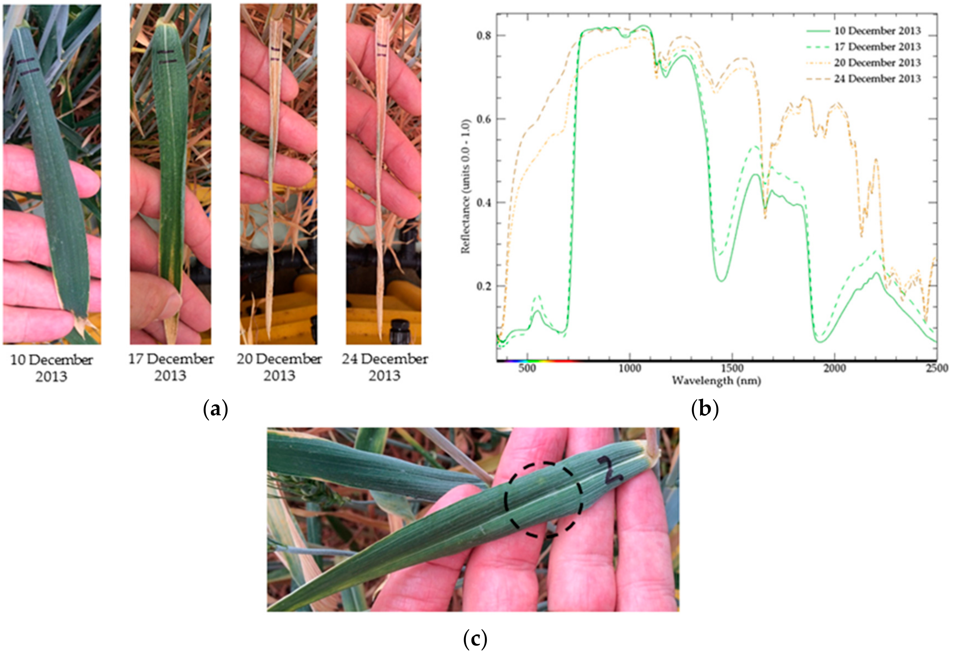
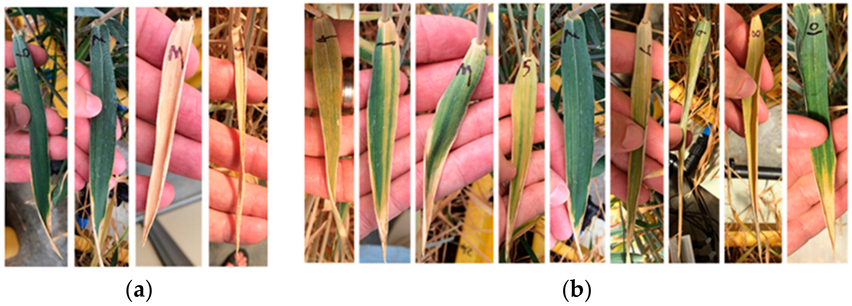
Wheat plants (Triticum aestivum var. Gladius) sown during August 2013 were grown in pots and monitored throughout their development in a glasshouse at the South Australian Research and Development Institute Plant Research Centre, University of Adelaide. Once the wheat reached maturity, single leaves from 12 separate plants were selected and labelled. To capture plant transition from maturity through to the end of senescence each of the 12 leaves was sampled over a two month period. During this period, the 12 leaves were photographed to create a visual record (Figure 1a), and hyperspectral measurements of reflectance (Figure 1b) were taken using an ASD Inc. (Analytical Spectral Devices) FieldSpec 3 spectroradiometer. This instrument measures the visible to shortwave infrared (350–2500 nm) parts of the electromagnetic spectrum in 2150 bands with a spectral sampling interval of 3 nm for 350–1000 nm and 10 nm for 1000–2500 nm. Leaf spectra were recorded with an ASD leaf-clip, an accessory specifically designed for recording leaf spectra under controlled lighting and geometry. Measurements were taken from the same part of each leaf, approximately 3 cm from the base of the leaf, on each sample date (Figure 1c).

2.2. Observer-Based Binary Classification

A questionnaire was developed to simulate observer field classifications of vegetation samples as either a green leaf (PV) or dry leaf (NPV) when using the Muir et al. [10] technique and definitions. From the photographs taken over a two month period, 74 were randomised and developed into the survey, with the leaves chosen to ensure a mix of different stages of senescence. Thirty-two observers were asked to perform a binary classification of each leaf as either green or dry. The observers consisted of university staff and students ranging from experienced field observers with a background in remote sensing and ecology to staff and students with no experience in the field or in remote sensing. Prior to the survey, all observers read the Muir et al. [10] definitions of a green leaf and a dry leaf (

Table 1. Definition of a green and dry leaf according to Muir et al. [10].

Category	Definition
Green Leaf	A leaf with green pigmentation (one that is actively photosynthesising) attached to a plant. Leaves may appear more yellow than green.
Dry Leaf	A leaf with non‑green pigmentation (one that is not actively photosynthesising). Includes senescing (but still living vegetation) and dead vegetation. Leaf must be attached to a plant or the ground.

) and subsequently classified the 74 leaves in a closed format survey based on their interpretation of the definitions provided. The classifications were based on observations of the small area of leaves where the spectral samples were taken (Figure 1c) and each leaf was viewed individually and classified before moving on to the next leaf.

2.3. Spectral Unmixing

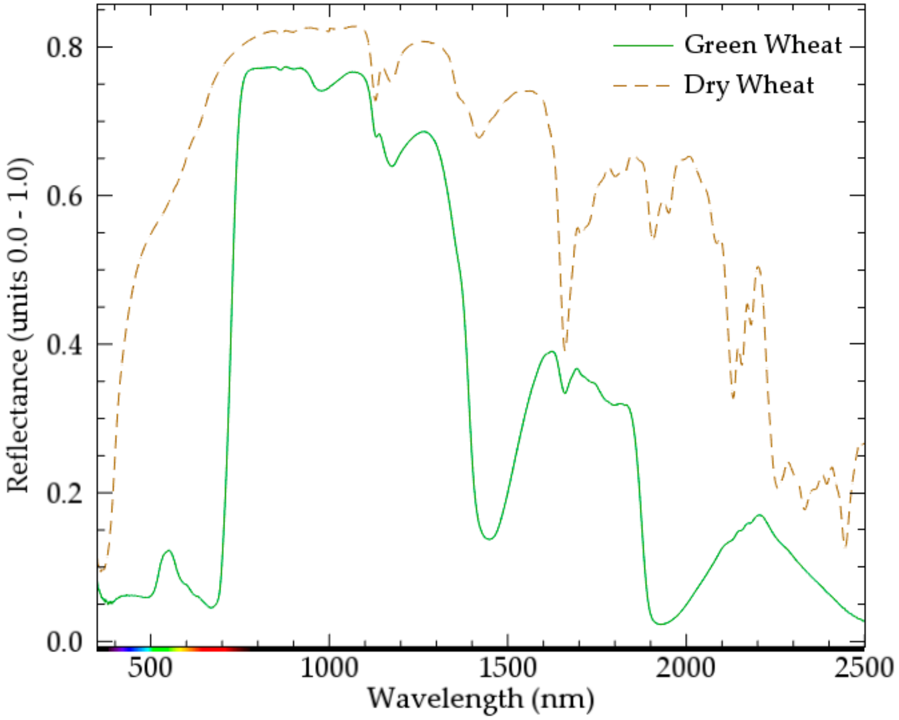
Photosynthetic and non-photosynthetic fractions of the 74 leaf spectral samples were derived by spectral unmixing. Reference spectra (endmembers) for the unmixing were selected from leaves not included in the survey (Figure 2).

The individual leaf spectra were converted into a single raster-like file which was processed using the linear spectral unmixing tool in ENVI 5.3.1 (Exelis Visual Information Solutions, Boulder, Colorado) and the reference spectra were used to decompose each of the spectral samples into relative proportions of green and dry. The partially constrained linear spectral unmixing algorithm [15,16,17] used was:

$$D{N}_b= {\sum }_{i=1}^n{F}_{e}D{N}_{e,b}+ E_{b } \mathrm{and} {\sum }_{i=1}^n{F}_e=1 ,$$

(1)

where $D{N}_b$ is the apparent surface reflectance of a pixel in band b of an image; $F_e$ is the fraction of endmember $e$; $D{N}_{e,b}$ is the relative reflectance of endmember $e$ in band b; $n$ is the number of endmembers, and $E_b$ is the error for band b of the fit of $n$ spectral endmembers. The unmixing resulted in three values for each leaf; the PV fraction, NPV fraction, and the root mean squared error (RMSE). Overall, the RMSE for each leaf showed very low errors with the highest RMSE reported as 0.08%. This provides confidence in the fractions of PV and NPV derived from the unmixing. Past studies show that PV can be predicted with high accuracy from spectral unmixing while typically NPV is harder to estimate [18,19]. The reflectance measurements were taken in a way to ensure no other materials such as soil or litter would be recorded by the sensor which can cause confusion during unmixing. Considering these factors, we can have a high degree of confidence in the spectral unmixing. In this paper PV and NPV is used to refer to the spectral classification of the leaves while ‘green’ and ‘dry’ refers the observer classifications. PV/ green leaf are equivalent categories, as are NPV/ dry leaf.

2.4. Statisical Analysis

To summarise the individual green and dry observations, descriptive statistics were used to calculate the total number of green observations and dry observations as a percentage of the total number of leaves (n = 74). Based on these totals, the grouped mean was calculated for both green and dry classes along with the standard deviation. These summary statistics were repeated for the spectral measurements of each leaf, calculating the average PV and NPV percentage based on the PV and NPV fractions derived for each leaf from the linear unmixing.

To test the relationship between the PV fractions and the green observations the raw individual observations and spectral unmixing fractions were analysed. Logistic regression was used to model the binary observer response variable (i.e., green or not green). PV was the single, linear, fixed-effects predictor in the model, and observer identity was fitted as a random intercept effect to account for the repeated measures by observers in scoring all photographs. The regression was calculated in R using a generalized linear mixed-effect model (GLMM) [20]. A detailed explanation of the GLMM can be found in Chambers, et al. [21]. Using the GLMM output parameters the confidence intervals (CI) were calculated.

3. Results

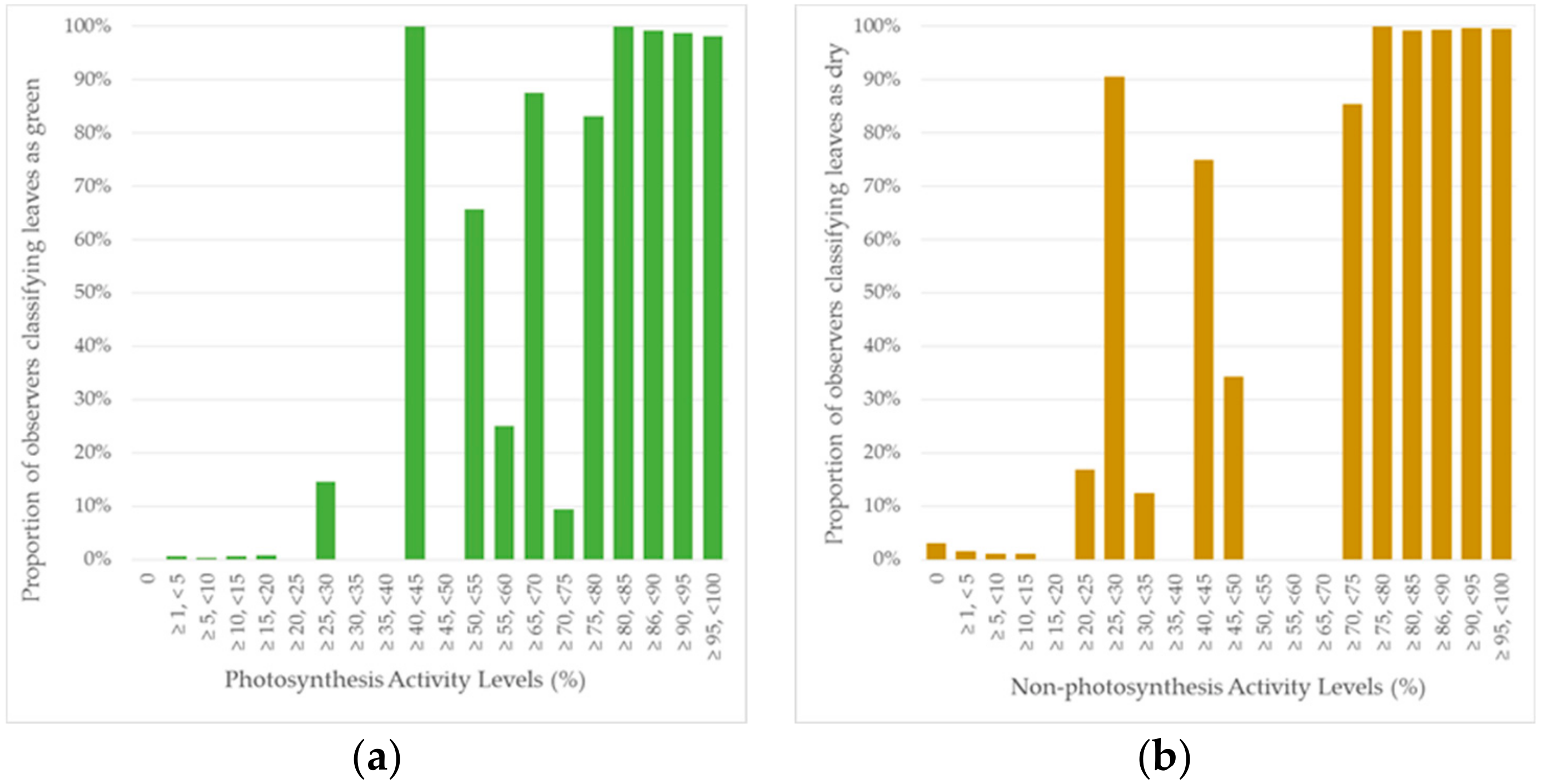
Firstly, we explored the observers’ classifications to determine their variation within the green and dry categories. Individual observers categorised 32–49% of the leaves in our sample as green and 51–65% as dry. The majority (73%) of observer responses were situated within the 91–100% range representing 54 of the 74 leaves analysed (Figure 3). These 54 leaves (Figure 4a) were unanimously classified as either a green or dry leaf by the observers. Of the remaining 20 leaves, 11 showed 90–99% agreement between the observers, while the remaining 9 leaves (Figure 4b) had the most substantial variation in observer responses.

The grouped mean proportions of green and dry leaves within the sample were 42% green and 58% dry, with a standard deviation of 3.82% for both green and dry showing that overall there is little variation amongst the observers. The average fractions of PV and NPV were 44.68% and 55.31%. The green and dry observational data, and PV and NPV fractions are both inverse of each other. From here on we will report only the green and PV results.

The GLMM likelihood ratio test between the spectral and observer results showed a strong positive linear relationship between the PV fractions and green observations (χ² = 2358.2, df = 1, p < 0.001). The GLMM also provided a value for the odds of an observer classifying a leaf as green. In this case, the odds of an observer scoring green increased by 10% with every one percent increase in the PV fraction (95% CI = 9.3%, 10.9%). It is important to note that this increase is relative to each observer. For example, some observers classify leaves as green, on average, at lower PV values, thereby reaching 100% PV more slowly, while others classify a leaf as green much later in the continuum and will reach 100% very quickly.

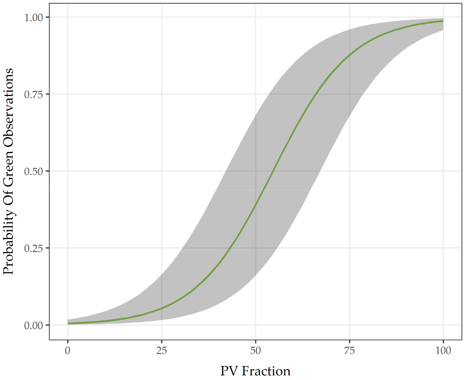
Based on the GLMM, the predicted mean observer values were calculated and represented as a line of best fit along with its confidence intervals (Figure 5). This confirms that at the extremes, when a leaf is extremely dry (0–(~25%)) or extremely green (PV ~75–100%) as classified by spectral unmixing, observers were almost all in agreement, and made the most appropriate classification. In the middle of the PV/NPV continuum (between ~25% and ~75% green) there is a zone of uncertainty where we saw observer decisions considerably differed from one another.

4. Discussion

The aim of this study was to investigate how human assessments compare to spectral estimates of fractional cover. By having multiple observers assess the same samples, we have developed an insight into the consistency of observer classifications and have also clarified the relationship between human and spectral assessments of PV and NPV.

When assessing the variation in the human observation of green and dry classes, there was a 17% difference between the minimum and maximum green proportions and a 14% difference between the dry proportions. Comparison of variation between observer results is not something that can be done routinely in the field because, typically, a single person would survey a specific area or transect due to time and cost. One study that examined the variability of fractional ground cover reference data between experienced and inexperienced observers found that there was no significant difference between mean estimates of cover based on experience level [22]. They noted that variation did increase between experienced and inexperienced observers for PV and NPV and that, for all observers NPV was the hardest to identify. It is important to note this variation when comparing these observed estimates to PV and NPV from satellite-derived fractional cover maps. While this variation is small, it is important to recognise when designing field methods and may influence cover estimates when multiple observers are contributing to one larger dataset.

Unanimous agreement between observers does not necessarily mean that the observers were correct but does suggest strong agreement among the observers for those specific leaves. When observers perform these classifications, they are required to make binary decisions, and in order to gain consistent data, it is vital that all observers have the same understanding of the definitions they are using. After our survey, observers provided feedback on the definitions (Table 1) upon which they based their decisions. A comment expressed by many was that the green and dry leaf definitions were not clear and that they appeared contradictory. When using these definitions it can be difficult for observers to define the point at which they should classify a leaf as green or dry and for this decision to be consistent between a group of observers. If an observer chooses to honour the dry leaf definition, anything with non-green pigmentation should be considered dry, meaning that an observer potentially would only classify a leaf as green if it was entirely green even though the green leaf definition stated that it could be more yellow than green. Another potential confounding factor is that a leaf may still be photosynthesising even if it has patches of yellow or appears dry, which was observed in a small number of leaves in the survey. An area of future research would be to improve these definitions clarifying how to classify any leaf into the green/dry categories.

There was a strong positive linear relationship between observer decisions and the spectral classification of each leaf. A limitation of this study is that the majority of the leaves fell within the top and bottom 25% of the photosynthetic continuum with few leaves spread across the mid 50% range: This distribution is likely to have influenced the results of the GLMM. When leaves were close to being completely green or dry, both the observers and spectral unmixing results were strongly related, but as the leaf transitioned this relationship became unclear. This is consistent with past studies that extract PV from in remotely sensed imagery using spectral unmixing techniques finding that PV can be reliably extracted [22,23]. The classification of leaves by observers within this 50% range can occur as follows; (1) a leaf that is classified as ~25% PV might be assessed as green by 0%, 5%, or 35% of observers, (2) a leaf that is ~55% PV might be assessed as green by 30% or 100% of observers and (3) a leaf that is ~70% PV might be assess as green by 0%, 20%, or 85% of human observers. Therefore, human classification of leaves with a mixture of PV and NPV (i.e., within the mid 50% of the spectral range) shows little agreement with the spectral proportions of PV and NPV. To examine these results further, a survey including more leaves within the mid-range of the PV/ NPV continuum would be desirable and is a potential area for future research. The GLMM also tested the odds of the relationship between the observer and spectral results and showed that the odds of an observer classifying a leaf as green increases by 10% for every 1% increase in the PV fraction relative to the observer’s last decision.

The use of wheat (Triticum aestivum var. Gladius) was an ideal choice to visually capture the transition of leaves from green to dry. Growing wheat in a controlled environment ensured that photographs and reflectance measurements of the same leaves could be taken over time with the results providing a baseline understanding of how observers can react when categorizing vegetation. No work was performed to test if these results could be generalized across other plant species but our results should be generalizable across other spectrally similar C3 plants as well as other green plants that lack any other significant source of pigmentation.

Spectral sampling provided a continuous and objective means to collect the reflectance of vegetation for spectral unmixing. The linear spectral unmixing results showed that very few leaves were entirely classified as PV or NPV and highlights the benefit of a survey method that can record continuous, rather than binary data. The ability to measure and analyse reflectance of vegetation or ground cover is a key advantage of this technique as it removes the need for observers to make binary decisions in the field. A recommendation for future studies is that if all vegetation is expected to be <75% PV or NPV either spectral sampling or observer surveys are appropriate. If the majority of the vegetation is situated between ~25% and ~75% PV, observer surveys are likely to introduce uncertainty and therefore we recommend spectral sampling. Spectral sampling enables the collection of more quantitative information to be collected over a study area and may allow for a more accurate assessment of relative PV or NPV status of vegetation to be attained for the purpose of training and evaluating earth observation products.

5. Conclusions

The collection of field-based calibration and validation data is critical for ensuring the accuracy and consistency of remotely sensed fractional ground cover products. This study provides a greater understanding of the variation that may occur between observer decisions and when this data may become less reliable. In addition, it clarifies the relationship between human and spectral assessment of PV and NPV, highlighted by the follow key findings. Firstly, when comparing the proportions of PV and NPV between observers, there was up to 17% variation between observers for PV and up to 14% variation for NPV. This variation can have implications for the consistency of data collected using multiple observers and how accurately satellite-derived ground cover products can be calibrated and validated using this data. Secondly, the GLMM suggests that the PV and NPV values for the observer and spectral data were similar but shows that observers overestimated NPV and underestimated PV. Lastly, at the extremes of leaf photosynthetic expression there was strong agreement between observer decisions and spectral classification but as the leaves transitioned this relationship weakened, with little agreement for leaves close to 50%.

References

- Guerschman, J.P.; Hill, M.J.; Renzullo, L.J.; Barrett, D.J.; Marks, A.S.; Botha, E.J. Estimating fractional cover of photosynthetic vegetation, non-photosynthetic vegetation and bare soil in the Australian tropical savanna region upscaling the eo-1 hyperion and modis sensors. Remote Sens. Environ. 2009, 113, 928–945. [Google Scholar] [CrossRef]
- Asner, G.P.; Heidebrecht, K.B. Spectral unmixing of vegetation, soil and dry carbon cover in arid regions: Comparing multispectral and hyperspectral observations. Int. J. Remote Sens. 2002, 23, 3939–3958. [Google Scholar] [CrossRef]
- Settle, J.; Drake, N. Linear mixing and the estimation of ground cover proportions. Int. J. Remote Sens. 1993, 14, 1159–1177. [Google Scholar] [CrossRef]
- Okin, G.S. Relative spectral mixture analysis—A multitemporal index of total vegetation cover. Remote Sens. Environ. 2007, 106, 467–479. [Google Scholar] [CrossRef]
- Winkworth, R.; Perry, R.; Rossetti, C. A comparison of methods of estimating plant cover in an arid grassland community. J. Range Manag. 1962, 15, 194–196. [Google Scholar] [CrossRef]
- Graham, F.G. An enhanced wheel-point method for assessing cover, structure and heterogeneity in plant communities. J. Range Manag. 1989, 42, 79–81. [Google Scholar]
- Evans, R.A.; Love, R.M. The step-point method of sampling—A practical tool in range research. Rangel. Ecol. Manag. J. Range Manag. Arch. 1957, 10, 208–212. [Google Scholar] [CrossRef]
- Peterson, D.W.; Reich, P.B. Fire frequency and tree canopy structure influence plant species diversity in a forest-grassland ecotone. Plant Ecol. 2008, 194, 5–16. [Google Scholar] [CrossRef]
- Lewis, M. Species composition related to spectral classification in an Australian spinifex hummock grassland. Remote Sens. 1994, 15, 3223–3239. [Google Scholar] [CrossRef]
- Muir, J.; Schmidt, M.; Tindall, D.; Trevithick, R.; Scarth, P.; Stewart, J. Field Measurement of Fractional Ground Cover: A Technical Handbook Supporting Ground Cover Monitoring for Australia; ABARES: Canberra, ACT, Australia, 2011; pp. 1–56. [Google Scholar]
- Guerschman, J.P.; Hill, M.J. Calibration and validation of the Australian fractional cover product for modis collection 6. Remote Sens. Lett. 2018, 9, 696–705. [Google Scholar] [CrossRef]
- Scarth, P.; Röder, A.S.; Denham, R. Tracking grazing pressure and climate interaction - the role of landsat fractional cover in time series analysis. In Proceedings of the 15th Australasian Remote Sensing and Photogrammetry Conference, Alice Springs, Australia, 13–17 September 2010. [Google Scholar]
- Guerschman, J.P.; Oyarzabal, M.; Malthus, T.; McVicar, T.; Byrne, G.; Randall, L.; Stewart, J. Evaluation of the MODIS-Based Vegetation Fractional Cover Product; CSIRO: Canberra, Australia, 2012; pp. 1–28. [Google Scholar]
- Meyer, T.; Okin, G.S. Evaluation of spectral unmixing techniques using modis in a structurally complex savanna environment for retrieval of green vegetation, nonphotosynthetic vegetation, and soil fractional cover. Remote Sens. Environ. 2015, 161, 122–130. [Google Scholar] [CrossRef]
- Adams, J.B.; Smith, M.O.; Johnson, P.E. Spectral mixture modeling: A new analysis of rock and soil types at the viking lander 1 site. J. Geophys. Res. Solid Earth 1986, 91, 8098–8112. [Google Scholar] [CrossRef]
- Adams, J.B.; Smith, M.O.; Gillespie, A.R. Imaging spectroscopy: Interpretation based on spectral mixture analysis. In Remote Geochemical Analysis: Elemental and Mineralogical Composition; Cambridge University Press: New York, NY, USA, 1993; pp. 145–166. [Google Scholar]
- Smith, M.O.; Ustin, S.L.; Adams, J.B.; Gillespie, A.R. Vegetation in deserts. I. A regional measure of abundance from multispectral images. Remote Sens. Environ. 1990, 31, 1–26. [Google Scholar] [CrossRef]
- Okin, G.S.; Clarke, K.D.; Lewis, M.M. Comparison of methods for estimation of absolute vegetation and soil fractional cover using modis normalized BRDF-adjusted reflectance data. Remote Sens. Environ. 2013, 130, 266–279. [Google Scholar] [CrossRef]
- Li, X.; Li, Z.; Ji, C.; Wang, H.; Sun, B.; Wu, B.; Gao, Z. A 2001–2015 archive of fractional cover of photosynthetic and non-photosynthetic vegetation for Beijing and Tianjin sandstorm source region. Data 2017, 2, 27. [Google Scholar] [CrossRef]
- Bates, D.; Maechler, M.; Bolker, B.; Walker, S. Fitting Linear Mixed-Effects Models Using lme4. J. Stati. Softw. 2015, 67, 1–48. [Google Scholar] [CrossRef]
- Chambers, J.; Eddy, W.; Härdle, W. Modern Applied Statistics With S, 4th ed.; Springer: New York, NY, USA, 2001. [Google Scholar]
- Trevithick, R.; Muir, J.; Denham, R. The Effect of Observer Experience Levels on the Variability of Fractional Ground Cover Reference Data. In Proceedings of the XXII Congress of the International Photogrammetry and Remote Sensing Society, Melbourne, Australia, 25 August–1 September 2012. [Google Scholar]
- Mishra, N.B.; Crews, K.A.; Okin, G.S. Relating spatial patterns of fractional land cover to savanna vegetation morphology using multi-scale remote sensing in the Central Kalahari. Int. J. Remote Sens. 2014, 35, 2082–2104. [Google Scholar] [Green Version]
© 2019 by the authors. Licensee MDPI, Basel, Switzerland. This article is an open access article distributed under the terms and conditions of the Creative Commons Attribution (CC BY) license (http://creativecommons.org/licenses/by/4.0/).