Estimation of Climatologies of Average Monthly Air Temperature over Mongolia Using MODIS Land Surface Temperature (LST) Time Series and Machine Learning Techniques


Abstract
:1. Introduction
- (1)
- (2)
- (3)
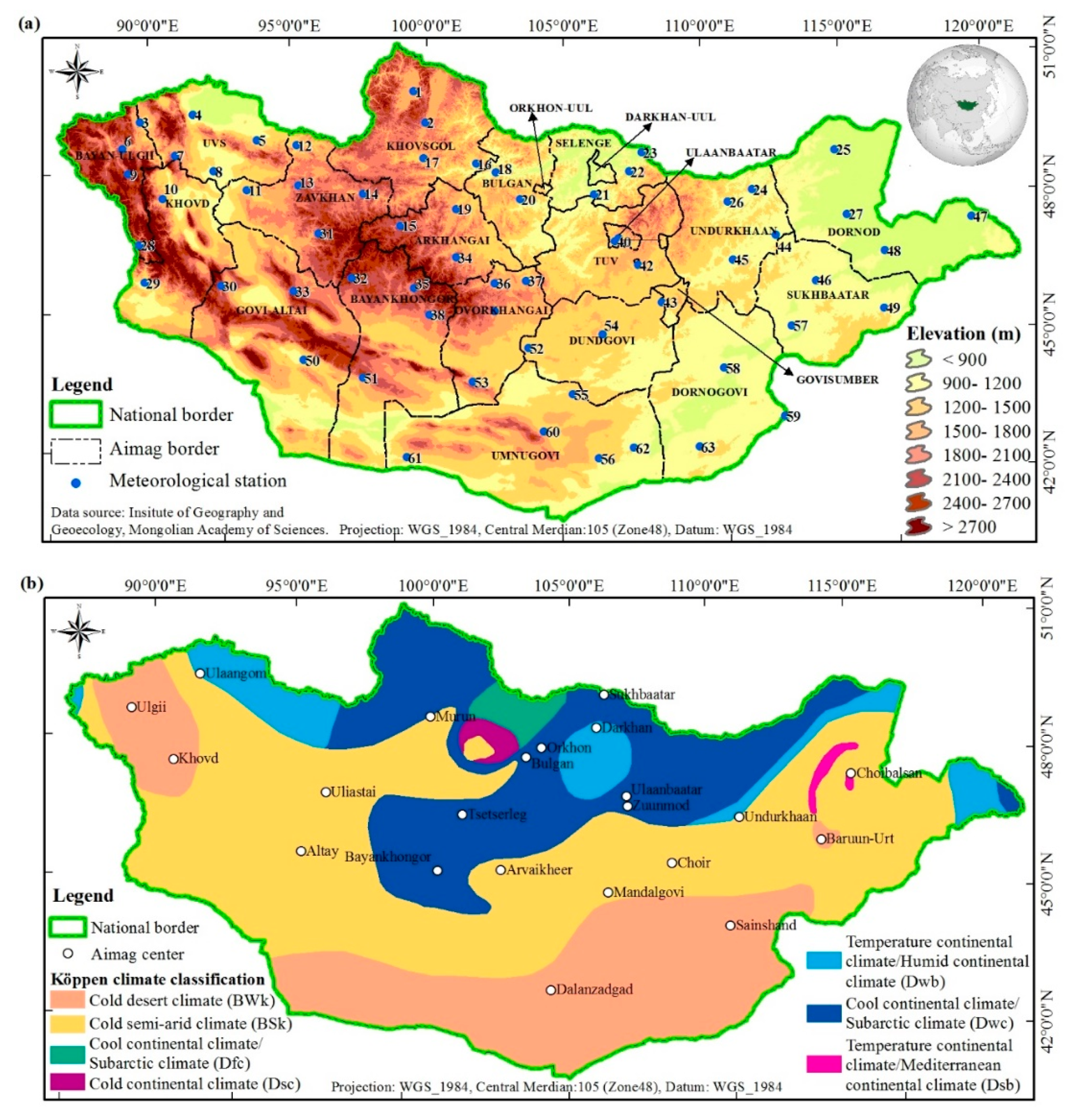
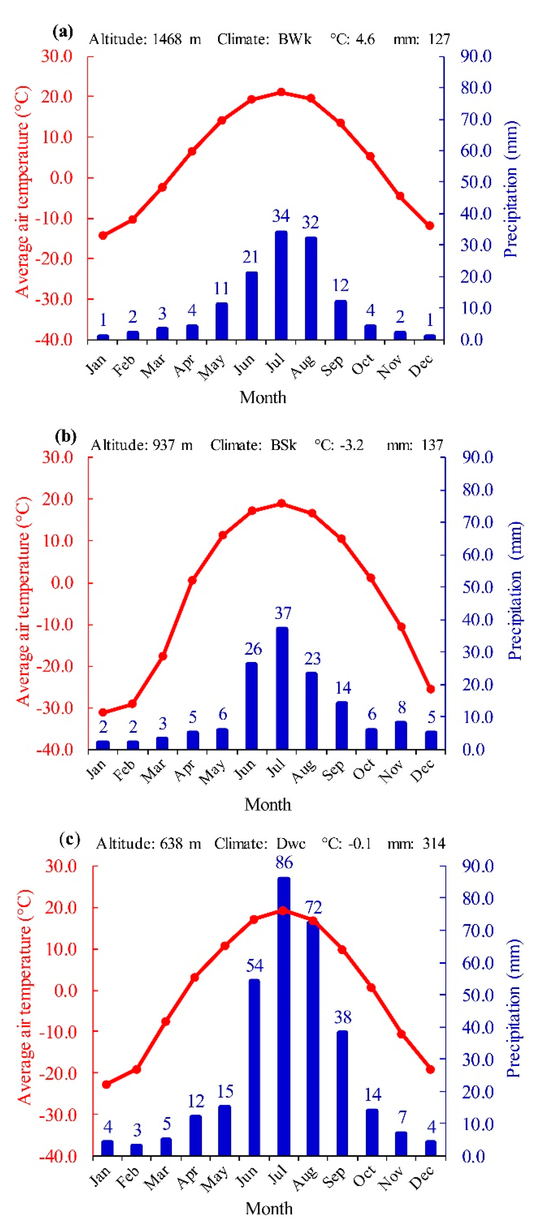
2. Study Area
3. Data and Methods
3.1. Remote Sensing Data
3.2. In Situ Meteorological Data
3.3. Random Forest and Partial Least Square Regression
3.3.1. RF Regression
- Randomly select m variables from p variables
- Pick the variable that best splits and the corresponding split point
- Split the node into two nodes.
3.3.2. PLS Regression
3.3.3. Model Evaluation and Statistics
4. Results
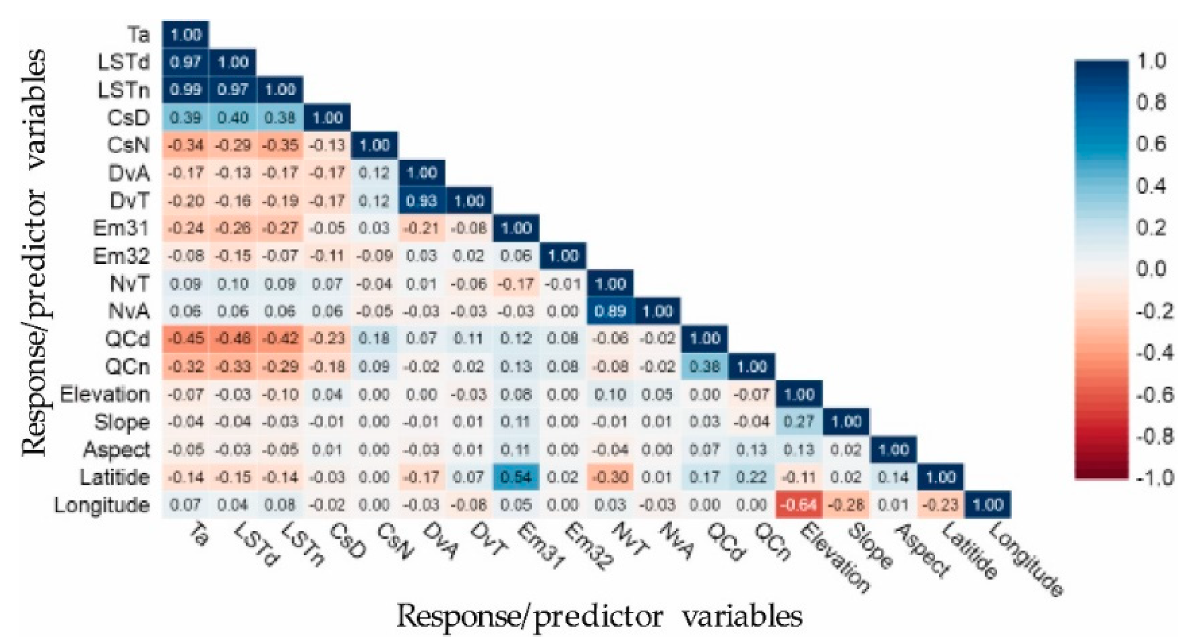
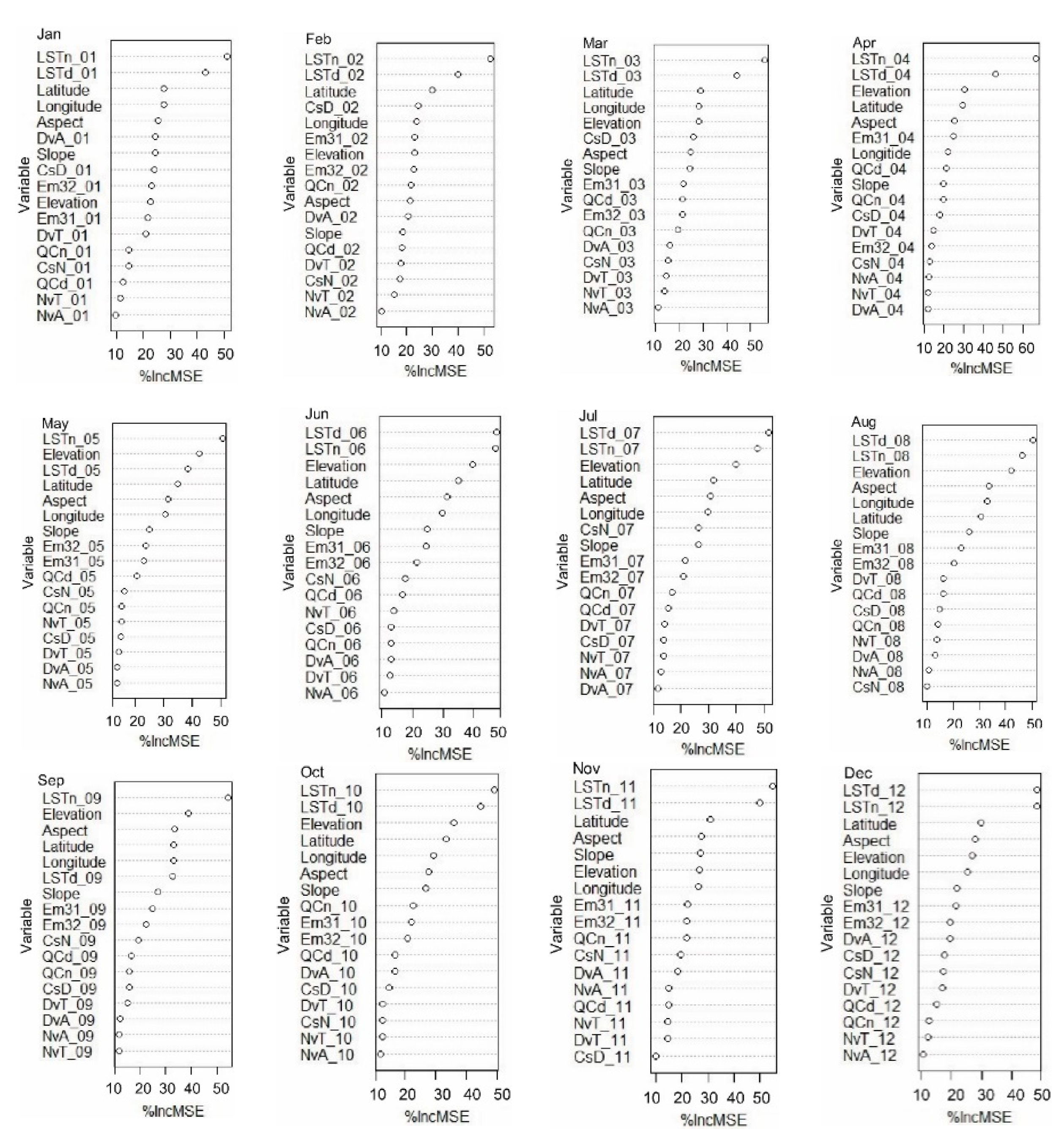
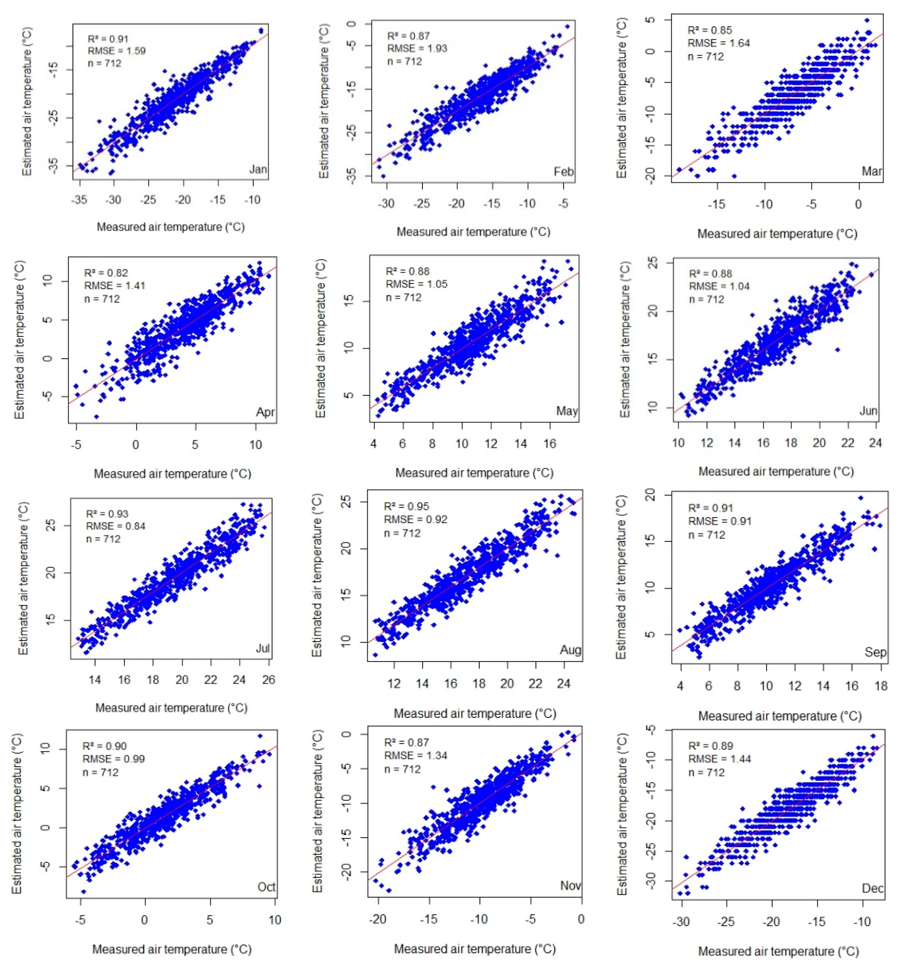
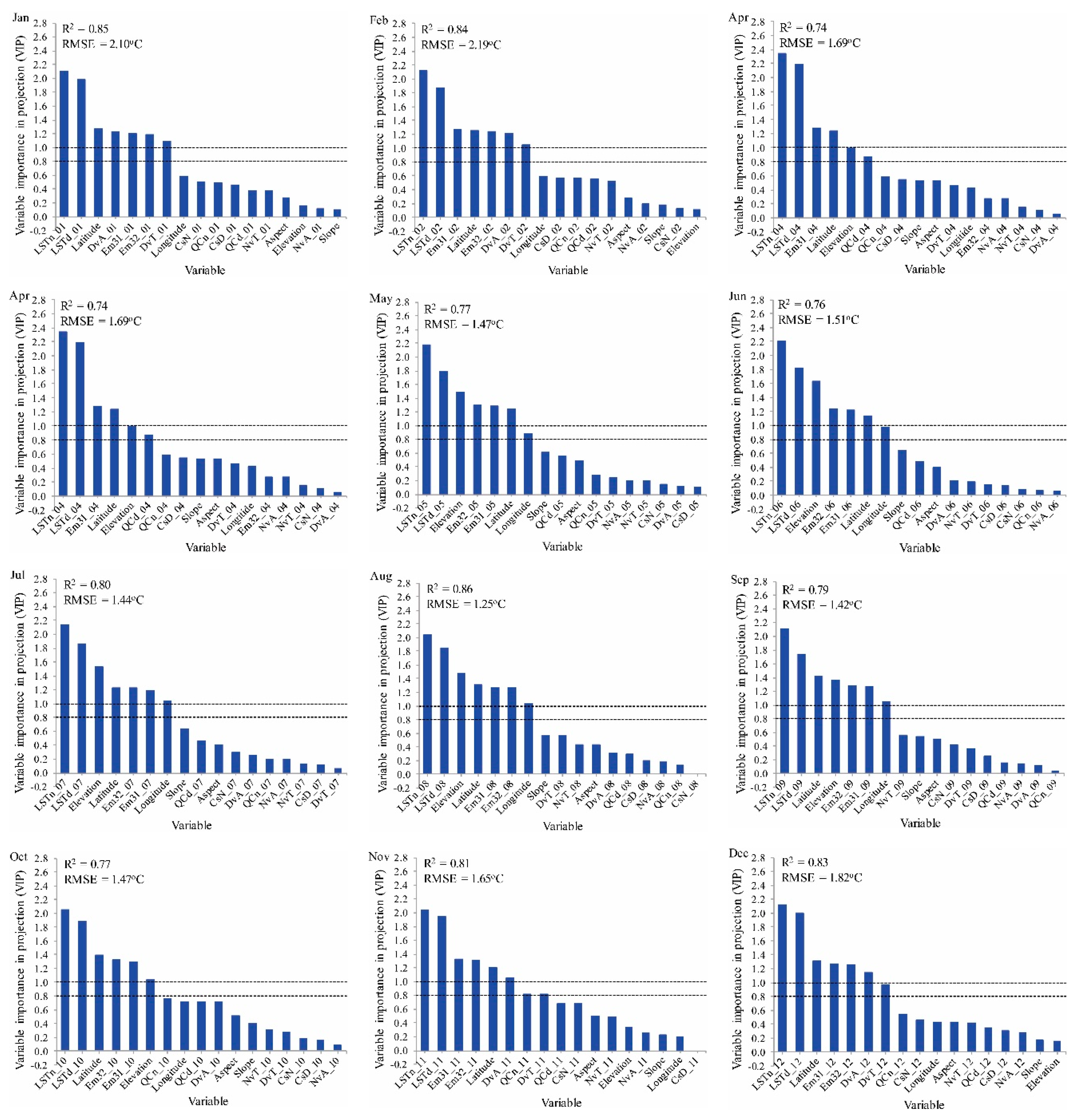
4.1. Comparison of RF and PLS Models: Variable Importance and Prediction Accuracy
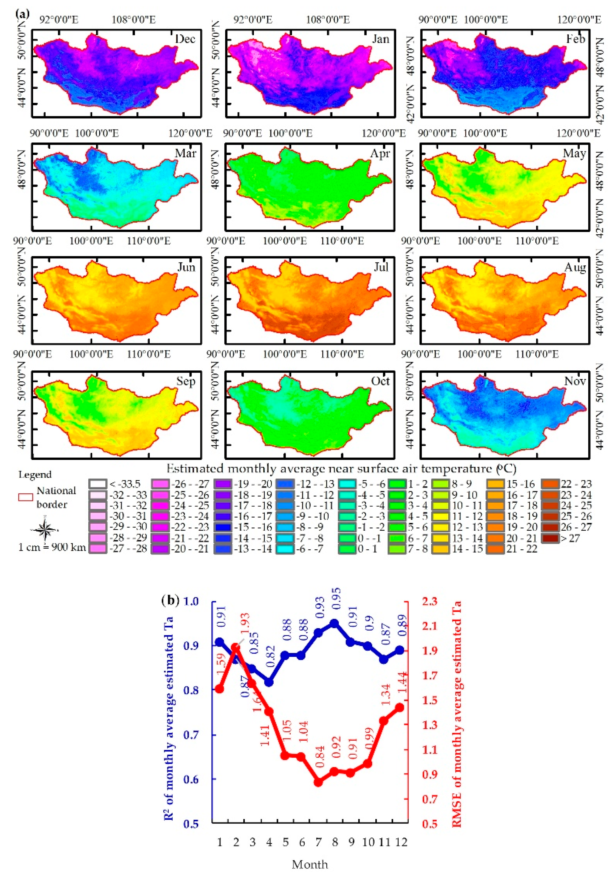
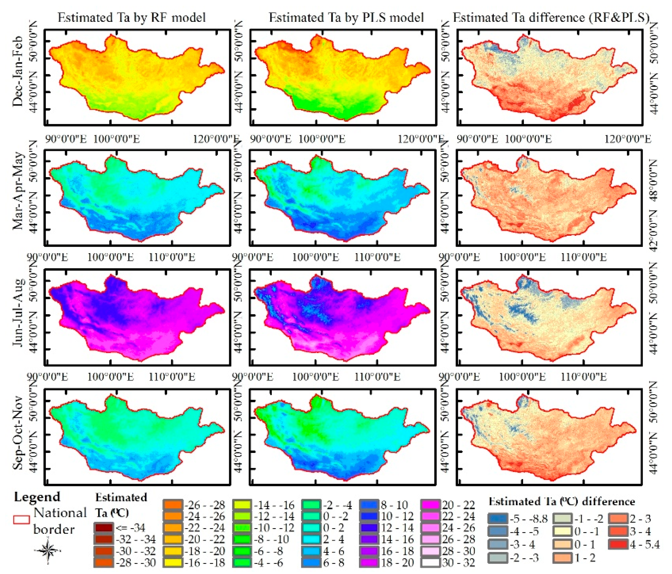
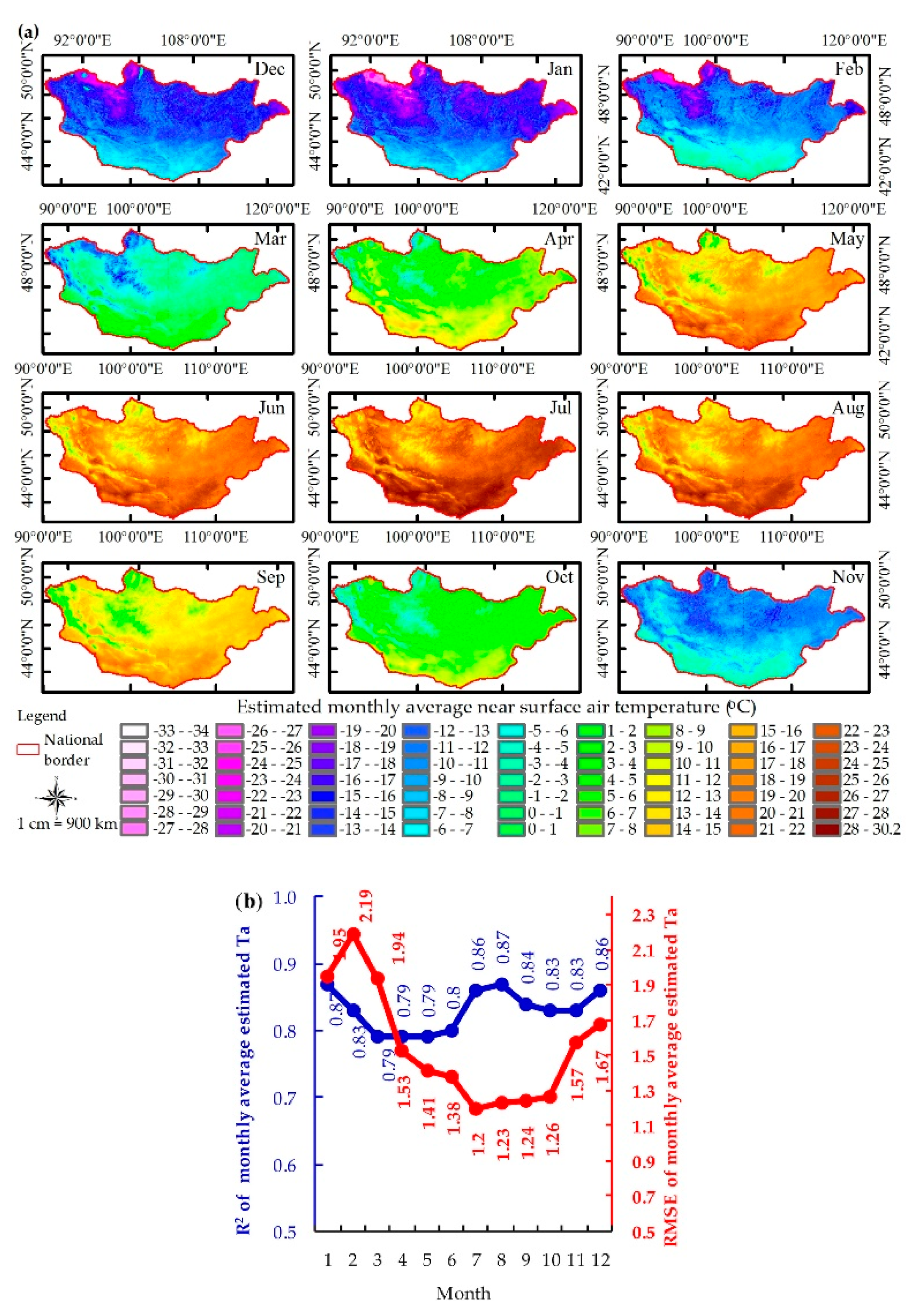
4.2. Maps of Predicted Air Temperatures Using RF Models with the Reduced Feature Set
5. Discussion
6. Conclusions
Author Contributions
Funding
Acknowledgments
Conflicts of Interest
Appendix A


| Variable | Jan | Feb | Mar | Apr | May | Jun | Jul | Aug | Sep | Oct | Nov | Dec | Year |
|---|---|---|---|---|---|---|---|---|---|---|---|---|---|
| Intercept | −52.83 | −93.62 | 26.17 | 55.52 | 93.68 | 89.37 | 97.27 | 45.11 | 68.76 | 62.92 | 53.54 | 22.17 | 82.62 |
| LSTd | 0.255 | 0.219 | 0.208 | 0.185 | 0.159 | 0.146 | 0.137 | 0.178 | 0.150 | 0.128 | 0.197 | 0.234 | 0.319 |
| LSTn | 0.420 | 0.457 | 0.425 | 0.265 | 0.223 | 0.232 | 0.227 | 0.284 | 0.210 | 0.196 | 0.344 | 0.407 | 0.464 |
| CsD | 0.000* | 0.000* | 0.000* | 0.000* | 0.000* | 0.000* | 0.000* | 0.000* | 0.000* | 0.000* | 0.000* | 0.000* | 0.000* |
| CsN | −0.014 | −0.003 | 0.007 | 0.000* | 0.001 | 0.001 | 0.002 | 0.000* | 0.004 | 0.000* | 0.000* | −0.011 | 0.000* |
| DvA | 0.015 | 0.015 | 0.007 | −0.002 | 0.005 | 0.008 | 0.011 | 0.021 | 0.006 | 0.022 | 0.003 | 0.004 | −0.007 |
| DvT | 0.094 | 0.109 | −0.015 | −0.130 | −0.072 | −0.041 | −0.019 | 0.003 | −0.105 | 0.061 | −0.044 | −0.021 | 0.095 |
| Em31 | 0.069 | 0.104 | 0.021 | −0.152 | −0.133 | −0.126 | −0.131 | −0.050 | −0.127 | −0.125 | −0.047 | 0.006 | −0.079 |
| Em32 | 0.101 | 0.158 | 0.003 | −0.012 | −0.208 | −0.198 | −0.209 | −0.096 | −0.199 | −0.195 | −0.087 | −0.009 | 0.007 |
| NvA | −0.019 | −0.034 | −0.034 | −0.012 | −0.009 | −0.002 | −0.007 | −0.017 | 0.007 | −0.004 | −0.017 | −0.028 | −0.038 |
| NvT | 0.031 | 0.100 | −0.114 | 0.045 | 0.053 | 0.050 | 0.034 | 0.029 | 0.169 | 0.083 | −0.030 | −0.038 | −0.413 |
| QCd | 0.000* | 0.000* | 0.000* | 0.000* | 0.000* | 0.000* | 0.000* | 0.000* | 0.000* | 0.000* | 0.000* | 0.000* | 0.000* |
| QCn | 0.000* | 0.000* | 0.000* | 0.000* | 0.000* | 0.000* | 0.000* | 0.000* | 0.000* | 0.000* | 0.000* | 0.000* | 0.000* |
| Elevation | 0.000* | 0.000* | −0.001 | −0.001 | −0.001 | −0.001 | −0.001 | −0.002 | −0.001 | −0.001 | −0.001 | 0.000* | −0.001 |
| Slope | −0.021 | 0.028 | −0.009 | −0.061 | −0.059 | −0.062 | −0.065 | −0.047 | −0.051 | −0.037 | −0.025 | −0.031 | 0.026 |
| Aspect | −0.002 | −0.001 | −0.001 | −0.002 | −0.002 | −0.001 | −0.002 | −0.001 | −0.002 | −0.002 | −0.003 | −0.003 | 0.003 |
| Latitude | −0.411 | −0.401 | −0.248 | −0.268 | −0.236 | −0.214 | −0.246 | −0.244 | −0.260 | −0.248 | −0.241 | −0.393 | 0.336 |
| Longitude | 0.099 | 0.106 | 0.039 | 0.023 | 0.042 | 0.046 | 0.052 | 0.065 | 0.048 | 0.032 | 0.016 | 0.062 | 0.012 |
| n | G1 | G2 | G3 | G4 | G5 | G6 | G7 | ||||||||
|---|---|---|---|---|---|---|---|---|---|---|---|---|---|---|---|
| R2 | RMSE | R2 | RMSE | R2 | RMSE | R2 | RMSE | R2 | RMSE | R2 | RMSE | R2 | RMSE | ||
| January | 712 | 0.87 | 1.96 | 0.87 | 1.95 | 0.34 | 4.34 | 0.82 | 2.26 | 0.39 | 4.17 | 0.86 | 2.01 | 0.85 | 2.10 |
| February | 712 | 0.83 | 2.19 | 0.83 | 2.19 | 0.32 | 4.40 | 0.79 | 2.45 | 0.37 | 4.26 | 0.85 | 2.05 | 0.84 | 2.19 |
| March | 712 | 0.80 | 1.89 | 0.74 | 1.94 | 0.36 | 3.40 | 0.77 | 2.04 | 0.39 | 3.32 | 0.81 | 1.84 | 0.81 | 1.83 |
| April | 712 | 0.79 | 1.51 | 0.79 | 1.53 | 0.48 | 2.39 | 0.77 | 1.58 | 0.32 | 2.73 | 0.75 | 1.67 | 0.74 | 1.69 |
| May | 712 | 0.76 | 1.48 | 0.79 | 1.41 | 0.74 | 1.54 | 0.80 | 1.37 | 0.31 | 2.52 | 0.76 | 1.50 | 0.77 | 1.47 |
| June | 712 | 0.78 | 1.44 | 0.80 | 1.38 | 0.75 | 1.52 | 0.79 | 1.41 | 0.26 | 2.63 | 0.78 | 1.45 | 0.76 | 1.51 |
| July | 712 | 0.83 | 1.33 | 0.86 | 1.20 | 0.79 | 1.48 | 0.84 | 1.28 | 0.28 | 2.71 | 0.82 | 1.34 | 0.80 | 1.44 |
| August | 712 | 0.84 | 1.36 | 0.87 | 1.23 | 0.81 | 1.44 | 0.85 | 1.28 | 0.30 | 2.80 | 0.83 | 1.37 | 0.86 | 1.25 |
| September | 712 | 0.81 | 1.35 | 0.84 | 1.24 | 0.82 | 1.30 | 0.83 | 1.26 | 0.32 | 2.53 | 0.80 | 1.37 | 0.79 | 1.42 |
| October | 712 | 0.83 | 1.27 | 0.83 | 1.26 | 0.68 | 1.73 | 0.82 | 1.31 | 0.41 | 2.36 | 0.81 | 1.32 | 0.77 | 1.47 |
| November | 712 | 0.83 | 1.54 | 0.83 | 1.57 | 0.37 | 2.97 | 0.79 | 1.70 | 0.40 | 2.92 | 0.82 | 1.59 | 0.81 | 1.65 |
| December | 712 | 0.86 | 1.68 | 0.86 | 1.67 | 0.36 | 3.53 | 0.82 | 1.89 | 0.34 | 3.58 | 0.85 | 1.74 | 0.83 | 1.82 |

| Regression Models | R2 | RMSE |
|---|---|---|
| Ta01 = –2.137 + 0.347 × LSTd + 0.497 × LSTn + 0.00033 × elevation | 0.87 | 1.95 |
| Ta02= –3.037 + 0.297 × LSTd + 0.493 × LSTn + 0.00019 × elevation | 0.83 | 2.19 |
| Ta03 = –1.986 + 0.252 × LSTd + 0.477 × LSTn – 0.001 × elevation | 0.74 | 1.94 |
| Ta04 = 0.516 + 0.296 × LSTd + 0.424 × LSTn − 0.002 × elevation | 0.79 | 1.53 |
| Ta05 = 3.863 + 0.272 × LSTd + 0.383 × LSTn − 0.002 × elevation | 0.79 | 1.41 |
| Ta06 = 7.060 + 0.242 × LSTd + 0.384 × LSTn − 0.002 × elevation | 0.80 | 1.38 |
| Ta07 = 8.440 + 0.241 × LSTd + 0.398 × LSTn − 0.002 × elevation | 0.86 | 1.20 |
| Ta08 = 7.644 + 0.253 × LSTd + 0.419 × LSTn − 0.002 × elevation | 0.87 | 1.23 |
| Ta09 = 5.294 + 0.291 × LSTd + 0.407 × LSTn − 0.002 × elevation | 0.84 | 1.24 |
| Ta10 = 3.418 + 0.266 × LSTd + 0.406 × LSTn − 0.002 × elevation | 0.83 | 1.26 |
| Ta11 = –0.912 + 0.271 × LSTd + 0.411 × LSTn − 0.001 × elevation | 0.83 | 1.57 |
| Ta12 = –2.560 + 0.314 × LSTd + 0.463 × LSTn + 0.00037 × elevation | 0.86 | 1.67 |
References
- Nieto, H.; Sandholt, I.; Aguado, I.; Chuvieco, E.; Stisen, S. Air temperature estimation with MSG-SEVIRI data: Calibration and validation of the TVX algorithm for the Iberian Peninsula. Remote Sens. Environ. 2011, 115, 107–116. [Google Scholar] [CrossRef] [Green Version]
- Shamir, E.; Georgakakos, K.P. MODIS Land Surface Temperature as an index of surface air temperature for operational snowpack estimation. Remote Sens. Environ. 2014, 152, 83–98. [Google Scholar] [CrossRef]
- Benali, A.; Carvalho, A.C.; Nunes, J.P.; Carvalhais, N.; Santos, A. Estimating air surface temperature in Portugal using MODIS LST data. Remote Sens. Environ. 2012, 124, 108–121. [Google Scholar] [CrossRef]
- Stisen, S.; Sandholt, I.; Nørgaard, A.; Fensholt, R.; Eklundh, L. Estimation of diurnal air temperature using MSG SEVIRI data in West Africa. Remote Sens. Environ. 2007, 110, 262–274. [Google Scholar] [CrossRef]
- Prihodko, L.; Goward, S.N. Estimation of air temperature from remotely sensed surface observations. Remote Sens. Environ. 1997, 60, 335–346. [Google Scholar] [CrossRef]
- Hooker, J.; Duveiller, G.; Cescatti, A. A global dataset of air temperature derived from satellite remote sensing and weather stations. Sci. Data 2018, 5, 180246. [Google Scholar] [CrossRef] [PubMed] [Green Version]
- Peón, J.; Recondo, C.; Calleja, J.F. Improvements in the estimation of daily minimum air temperature in peninsular Spain using MODIS land surface temperature. Int. J. Remote Sens. 2014, 35, 5148–5166. [Google Scholar] [CrossRef]
- Lam, N.S.N. Spatial interpolation methods: A review. Am. Cartogr. 1983, 10, 129–150. [Google Scholar] [CrossRef]
- Thiébaux, H.J. Statistics and the environment: The analysis of large-scale earth-oriented systems. Environmetrics 1991, 2, 5–24. [Google Scholar] [CrossRef]
- Ishida, T.; Kawashima, S. Use of cokriging to estimate surface air temperature from elevation. Theor. Appl. Clim. 1993, 47, 147–157. [Google Scholar] [CrossRef]
- Hutchinson, M.F. A New Objective Method for Spatial Interpolation of Meteorological Variables from Irregular Networks Applied to the Estimation of Monthly Mean Solar Radiation, Temperature, Precipitation and Windrun; Need for climatic and hydrologic data in agriculture in South East Asia; UN University Workshop: Canberra, Australia, 1983; pp. 95–104. [Google Scholar]
- Willmott, C.J.; Rowe, C.M.; Philpot, W.D. Small-Scale Climate Maps: A Sensitivity Analysis of Some Common Assumptions Associated with Grid-Point Interpolation and Contouring. Am. Cartogr. 1985, 12, 5–16. [Google Scholar] [CrossRef]
- Willmott, C.J.; Robeson, S.M. Climatologically aided interpolation (CAI) of terrestrial air temperature. Int. J. Clim. 1995, 15, 221–229. [Google Scholar] [CrossRef]
- Burrough, P.A.; McDonnell, R.A. Principles of Geographical Information Systems; Oxford University Press: Oxford, UK, 1998. [Google Scholar]
- Mostovoy, G.V.; King, R.L.; Reddy, K.R.; Kakani, V.G.; Filippova, M.G. Statistical Estimation of Daily Maximum and Minimum Air Temperatures from MODIS LST Data over the State of Mississippi. GIScience Remote Sens. 2006, 43, 78–110. [Google Scholar] [CrossRef] [Green Version]
- Vogt, J.V.; Viau, A.A.; Paquet, F. Mapping regional air temperature fields using satellite-derived surface skin temperatures. Int. J. Clim. 1997, 17, 1559–1579. [Google Scholar] [CrossRef]
- Vancutsem, C.; Ceccato, P.; Dinku, T.; Connor, S.J. Evaluation of MODIS land surface temperature data to estimate air temperature in different ecosystems over Africa. Remote Sens. Environ. 2010, 114, 449–465. [Google Scholar] [CrossRef]
- Dash, P.; Göttsche, F.-M.; Olesen, F.-S.; Fischer, H. Land surface temperature and emissivity estimation from passive sensor data: Theory and practice-current trends. Int. J. Remote Sens. 2002, 23, 2563–2594. [Google Scholar] [CrossRef]
- Oke, T. The urban energy balance. Prog. Phys. Geogr. Earth Environ. 1988, 12, 471–508. [Google Scholar] [CrossRef]
- Chatterjee, R.; Singh, N.; Thapa, S.; Sharma, D.; Kumar, D. Retrieval of land surface temperature (LST) from landsat TM6 and TIRS data by single channel radiative transfer algorithm using satellite and ground-based inputs. Int. J. Appl. Earth Obs. Geoinf. 2017, 58, 264–277. [Google Scholar] [CrossRef]
- Li, Z.-L.; Tang, B.-H.; Wu, H.; Ren, H.; Yan, G.; Wan, Z.; Trigo, I.F.; Sobrino, J.A. Satellite-derived land surface temperature: Current status and perspectives. Remote Sens. Environ. 2013, 131, 14–37. [Google Scholar] [CrossRef] [Green Version]
- Prata, A.J.; Caselles, V.; Coll, C.; Sobrino, J.A.; Ottlé, C. Thermal remote sensing of land surface temperature from satellites: Current status and future prospects. Remote Sens. Rev. 1995, 12, 175–224. [Google Scholar] [CrossRef]
- Cresswell, M.P.; Morse, A.P.; Thomson, M.C.; Connor, S.J. Estimating surface air temperatures, from Meteosat land surface temperatures, using an empirical solar zenith angle model. Int. J. Remote Sens. 1999, 20, 1125–1132. [Google Scholar] [CrossRef]
- Stoll, M.J.; Brazel, A.J. Surface-air temperature relationships in the urban environment of phoenix, Arizona. Phys. Geogr. 1992, 13, 160–179. [Google Scholar] [CrossRef]
- Garand, L.; Buehner, M.; Wagneur, N. Background Error Correlation between Surface Skin and Air Temperatures: Estimation and Impact on the Assimilation of Infrared Window Radiances. J. Appl. Meteorol. 2004, 43, 1853–1863. [Google Scholar] [CrossRef]
- Jin, M.; Dickinson, R.E. Land surface skin temperature climatology: Benefitting from the strengths of satellite observations. Environ. Res. Lett. 2010, 5, 044004. [Google Scholar] [CrossRef]
- Zakšek, K.; Schroedter-Homscheidt, M. Parameterization of air temperature in high temporal and spatial resolution from a combination of the SEVIRI and MODIS instruments. ISPRS J. Photogramm. Remote Sens. 2009, 64, 414–421. [Google Scholar] [CrossRef]
- Sun, Y.J.; Wang, J.F.; Zhang, R.H.; Gillies, R.R.; Xue, Y.Y.C.B.; Bo, Y.C. Air temperature retrieval from remote sensing data based on thermodynamics. Theor. Appl. Climatol. 2005, 80, 37–48. [Google Scholar] [CrossRef]
- Zhu, W.; Lű, A.; Jia, S. Estimation of daily maximum and minimum air temperature using MODIS land surface temperature products. Remote Sens. Environ. 2013, 130, 62–73. [Google Scholar] [CrossRef]
- Czajkowski, K.; Goward, S.; Stadler, S.; Walz, A. Thermal Remote Sensing of Near Surface Environmental Variables: Application Over the Oklahoma Mesonet. Prof. Geogr. 2000, 52, 345–357. [Google Scholar] [CrossRef]
- Kilibarda, M.; Hengl, T.; Heuvelink, G.B.M.; Gräler, B.; Pebesma, E.; Tadić, M.P.; Bajat, B. Spatio-temporal interpolation of daily temperatures for global land areas at 1 km resolution. J. Geophys. Res. Atmos. 2014, 119, 2294–2313. [Google Scholar] [CrossRef]
- Chen, F.; Liu, Y.; Liu, Q.; Qin, F. A statistical method based on remote sensing for the estimation of air temperature in China. Int. J. Climatol. 2015, 35, 2131–2143. [Google Scholar] [CrossRef]
- Xu, Y.; Qin, Z.; Shen, Y. Study on the estimation of near-surface air temperature from MODIS data by statistical methods. Int. J. Remote Sens. 2012, 33, 7629–7643. [Google Scholar] [CrossRef]
- Yan, H.; Zhang, J.; Hou, Y.; He, Y. Estimation of air temperature from MODIS data in east China. Int. J. Remote Sens. 2009, 30, 6261–6275. [Google Scholar] [CrossRef]
- Bartkowiak, P.; Castelli, M.; Notarnicola, C. Downscaling Land Surface Temperature from MODIS Dataset with Random Forest Approach over Alpine Vegetated Areas. Remote Sens. 2019, 11, 1319. [Google Scholar] [CrossRef]
- Lu, L.; Zhang, T.; Wang, T.; Zhou, X. Evaluation of Collection-6 MODIS Land Surface Temperature Product Using Multi-Year Ground Measurements in an Arid Area of Northwest China. Remote Sens. 2018, 10, 1852. [Google Scholar] [CrossRef]
- Zhou, W.; Peng, B.; Shi, J.; Wang, T.; Dhital, Y.P.; Yao, R.; Yu, Y.; Lei, Z.; Zhao, R. Estimating High Resolution Daily Air Temperature Based on Remote Sensing Products and Climate Reanalysis Datasets over Glacierized Basins: A Case Study in the Langtang Valley, Nepal. Remote Sens. 2017, 9, 959. [Google Scholar] [CrossRef]
- Janatian, N.; Sadeghi, M.; Sanaeinejad, S.H.; Bakhshian, E.; Farid, A.; Hasheminia, S.M.; Ghazanfari, S. A statistical framework for estimating air temperature using MODIS land surface temperature data. Int. J. Climatol. 2017, 37, 1181–1194. [Google Scholar] [CrossRef]
- Ho, H.C.; Knudby, A.; Sirovyak, P.; Xu, Y.; Hodul, M.; Henderson, S.B. Mapping maximum urban air temperature on hot summer days. Remote Sens. Environ. 2014, 154, 38–45. [Google Scholar] [CrossRef]
- Duan, S.-B.; Li, Z.-L.; Tang, B.-H.; Wu, H.; Tang, R.; Bi, Y.; Zhou, G. Estimation of Diurnal Cycle of Land Surface Temperature at High Temporal and Spatial Resolution from Clear-Sky MODIS Data. Remote Sens. 2014, 6, 3247–3262. [Google Scholar] [CrossRef] [Green Version]
- Noi, P.T.; Kappas, M.; Degener, J. Estimating Daily Maximum and Minimum Land Air Surface Temperature Using MODIS Land Surface Temperature Data and Ground Truth Data in Northern Vietnam. Remote Sens. 2016, 8, 1002. [Google Scholar] [CrossRef]
- Li, L.; Zha, Y. Estimating monthly average temperature by remote sensing in China. Adv. Space Res. 2019, 63, 2345–2357. [Google Scholar] [CrossRef]
- Yoo, C.; Im, J.; Park, S.; Quackenbush, L.J. Estimation of daily maximum and minimum air temperatures in urban landscapes using MODIS time series satellite data. ISPRS J. Photogramm. Remote Sens. 2018, 137, 149–162. [Google Scholar] [CrossRef]
- Yang, Y.Z.; Cai, W.H.; Yang, J. Evaluation of MODIS Land Surface Temperature Data to Estimate Near-Surface Air Temperature in Northeast China. Remote Sens. 2017, 9, 410. [Google Scholar] [CrossRef]
- Meyer, H.; Katurji, M.; Appelhans, T.; Müller, M.U.; Nauss, T.; Roudier, P.; Zawar-Reza, P. Mapping Daily Air Temperature for Antarctica Based on MODIS LST. Remote Sens. 2016, 8, 732. [Google Scholar] [CrossRef]
- Emamifar, S.; Rahimikhoob, A.; Noroozi, A.A. Daily mean air temperature estimation from MODIS land surface temperature products based on M5 model tree. Int. J. Clim. 2013, 33, 3174–3181. [Google Scholar] [CrossRef]
- Zhang, H.; Zhang, F.; Zhang, G.; He, X.; Tian, L. Evaluation of cloud effects on air temperature estimation using MODIS LST based on ground measurements over the Tibetan Plateau. Atmos. Chem. Phys. Discuss. 2016, 16, 13681–13696. [Google Scholar] [CrossRef] [Green Version]
- Keramitsoglou, I.; Kiranoudis, C.T.; Sismanidis, P.; Zakšek, K. An Online System for Nowcasting Satellite Derived Temperatures for Urban Areas. Remote Sens. 2016, 8, 306. [Google Scholar] [CrossRef]
- Nanzad, L.; Zhang, J.; Tuvdendorj, B.; Nabil, M.; Zhang, S.; Bai, Y. NDVI anomaly for drought monitoring and its correlation with climate factors over Mongolia from 2000 to 2016. J. Arid. Environ. 2019, 164, 69–77. [Google Scholar] [CrossRef]
- Nandintsetseg, B.; Greene, J.S.; Goulden, C.E. Trends in extreme daily precipitation and temperature near lake Hövsgöl, Mongolia. Int. J. Clim. 2007, 27, 341–347. [Google Scholar] [CrossRef]
- World Map of the Köppen Climate Classification. Available online: https://commons.wikimedia.org/wiki/File:World_K%C3%B6ppen_Classification_(with_authors).svg (accessed on 18 October 2019).
- Climate Data Org Webpage. Available online: https://en.climate-data.org/asia/mongolia-180/ (accessed on 17 October 2019).
- Duan, S.-B.; Li, Z.-L.; Wu, H.; Leng, P.; Gao, M.; Wang, C. Radiance-based validation of land surface temperature products derived from Collection 6 MODIS thermal infrared data. Int. J. Appl. Earth Obs. Geoinf. 2018, 70, 84–92. [Google Scholar] [CrossRef]
- Oyler, J.W.; Dobrowski, S.Z.; Holden, Z.A.; Running, S.W. Remotely Sensed Land Skin Temperature as a Spatial Predictor of Air Temperature across the Conterminous United States. J. Appl. Meteorol. Clim. 2016, 55, 1441–1457. [Google Scholar] [CrossRef]
- Xu, Y.; Knudby, A.; Ho, H.C. Estimating daily maximum air temperature from MODIS in British Columbia, Canada. Int. J. Remote Sens. 2014, 35, 8108–8121. [Google Scholar] [CrossRef]
- Wan, Z.; Dozier, J. A generalized split-window algorithm for retrieving land-surface temperature from space. IEEE Trans. Geosci. Remote Sens. 1996, 34, 892–905. [Google Scholar] [Green Version]
- Wan, Z. New refinements and validation of the MODIS Land-Surface Temperature/Emissivity products. Remote Sens. Environ. 2008, 112, 59–74. [Google Scholar] [CrossRef]
- Wan, Z. New refinements and validation of the collection-6 MODIS land-surface temperature/emissivity product. Remote Sens. Environ. 2014, 140, 36–45. [Google Scholar] [CrossRef]
- Wan, Z.; Zhang, Y.; Zhang, Q.; Li, Z.-L. Validation of the land-surface temperature products retrieved from Terra Moderate Resolution Imaging Spectroradiometer data. Remote Sens. Environ. 2002, 83, 163–180. [Google Scholar] [CrossRef]
- Wan, Z. Collection-6 MODIS Land Surface Temperature Products Users’ Guide; ICESS: Santa Barbara, CA, USA, 2007. [Google Scholar]
- Mattiuzzi, M.; Verbesselt, J.; Klisch, A.; Stevens, F.; Mosher, S.; Evans, B.; Lobo, A.; Detsch, F. MODIS: MODIS Acquisition and Processing Package. R Package Version 1.1.4. Available online: https://cran.r-project.org/src/contrib/Archive/MODIS/MODIS.pdf (accessed on 25 October 2018).
- R Core Team. R: A Language and Environment for Statistical Computing. Available online: https://www.R-project.org/ (accessed on 31 October 2019).
- Mattiuzzi, M.; Verbesselt, J.; Hengel, T.; Klisch, A.; Stevens, F.; Mosher, S.; Evans, B.; Lobo, A.; Hufkens, K.; Detsch, F. MODIS: MODIS Acquisition and Processing package. R Package Version 1.1.5. Available online: https://cran.r-project.org/web/packages/MODIS/MODIS.pdf (accessed on 8 March 2019).
- Rabus, B.; Eineder, M.; Roth, A.; Bamler, R. The shuttle radar topography mission—A new class of digital elevation models acquired by spaceborne radar. ISPRS J. Photogramm. Remote Sens. 2003, 57, 241–262. [Google Scholar] [CrossRef]
- Bulgan, D.; Mandakh, N.; Odbayar, M.; Otgontugs, M.; Tsogtbaatar, J.; Elbegjargal, N.; Enerel, T.; Erdenetuya, M. Desertification Atlas of Mongolia; Tsogtbaatar, J., Khudulmur, S., Eds.; Admon Press: Ulaanbaatar, Mongolia, 2013; pp. 17–29. ISBN 978-9973-0-065-2. [Google Scholar]
- Breiman, L. Random forests. Mach. Learn. 2001, 45, 5–32. [Google Scholar] [CrossRef]
- Mutanga, O.; Adam, E.; Cho, M.A. High density biomass estimation for wetland vegetation using WorldView-2 imagery and random forest regression algorithm. Int. J. Appl. Earth Obs. Geoinf. 2012, 18, 399–406. [Google Scholar] [CrossRef]
- Pal, M. Random forest classifier for remote sensing classification. Int. J. Remote Sens. 2005, 26, 217–222. [Google Scholar] [CrossRef]
- Liaw, A.; Wiener, M. Classification and regression by randomForest. R News 2002, 2, 18–22. [Google Scholar]
- Immitzer, M.; Stepper, C.; Bock, S.; Straub, C.; Atzberger, C. Use of WorldView-2 stereo imagery and National Forest Inventory data for wall-to-wall mapping of growing stock. For. Ecol. Manag. 2016, 359, 232–246. [Google Scholar] [CrossRef]
- Belgiu, M.; Drăguț, L. Random forest in remote sensing: A review of applications and future directions. ISPRS J. Photogramm. Remote Sens. 2016, 114, 24–31. [Google Scholar] [CrossRef]
- Hudak, A.T.; Crookston, N.L.; Evans, J.S.; Hall, D.E.; Falkowski, M.J. Nearest neighbor imputation of species-level, plot-scale forest structure attributes from LiDAR data. Remote Sens. Environ. 2008, 112, 2232–2245. [Google Scholar] [CrossRef] [Green Version]
- Rodriguez-Galiano, V.F.; Ghimire, B.; Rogan, J.; Olmo, M.C.; Rigol-Sanchez, J.P. An assessment of the effectiveness of a random forest classifier for land-cover classification. ISPRS J. Photogramm. Remote Sens. 2012, 67, 93–104. [Google Scholar] [CrossRef]
- Genuer, R.; Poggi, J.-M.; Tuleau-Malot, C. Variable selection using random forests. Pattern Recognit. Lett. 2010, 31, 2225–2236. [Google Scholar] [CrossRef] [Green Version]
- Trevor, H.; Tibshirani, R.; Friedman, J. The Elements of Statistical Learning; Springer: Stanford, CA, USA, 2011. [Google Scholar]
- Prasad, A.M.; Iverson, L.R.; Liaw, A. Newer Classification and Regression Tree Techniques: Bagging and Random Forests for Ecological Prediction. Ecosystems 2006, 9, 181–199. [Google Scholar] [CrossRef]
- Ishwaran, H. Variable importance in binary regression trees and forests. Electron. J. Stat. 2007, 1, 519–537. [Google Scholar] [CrossRef]
- Atzberger, C.; Guérif, M.; Baret, F.; Werner, W. Comparative analysis of three chemometric techniques for the spectroradiometric assessment of canopy chlorophyll content in winter wheat. Comput. Electron. Agric. 2010, 73, 165–173. [Google Scholar] [CrossRef]
- Laurin, G.V.; Chen, Q.; Lindsell, J.A.; Coomes, D.A.; Del Frate, F.; Guerriero, L.; Pirotti, F.; Valentini, R. Above ground biomass estimation in an African tropical forest with lidar and hyperspectral data. ISPRS J. Photogramm. Remote Sens. 2014, 89, 49–58. [Google Scholar] [CrossRef]
- Inoue, Y.; Sakaiya, E.; Zhu, Y.; Takahashi, W. Diagnostic mapping of canopy nitrogen content in rice based on hyperspectral measurements. Remote Sens. Environ. 2012, 126, 210–221. [Google Scholar] [CrossRef]
- Gomez, C.; Rossel, R.A.V.; McBratney, A.B. Soil organic carbon prediction by hyperspectral remote sensing and field vis-NIR spectroscopy: An Australian case study. Geoderma 2008, 146, 403–411. [Google Scholar] [CrossRef]
- Farifteh, J.; Van Der Meer, F.; Atzberger, C.; Carranza, E.; Carranza, E.J. Quantitative analysis of salt-affected soil reflectance spectra: A comparison of two adaptive methods (PLSR and ANN). Remote Sens. Environ. 2007, 110, 59–78. [Google Scholar] [CrossRef]
- Rossel, R.V.; Walvoort, D.; McBratney, A.; Janik, L.; Skjemstad, J.; Rossel, R.V. Visible, near infrared, mid infrared or combined diffuse reflectance spectroscopy for simultaneous assessment of various soil properties. Geoderma 2006, 131, 59–75. [Google Scholar] [CrossRef]
- Fernandes, L.S.; Fernandes, A.; Ferreira, A.; Cortes, R.; Pacheco, F. A partial least squares—Path modeling analysis for the understanding of biodiversity loss in rural and urban watersheds in Portugal. Sci. Total Environ. 2018, 626, 1069–1085. [Google Scholar] [CrossRef] [PubMed]
- Liu, Y.; Peng, J.; Wang, Y. Application of partial least squares regression in detecting the important landscape indicators determining urban land surface temperature variation. Landsc. Ecol. 2018, 33, 1133–1145. [Google Scholar] [CrossRef]
- Ceglar, A.; Toreti, A.; Lecerf, R.; Van Der Velde, M.; Dentener, F. Impact of meteorological drivers on regional inter-annual crop yield variability in France. Agric. For. Meteorol. 2016, 216, 58–67. [Google Scholar] [CrossRef]
- Carrascal, L.M.; Galván, I.; Gordo, O. Partial least squares regression as an alternative to current regression methods used in ecology. Oikos 2009, 118, 681–690. [Google Scholar] [CrossRef]
- Abdi, H. Partial least square regression (PLS regression). Encycl. Res. Methods Soc. Sci. 2003, 6, 1–7. [Google Scholar]
- Wold, H. Soft modeling: The basic design and some extensions. Syst. Indirect Obs. 1982, 2, 343. [Google Scholar]
- Wold, S.; Sjöström, M.; Eriksson, L. PLS-regression: A basic tool of chemometrics. Chemom. Intell. Lab Syst. 2001, 58, 109–130. [Google Scholar] [CrossRef]
- Geladi, P.; Kowalski, B.R. Partial least-squares regression: A tutorial. Anal. Chim. Acta 1986, 185, 1–17. [Google Scholar] [CrossRef]
- Mevik, B.; Cederkvist, H.R. Mean squared error of prediction (MSEP) estimates for principal component regression (PCR) and partial least squares regression (PLSR). J. Chemom. 2004, 18, 422–429. [Google Scholar] [CrossRef]
- Mkhabela, M.S.; Bullock, P.R.; Sapirstein, H.D. Characterising the most critical climatic parameters that impact the quality of spring-wheat (Triticum aestivum L.) on the Canadian Prairies using partial least squares (PLS) analysis. J. Cereal Sci. 2018, 81, 44–51. [Google Scholar] [CrossRef]
- Richter, K.; Atzberger, C.; Hank, T.B.; Mauser, W. Derivation of biophysical variables from Earth observation data: Validation and statistical measures. J. Appl. Remote Sens. 2012, 6, 63557. [Google Scholar] [CrossRef]
- Farres, M.; Platikanov, S.; Tsakovski, S.; Tauler, R. Comparison of the variable importance in projection (VIP) and of the selectivity ratio (SR) methods for variable selection and interpretation. J. Chemom. 2015, 29, 528–536. [Google Scholar] [CrossRef]
- Otgonbayar, M.; Atzberger, C.; Chambers, J.; Damdinsuren, A. Mapping pasture biomass in Mongolia using Partial Least Squares, Random Forest regression and Landsat 8 imagery. Int. J. Remote Sens. 2019, 40, 3204–3226. [Google Scholar] [CrossRef]
- Sun, J.; Passi, K.; Jain, C.K. Improved microarray data analysis using feature selection methods with machine learning methods. In Proceedings of the 2016 IEEE International Conference on Bioinformatics and Biomedicine (BIBM), Shenzhen, China, 15–18 December 2016; pp. 1527–1534. [Google Scholar]


| Variable Type | Acronym | Units | Data Type | Fill Value | Valid Range (VR) | Scale Factor (SF) | Additional Offset (AO) |
|---|---|---|---|---|---|---|---|
| Daytime LST | LSTd | Kelvin | 16 bit | 0 | 7500 to 65,535 | 0.02 | N/A |
| Nighttime LST | LSTn | Kelvin | 16 bit | 0 | 7500 to 65,535 | 0.02 | N/A |
| Day clear sky coverage | CsD | N/A | 16 bit | 0 | 1 to 65,535 | 0.0005 | N/A |
| Night clear sky coverage | CsN | N/A | 16 bit | 0 | 1 to 65,535 | 0.0005 | N/A |
| View zenith angle of daytime | DvA | Degree | 8 bit | 255 | 0 to 130 | 1.0 | −65 |
| View zenith angle of nighttime | NvA | Degree | 8 bit | 255 | 0 to 130 | 1.0 | −65 |
| Time of daytime (local solar) | DvT | Hours | 8 bit | 255 | 0 to 240 | 0.1 | N/A |
| Time of nighttime (local solar) | NvT | Hours | 8 bit | 255 | 0 to 240 | 0.1 | N/A |
| Emissivity band 31 | Em31 | None | 8 bit | 0 | 1 to 255 | 0.002 | 0.49 |
| Emissivity band 32 | Em32 | None | 8 bit | 0 | 1 to 255 | 0.002 | 0.49 |
| Quality controls of day LST | QCd | Bit | 8 bit | N/A | 0 to 255 | N/A | N/A |
| Quality controls of night LST | QCn | Bit | 8 bit | N/A | 0 to 255 | N/A | N/A |
| Variable | No. of Samples (n) | Minimum | Maximum | Mean | Standard Deviation |
|---|---|---|---|---|---|
| Ta01 | 712 | −36.60 | −6.60 | −20.83 | 5.36 |
| Ta02 | 712 | −35.10 | −0.60 | −16.60 | 5.38 |
| Ta03 | 712 | −20.50 | 4.80 | −6.73 | 4.22 |
| Ta04 | 712 | −7.60 | 12.40 | 3.92 | 3.32 |
| Ta05 | 712 | 2.80 | 19.30 | 10.75 | 3.05 |
| Ta06 | 712 | 9.20 | 24.90 | 16.98 | 3.06 |
| Ta07 | 712 | 11.60 | 27.20 | 19.49 | 3.21 |
| Ta08 | 712 | 8.70 | 25.60 | 17.16 | 3.34 |
| Ta09 | 712 | 2.60 | 19.70 | 10.48 | 3.07 |
| Ta10 | 712 | −8.20 | 11.70 | 1.49 | 3.08 |
| Ta11 | 712 | −22.70 | 0.30 | −9.62 | 3.76 |
| Ta12 | 712 | −31.50 | −6.10 | −17.85 | 4.40 |
| LSTd | 8544 | −36.90 | 48.60 | 13.43 | 20.08 |
| LSTn | 8544 | −42.50 | 24.40 | −5.75 | 14.47 |
| CsD | 8544 | 0.00 | 0.13 | 0.06 | 0.02 |
| CsN | 8544 | 0.00 | 0.13 | 0.07 | 0.02 |
| DvA | 8544 | −55.00 | 62.00 | 5.04 | −52.35 |
| DvT | 8544 | 10.40 | 12.10 | 11.82 | 0.71 |
| Em31 | 8544 | 0.96 | 0.99 | 0.98 | 0.50 |
| Em32 | 8544 | 0.97 | 0.99 | 0.98 | 0.49 |
| NvA | 8544 | −65.00 | 56.00 | −0.48 | −56.47 |
| NvT | 8544 | 20.80 | 22.70 | 21.90 | 1.29 |
| QCd | 8544 | 2.00 | 133.00 | 61.98 | 16.58 |
| QCn | 8544 | 2.00 | 145.00 | 55.14 | 19.70 |
| Elevation | 63 | 667.00 | 2255.00 | 1369.10 | 411.70 |
| Slope | 63 | 0.08 | 19.60 | N/A | N/A |
| Aspect | 63 | 6.34 | 358.10 | N/A | N/A |
| Latitude | 63 | 42.97 | 51.11 | N/A | N/A |
| Longitude | 63 | 89.93 | 118.67 | N/A | N/A |
| Acronym | Variables | Nvar | |
|---|---|---|---|
| Group 1 | G1 | LSTd and LSTn | 2 |
| Group 2 | G2 | LSTd, LSTn, and elevation | 3 |
| Group 3 | G3 | Elevation, slope, aspect, latitude, and longitude | 5 |
| Group 4 | G4 | Combined G1 and G3 | 7 |
| Group 5 | G5 | CsD, CsN, DvA, DvT, Em31, Em32, NvA, NvT, QCd, and QCn | 10 |
| Group 6 | G6 | Combined G1 and G5 | 12 |
| Group 7 | G7 | Combined G1, G3, and G5 | 17 |
| n | G1 | G2 | G3 | G4 | G5 | G6 | G7 | ||||||||
|---|---|---|---|---|---|---|---|---|---|---|---|---|---|---|---|
| R2 | RMSE | R2 | RMSE | R2 | RMSE | R2 | RMSE | R2 | RMSE | R2 | RMSE | R2 | RMSE | ||
| January | 712 | 0.85 | 2.07 | 0.91 | 1.59 | 0.52 | 3.71 | 0.89 | 1.77 | 0.40 | 4.14 | 0.88 | 1.86 | 0.90 | 1.71 |
| February | 712 | 0.83 | 2.24 | 0.87 | 1.93 | 0.49 | 3.83 | 0.86 | 2.05 | 0.46 | 3.95 | 0.85 | 2.06 | 0.88 | 1.92 |
| March | 712 | 0.76 | 2.09 | 0.85 | 1.64 | 0.55 | 2.84 | 0.83 | 1.77 | 0.46 | 3.12 | 0.81 | 1.83 | 0.85 | 1.67 |
| April | 712 | 0.77 | 1.59 | 0.82 | 1.41 | 0.47 | 2.42 | 0.80 | 1.47 | 0.38 | 2.62 | 0.79 | 1.51 | 0.83 | 1.40 |
| May | 712 | 0.76 | 1.48 | 0.88 | 1.05 | 0.75 | 1.52 | 0.84 | 1.07 | 0.39 | 2.37 | 0.81 | 1.34 | 0.88 | 1.08 |
| June | 712 | 0.77 | 1.45 | 0.88 | 1.04 | 0.76 | 1.50 | 0.88 | 1.07 | 0.31 | 2.53 | 0.81 | 1.33 | 0.88 | 1.07 |
| July | 712 | 0.84 | 1.29 | 0.93 | 0.84 | 0.81 | 1.41 | 0.91 | 0.97 | 0.32 | 2.65 | 0.87 | 1.17 | 0.87 | 0.93 |
| August | 712 | 0.83 | 1.38 | 0.95 | 0.92 | 0.83 | 1.37 | 0.90 | 0.97 | 0.35 | 2.68 | 0.86 | 1.27 | 0.96 | 0.92 |
| September | 712 | 0.81 | 1.32 | 0.91 | 0.91 | 0.84 | 1.22 | 0.88 | 1.05 | 0.40 | 2.37 | 0.85 | 1.19 | 0.91 | 0.91 |
| October | 712 | 0.83 | 1.28 | 0.90 | 0.99 | 0.70 | 1.68 | 0.88 | 1.08 | 0.47 | 2.23 | 0.85 | 1.22 | 0.89 | 1.03 |
| November | 712 | 0.81 | 1.65 | 0.87 | 1.34 | 0.54 | 2.55 | 0.85 | 1.47 | 0.42 | 2.86 | 0.84 | 1.52 | 0.86 | 1.39 |
| December | 712 | 0.84 | 1.76 | 0.89 | 1.44 | 0.60 | 2.79 | 0.88 | 1.55 | 0.40 | 3.43 | 0.86 | 1.64 | 0.89 | 1.49 |
© 2019 by the authors. Licensee MDPI, Basel, Switzerland. This article is an open access article distributed under the terms and conditions of the Creative Commons Attribution (CC BY) license (http://creativecommons.org/licenses/by/4.0/).
Share and Cite
Otgonbayar, M.; Atzberger, C.; Mattiuzzi, M.; Erdenedalai, A. Estimation of Climatologies of Average Monthly Air Temperature over Mongolia Using MODIS Land Surface Temperature (LST) Time Series and Machine Learning Techniques. Remote Sens. 2019, 11, 2588. https://doi.org/10.3390/rs11212588
Otgonbayar M, Atzberger C, Mattiuzzi M, Erdenedalai A. Estimation of Climatologies of Average Monthly Air Temperature over Mongolia Using MODIS Land Surface Temperature (LST) Time Series and Machine Learning Techniques. Remote Sensing. 2019; 11(21):2588. https://doi.org/10.3390/rs11212588
Chicago/Turabian StyleOtgonbayar, Munkhdulam, Clement Atzberger, Matteo Mattiuzzi, and Avirmed Erdenedalai. 2019. "Estimation of Climatologies of Average Monthly Air Temperature over Mongolia Using MODIS Land Surface Temperature (LST) Time Series and Machine Learning Techniques" Remote Sensing 11, no. 21: 2588. https://doi.org/10.3390/rs11212588