Proposing a Novel Predictive Technique for Gully Erosion Susceptibility Mapping in Arid and Semi-arid Regions (Iran)

 ,
,  ,
,  ,
,  ,
,  and
and
Abstract
:
1. Introduction
2. Materials and Methods
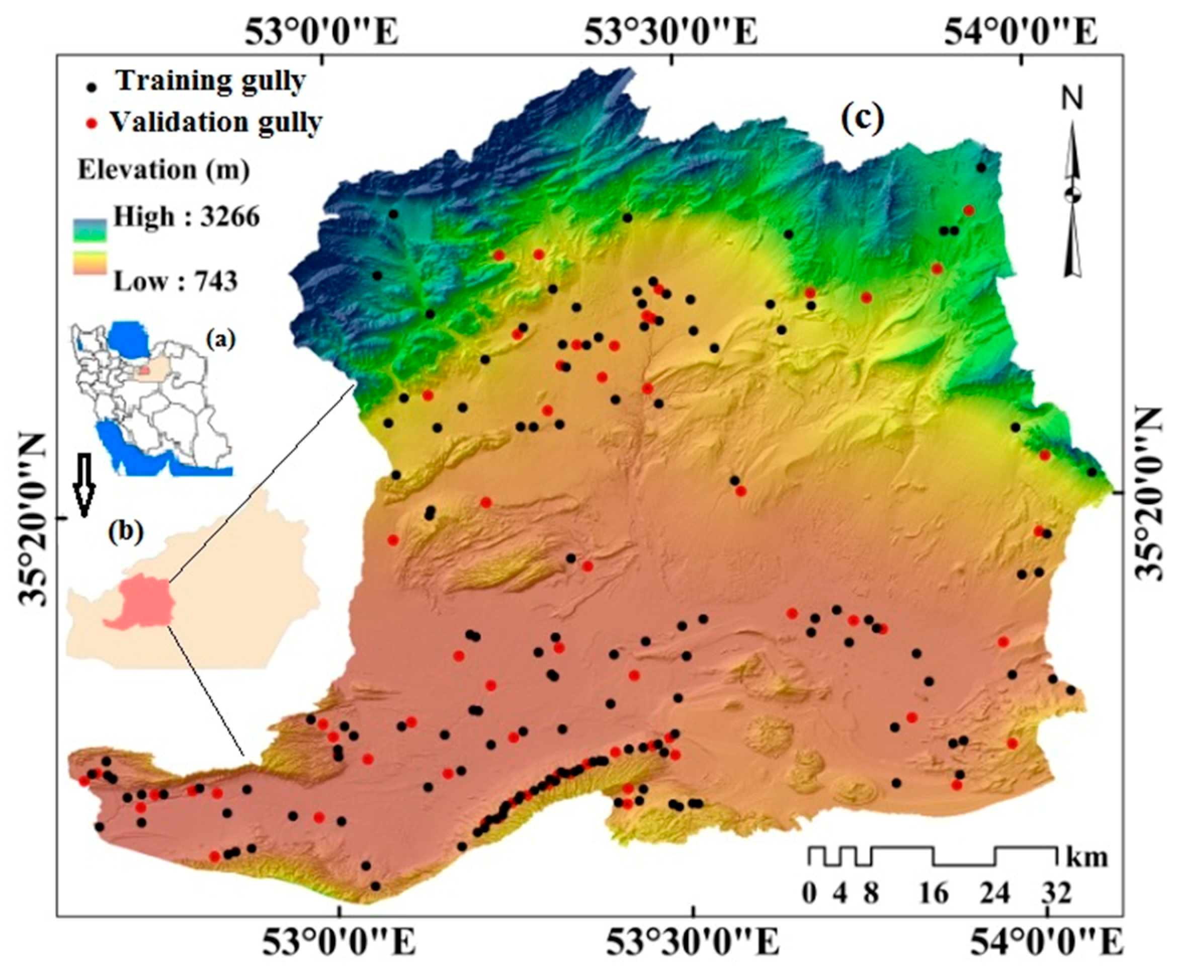
2.1. Study Area
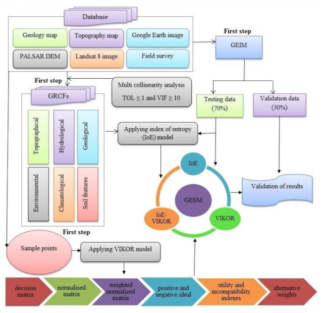
2.2. Methodology
2.3. Data Preparation
2.3.1. Gully Erosion Inventory Map
2.3.2. Gully-Related Conditioning Factors (GRCFs)
2.4. Multicollinearity Test (MT)
2.5. Models Used
2.5.1. Index of Entropy (IoE)
2.5.2. VIKOR
2.6. Model Validation
3. Results
3.1. Multicollinearity Test (MT)
3.2. Applying the Index of Entropy (IoE) Model
3.3. Applying the VIKOR Model
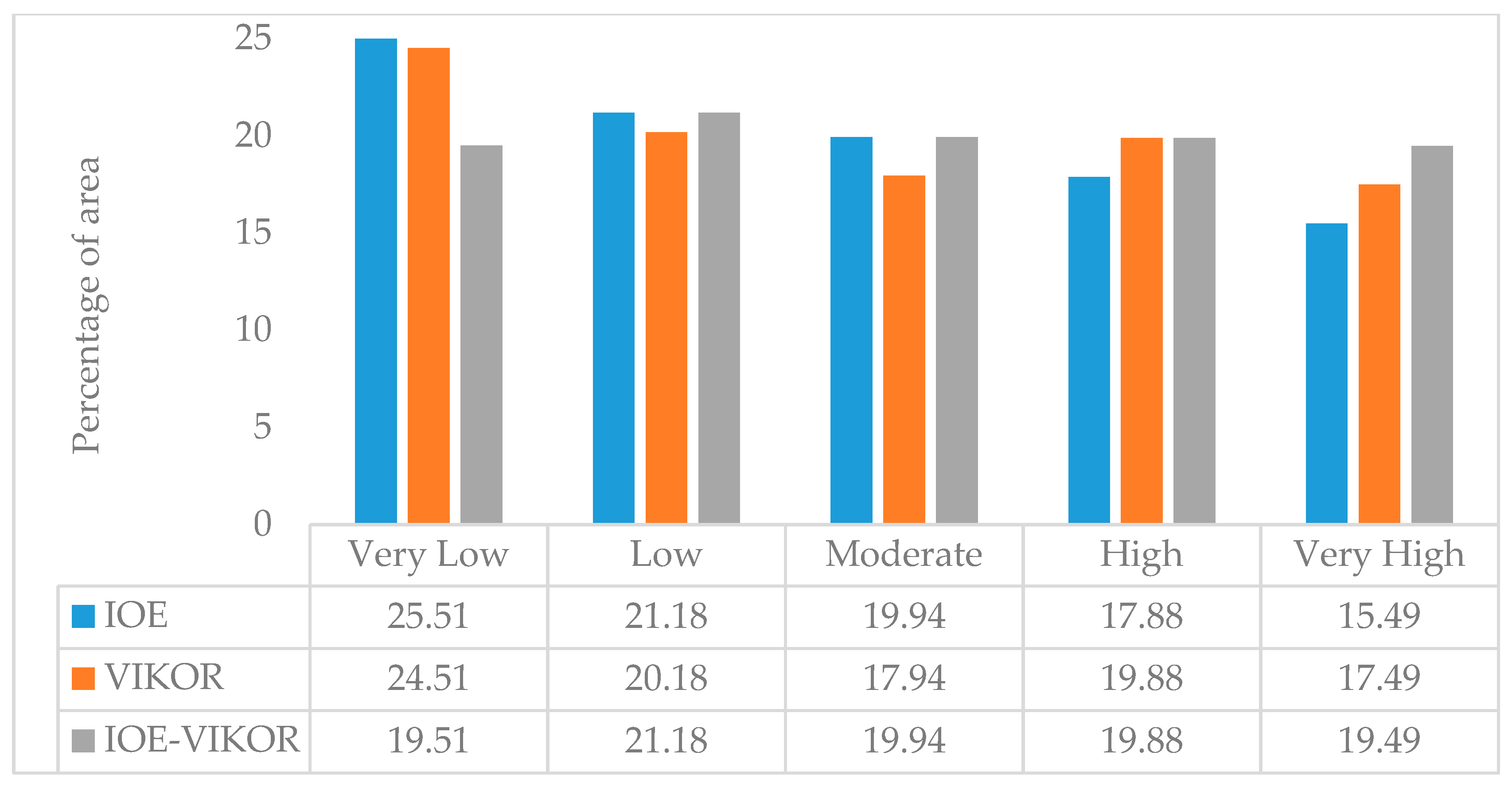
3.4. Integration of IoE and VIKOR Models and Validation
4. Discussion
5. Conclusions
Author Contributions
Funding
Acknowledgments
Conflicts of Interest
References
- Mekonnen, M.; Keesstra, S.D.; Baartman, J.E.; Stroosnijder, L.; Maroulis, J. Reducing sediment connectivity through man-made and natural sediment sinks in the Minizr Catchment, Northwest Ethiopia. Land Degrad. Dev. 2017, 28, 708–717. [Google Scholar] [CrossRef]
- Ben Slimane, A.; Raclot, D.; Evrard, O.; Sanaa, M.; Lefevre, I.; Le Bissonnais, Y. Relative contribution of rill/interrill and gully/channel erosion to small reservoir siltation in Mediterranean environments. Land Degrad. Dev. 2015, 27, 785–797. [Google Scholar] [CrossRef]
- Ayele, G.K.; Gessess, A.A.; Addisie, M.B.; Tilahun, S.A.; Tebebu, T.Y.; Tenessa, D.B.; Steenhuis, T.S. A biophysical and economic assessment of a community-based rehabilitated gully in the Ethiopian highlands. Land Degrad. Dev. 2016, 27, 270–280. [Google Scholar] [CrossRef]
- Castillo, C.; Marín-Moreno, V.J.; Pérez, R.; Muñoz-Salinas, R.; Taguas, E.V. Accurate automated assessment of gully cross-section geometry using the photogrammetric interface FreeXSapp. Earth Surf. Process. Landf. 2018, 43, 1726–1736. [Google Scholar] [CrossRef]
- Pulley, S.; Ellery, W.N.; Lagesse, J.V.; Schlegel, P.K.; Mcnamara, S.J. Gully erosion as a mechanism for wetland formation: An examination of two contrasting landscapes. Land Degrad. Dev. 2018, 29, 1756–1767. [Google Scholar] [CrossRef]
- Keesstra, S.; Mol, G.; de Leeuw, J.; Okx, J.; de Cleen, M.; Visser, S. Soil-related sustainable development goals: Four concepts to make land degradation neutrality and restoration work. Land 2018, 7, 133. [Google Scholar] [CrossRef]
- Hosseinalizadeh, M.; Kariminejad, N.; Rahmati, O.; Keesstra, S.; Alinejad, M.; Behbahani, A.M. How can statistical and artificial intelligence approaches predict piping erosion susceptibility? Sci. Total Environ. 2019, 646, 1554–1566. [Google Scholar] [CrossRef]
- Roscco, M.G.; Bull, L.G. Some factors controlling gully growth in fine grained sediment: A model applied in Southeast Spain. Catena 2000, 40, 127–146. [Google Scholar]
- Arabameri, A.; Pradhan, B.; Lombardo, L. Comparative assessment using boosted regression trees, binary logistic regression, frequency ratio and numerical risk factor for gully erosion susceptibility modelling. Catena 2019, 183, 104223. [Google Scholar] [CrossRef]
- Ireland, H.A.; Sharpe, C.F.; Eargle, D.H. Principles of Gully Erosion in the Piedmont of South Carolina; Technical Bulletin 633 USDA; United States Department of Agriculture: Washington, DC, USA, 1939.
- Brice, J.B. Erosion and deposition in loess-mantled Great Plains, Medecine Creek Drainage Basin, Nebraska. Geol. Surv. Prof. 1966, 235–339. [Google Scholar]
- Hauge, C. Soil erosion definitions. Calif. Geol. 1977, 30, 202–203. [Google Scholar]
- Imeson, A.C.; Kwaad, F.J.P.M. Gully types and Gully prediction. Geogr. Tijdschr. 1980, 14, 430–441. [Google Scholar]
- Poesen, J.; Vandaele, K.; Wesemael, B. Contribution of gully erosion to sediment production in cultivated lands and rangelands. Eros. Sediment. Yield Glob. Reg. Perspect. 1996, 236, 251–266. [Google Scholar]
- Heed, B.H. Morphology of gullies in the Colorado Rocky Mountains. Bull. Int. Assoc. Sci. Hydrol. 1970, 2, 79–89. [Google Scholar] [CrossRef]
- Morgan, R.P.C.; Mngomezulu, D. Threshold conditions for initiation of valley-side gullies in the Middle Veld of Swaziland. Catena 2003, 50, 401–414. [Google Scholar] [CrossRef]
- Zaimes, G.N.; Schultz, R.C. Assessing riparian conservation land management practice impacts on gully erosion in Iowa. Environ. Manag. 2012, 49, 1009–1021. [Google Scholar] [CrossRef] [PubMed]
- Valentin, C.; Poesen, J.; Li, Y. Gully erosion: Impacts, factors and control. Catena 2005, 63, 132–153. [Google Scholar] [CrossRef]
- Brooks, K.N.; Ffolliott, P.F.; Gregersen, H.M.; DeBano, L.F. Hydrology and the Management of Watersheds; Iowa State University Press: Ames, USA, 2003; p. 574. [Google Scholar]
- Arabameri, A.; Pradhan, B.; Pourghasemi, H.R.; Rezaei, K.; Kerle, N. Spatial modelling of gully erosion using GIS and R programing: A comparison among three data mining algorithms. Appl. Sci. 2018, 8, 1369. [Google Scholar] [CrossRef]
- Poesen, J.; Nachtergaele, J.; Verstraeten, G.; Valentin, C. Gully erosion and environment change: Importance and research needs. Catena 2003, 50, 91–133. [Google Scholar] [CrossRef]
- Deng, Q.; Qin, F.; Zhang, B.; Wang, H.; Luo, M.; Shu, C.; Liu, H.; Liu, G. Characterizing the morphology of gully cross-sections based on PCA: A case of Yuanmou Dry-Hot Valley. Geomorphology 2015, 228, 703–713. [Google Scholar] [CrossRef]
- Castillo, C.; Gómez, J.A. A century of gully erosion research: Urgency, complexity and study approaches. Earth Sci. Rev. 2016, 160, 300–319. [Google Scholar] [CrossRef]
- Qilin, Y.; Jiarong, G.; Yue, W.; Bintian, Q. Debris flow characteristics and risk degree assessment in Changyuan Gully, Huairou District, Beijing. Procedia Earth Planet. Sci. 2011, 2, 262–271. [Google Scholar]
- Moore, I.D.; Grayson, R.B.; Ladson, A.R. Digital terrain modelling: A review of hydrological, geomorphological, and biological applications. Hydrol. Process. 1991, 5, 3–30. [Google Scholar] [CrossRef]
- Vaezi, A.R.; Abbasi, M.; Keesstra, S.; Cerdà, A. Assessment of soil particle erodibility and sediment trapping using check dams in small semi-arid catchments. Catena 2017, 157, 227–240. [Google Scholar] [CrossRef] [Green Version]
- Zakerinejad, R.; Maerker, M. Prediction of gully erosion susceptibilities using detailed terrain analysis and maximum entropy modeling: A case study in the Mazayejan Plain, Southwest Iran. Geogr. Fis. E Din. Quat. 2014, 37, 67–76. [Google Scholar]
- Meliho, M.; Khattabi, A.; Mhammdi, N. A GIS-based approach for gully erosion susceptibility modelling using bivariate statistics methods in the Ourika watershed, Morocco. Environ. Earth Sci. 2018, 77, 655. [Google Scholar] [CrossRef]
- Rahmati, O.; Tahmasebipour, N.; Haghizadeh, A.; Pourghasemi, H.R.; Feizizadeh, B. Evaluating the influence of geo-environmental factors on gully erosion in a semi-arid region of Iran: An integrated framework. Sci. Total Environ. 2017, 579, 913–927. [Google Scholar] [CrossRef]
- Conforti, M.; Aucelli, P.P.; Robustelli, G.; Scarciglia, F. Geomorphology and GIS analysis formapping gully erosion susceptibility in the Turbolo streamcatchment (Northern Calabria, Italy). Nat. Hazards 2011, 56, 881–898. [Google Scholar] [CrossRef]
- Azareh, A.; Rahmati, O.; Rafiei-Sardooi, E.; Sankey, J.B.; Lee, S.; Shahabi, H.; BinAhmad, B. Modelling gully-erosion susceptibility in a semi-arid region, Iran: Investigation of applicability of certainty factor and maximum entropy models. Sci. Total Environ. 2019, 655, 684–696. [Google Scholar] [CrossRef]
- Zabihi, M.; Mirchooli, F.; Motevalli, A.; Darvishan, A.K.; Pourghasemi, H.R.; Zakeri, M.A.; Sadighi, F. Spatial modelling of gully erosion in Mazandaran Province, northern Iran. Catena 2018, 161, 1–13. [Google Scholar] [CrossRef]
- Conoscenti, C.; Angileri, S.; Cappadonia, C.; Rotigliano, E.; Agnesi, V.; Märker, M. Gully erosion susceptibility assessment by means of GIS-based logistic regression: A case of Sicily (Italy). Geomorphology 2014, 204, 399–411. [Google Scholar] [CrossRef] [Green Version]
- Dewitte, O.; Daoudi, M.; Bosco, C.; Eeckhaut, M. Predicting the susceptibility to gully initiation in data-poor regions. Geomorphology 2015, 228, 101–115. [Google Scholar] [CrossRef]
- Kornejady, A.; Heidari, K.; Nakhavali, M. Assessment of landslide susceptibility, semi-quantitative risk and management in the Ilam dam basin, Ilam. Iran. Environ. Resour. Res. 2015, 3, 85–109. [Google Scholar]
- Arabameri, A.; Pradhan, B.; Rezaei, K.; Yamani, M.; Pourghasemi, H.R.; Lombardo, L. Spatial modelling of gully erosion using Evidential Belief Function, Logistic Regression and a new ensemble EBF–LR algorithm. Land Degrad. Dev. 2018, 29, 4035–4049. [Google Scholar] [CrossRef]
- Dube, F.; Nhapi, I.; Murwira, A.; Gumindoga, W.; Goldin, J.; Mashauri, D.A. Potential of weight of evidence modelling for gully erosion hazard assessment in Mbire District—Zimbabwe. Phys. Chem. Earth 2014, 67, 145–152. [Google Scholar] [CrossRef]
- Pourghasemi, H.R.; Yousefi, S.; Kornejady, A.; Cerdà, A. Performance assessment of individual and ensemble data-mining techniques for gully erosion modeling. Sci. Total Environ. 2017, 609, 764–775. [Google Scholar] [CrossRef] [Green Version]
- Kornejady, A.; Ownegh, M.; Bahremand, A. Landslide susceptibility assessment using maximum entropy model with two different data sampling methods. Catena 2017, 152, 144–162. [Google Scholar] [CrossRef]
- Rahmati, O.; Tahmasebipour, N.; Haghizadeh, A.; Pourghasemi, H.R.; Feizizadeh, B. Evaluation of different machine learning models for predicting and mapping the susceptibility of gully erosion. Geomorphology 2017, 298, 118–137. [Google Scholar] [CrossRef]
- Arabameri, A.; Rezaei, K.; Pourghasemi, H.R.; Lee, S.; Yamani, M. GIS-based gully erosion susceptibility mapping: A comparison among three data-driven models and AHP knowledge-based technique. Environ. Earth Sci. 2018, 77, 628. [Google Scholar] [CrossRef]
- Conoscenti, C.; Agnesi, V.; Cama, M.; Alamaru Caraballo-Arias, N.; Rotigliano, E. Assessment of gully erosion susceptibility using multivariate adaptive regression splines and accounting for terrain connectivity. Land Degrad. Dev. 2018, 29, 724–736. [Google Scholar] [CrossRef]
- Arabameri, A.; Pradhan, B.; Rezaei, K. Gully erosion zonation mapping using integrated geographically weighted regression with certainty factor and random forest models in GIS. J. Environ. Manag. 2019, 232, 928–942. [Google Scholar] [CrossRef]
- Arabameri, A.; Pourghasemi, H.R. Spatial Modeling of Gully Erosion Using Linear and Quadratic Discriminant Analyses in GIS and R, 1st ed.; Pourghasemi, H.R., Gokceoglu, C., Eds.; Elsevier: Amsterdam, The Netherlands, 2019; p. 796. [Google Scholar]
- Hosseinalizadeh, M.; Kariminejad, N.; Chen, W.; Pourghasemi, H.R.; Alinejad, M.; Behbahani, A.M.; Tiefenbacher, J.P. Gully headcut susceptibility modeling using functional trees, naïve Bayes tree, and random forest models. Geoderma 2019, 342, 1–11. [Google Scholar] [CrossRef]
- Samani, A.N.; Rad, F.T.; Azarakhshi, M.; Rahdari, M.R.; Rodrigo-Comino, J.; Samani, A.N.; Rad, F.T.; Azarakhshi, M.; Rahdari, M.R.; Rodrigo-Comino, J. Assessment of the sustainability of the territories affected by gully head advancements through aerial photography and modeling estimations: A case study on Samal Watershed, Iran. Sustainability 2018, 10, 2909. [Google Scholar] [CrossRef]
- Keesstra, S.; Nunes, J.P.; Saco, P.; Parsons, T.; Poeppl, R.; Masselink, R.; Cerdà, A. The way forward: Can connectivity be useful to design better measuring and modelling schemes for water and sediment dynamics? Sci. Total Environ. 2018, 644, 1557–1572. [Google Scholar] [CrossRef]
- I.R. of Iran Meteorological Organization (IRIMO). Available online: http://www.mazan daranmet.ir. (accessed on 12 October 2017).
- Soil Survey Staff. Keys to Soil Taxonomy, 12th ed; USDA-Natural Resources Conservation Service: Washington, DC, USA, 2014.
- Geology Survey of Iran (GSI). Available online: http://www.gsi.ir/Main/Lang_en/index.html (accessed on 12 October 2017).
- Arabameri, A.; Pradhan, B.; Rezaei, K. Spatial prediction of gully erosion using ALOS PALSAR data and ensemble bivariate and data mining models. Geosci. J. 2019, 1–18. [Google Scholar] [CrossRef]
- Arabameri, A.; Cerda, A.; Tiefenbacher, J.P. Spatial pattern analysis and prediction of gully erosion using novel hybrid model of entropy-weight of evidence. Water 2019, 11, 1129. [Google Scholar] [CrossRef]
- Arabameri, A.; Pradhan, B.; Rezaei, K.; Conoscenti, C. Gully erosion susceptibility mapping using GIS-based multi-criteria decision analysis techniques. CATENA 2019, 180, 282–297. [Google Scholar] [CrossRef]
- Moore, I.D.; Burch, G.J.; Mackenzie, D.H. Topographic effects on the distribution of surface soil water and the location of ephemeral gullies. Am. Soc. Agric. Eng. 1988, 31, 1098–1107. [Google Scholar] [CrossRef]
- Yesilnacar, E.K. The application of computational intelligence to landslide susceptibility mapping in Turkey. Ph.D. Thesis, Department of Geomatics the University of Melbourne, Melbourne, Australia, March 2005. [Google Scholar]
- Yufeng, S.; Fengxiant, J. Landslide stability analysis based on generalized information entropy. Int. Conf. Environ. Sci. Inf. Appl. Technol. 2009, 83–85. [Google Scholar]
- Pourghasemi, H.R.; Mohammady, M.; Pradhan, B. Landslide susceptibility mapping using index of entropy and conditional probability models in GIS: Safarood Basin, Iran. Catena 2012, 97, 71–84. [Google Scholar] [CrossRef]
- Haghizadeh, A.; Siahkamari, S.; Haghiabi, A.H.; Rahamti, O. Forecasting flood-prone areas using Shannon’s entropy model. J. Earth Syst. Sci. 2017, 126, 39. [Google Scholar] [CrossRef]
- Arabameri, A.; Pourghasemi, H.R.; Cerda, A. Erodibility prioritization of sub-watersheds using morphometric parameters analysis and its mapping: A comparison among TOPSIS, VIKOR, SAW, and CF multi-criteria decision. Sci. Total Environ. 2018, 613, 1385–1400. [Google Scholar] [CrossRef] [PubMed]
- Arabameri, A. Application of the Analytic Hierarchy Process (AHP) for locating fire stations: Case study Maku City. Merit Res. J. ArtSoc. Sci. Humanit. 2014, 2, 1–10. [Google Scholar]
- Arabameri, A.; Rezaei, K.; Cerdà, A.; Conoscenti, C.; Kalantari, Z. A comparison of statistical methods and multi-criteria decision making to map flood hazard susceptibility in Northern Iran. Sci. Total Environ. 2019, 660, 443–458. [Google Scholar] [CrossRef]
- Arabameri, A.; Rezaei, K.; Cerda, A.; Lombardo, L.; Rodrigo-Comino, J. GIS-based groundwater potential mapping in Shahroud plain, Iran. A comparison among statistical (bivariate and multivariate), data mining and MCDM approaches. Sci. Total Environ. 2019, 658, 160–177. [Google Scholar] [CrossRef]
- Arabameri, A.; Pradhan, B.; Pourghasemi, H.R.; Rezaei, K. Identification of erosion-prone areas using different multi-criteria decision-making techniques and GIS. Geomat. Nat. Hazards Risk 2018, 9, 1129–1155. [Google Scholar] [CrossRef] [Green Version]
- Arabameri, A.; Ramesht, M.H. Site Selection of Landfill with emphasis on Hydrogeomorphological–environmental parameters Shahrood-Bastam watershed. Sci. J. Manag. Syst. 2017, 16, 55–80. [Google Scholar]
- Yamani, M.; Arabameri, A. Comparison and evaluation of three methods of multi attribute decision making methods in choosing the best plant species for environmental management (Case study: Chah Jam Erg). Nat. Environ. Chang. 2015, 1, 49–62. [Google Scholar]
- Arabameri, A. Zoning Mashhad Watershed for artificial recharge of underground aquifers using topsis model and GIS technique. Global J. Hum. Soc. Sci. B Geogr. Geo Sci. Environ. Disaster Manag. 2014, 14, 45–53. [Google Scholar]
- Chen, L.Y.; Wang, T.C. optimizing partners’choice in IS/IT outsourcing projects: The strategic decision of fuzzy VIKOR. Int. J. Prod. Econ. 2009, 120, 55–79. [Google Scholar] [CrossRef]
- Opricovic, S.; Tzeng, G. Extended VIKOR method in comparison with outranking methods. Eur. J. Oper. Res. 2006, 178, 514–529. [Google Scholar] [CrossRef]
- Romer, C.; Ferentinou, M. Shallow landslide susceptibility assessment in a semi-arid environment A Quaternary catchment of KwaZulu-Natal, South Africa. Eng. Geol. 2016, 201, 29–44. [Google Scholar] [CrossRef]
- Tien Bui, D.; Hoang, N.D.; Martínez-Álvarez, F.; Ngo, P.T.T.; Hoa, P.V.; Pham, T.D.; Samui, P.; Costache, R. A novel deep learning neural network approach for predicting flash flood susceptibility: A case study at a high frequency tropical storm area. Sci. Total Environ. 2019. [Google Scholar] [CrossRef]
- O’Brien, R.M. A caution regarding rules of thumb for variance inflation factors. Qual. Quant. 2007, 41, 673–690. [Google Scholar] [CrossRef]
- Rahmati, O.; Haghizadeh, A.; Pourghasemi, H.R.; Noormohamadi, F. Gully erosion susceptibility mapping: The role of GIS based bivariate statistical models and their comparison. Nat. Hazards 2016, 82, 1231–1258. [Google Scholar] [CrossRef]
- Arabameri, A.; Yamani, M.; Pradhan, B.; Melesse, A.; Shirani, K.; Tien Bui, D. Novel ensembles of COPRAS multi-criteria decision-making with logistic regression, boosted regression tree, and random forest for spatial prediction of gully erosion susceptibility. Sci. Total Environ. 2019, 688, 903–916. [Google Scholar] [CrossRef]
- Mohammadkhan, S.; Ahmadi, H.; Jafari, M. Relationship between soil erosion, slope, parent material, and distance to road (Case study: Latian Watershed, Iran). Arab. J. Geosci. 2011, 4, 331–338. [Google Scholar] [CrossRef]
- Nazari Samani, A.; Khosravi, H.; Mesbahzadeh, T.; Azarakhshi, M.; Rahdari, M.R. Determination of sand dune characteristics through geomorphometry and wind data analysis in central Iran (Kashan Erg). Arab. J. Geosci. 2016, 9, 716. [Google Scholar] [CrossRef]
- Cerdà, A. Soil water erosion on road embankments in eastern Spain. Sci. Total Environ. 2007, 378, 151–155. [Google Scholar] [CrossRef]
- Yousefi, S.; Sadeghi, S.H.; Mirzaee, S.; Ploeg, M.; Keesstra, S.; Cerdà, A. Spatio-temporal variation of throughfall in a hyrcanian plain forest stand in Northern Iran. J. Hydrol. Hydromech. 2018, 66, 97–106. [Google Scholar] [CrossRef]
- García-Ruiz, J.; Lasanta, T.; Alberto, F. Soil erosion by piping in irrigated fields. Geomorphology 1997, 20, 269–278. [Google Scholar] [CrossRef]
- Romero Díaz, A.; Marín Sanleandro, P.; Sánchez Soriano, A.; Belmonte Serrato, F.; Faulkner, H. The causes of piping in a set of abandoned agricultural terraces in southeast Spain. Catena 2007, 69, 282–293. [Google Scholar] [CrossRef]
- Bravo-Espinosa, M.; Mendoza, M.E.; Carlón Allende, T.; Medina, L.; Sáenz-Reyes, J.T.; Páez, R. Effects of converting forest to avocado orchards on topsoil properties in the trans-Mexican volcanic system, Mexico. Land Degrad. Dev. 2014, 25, 452–467. [Google Scholar] [CrossRef]
- Ben Slimane, A.; Raclot, D.; Rebai, H.; Le Bissonnais, Y.; Planchon, O.; Bouksila, F. Combining field monitoring and aerial imagery to evaluate the role of gully erosion in a Mediterranean catchment (Tunisia). Catena 2018, 170, 73–83. [Google Scholar] [CrossRef]
- Yitbarek, T.W.; Belliethathan, S.; Stringer, L.C. The onsite cost of gully erosion and cost-benefit of gully rehabilitation: A case study in Ethiopia. Land Degrad. Dev. 2012, 23, 157–166. [Google Scholar] [CrossRef]
- Ramakrishna, D.; Ghose, M.K.; Vinu Chandra, R.; Jeyaram, A. Probabilistic techniques, GIS and remote sensing in landslide hazard mitigation: A case study from Sikkim Himalayas, India. Geocarto Int. 2005, 20, 53–58. [Google Scholar] [CrossRef]
- Sharma, L.P.; Patel, N.; Ghose, M.K.; Debnath, P. Influence of Shannon’s entropy on lands lide—Causing parameters for vulnerability study and zonation-a case study in Sikkim, India. Arab. J. Geosci. 2010, 5, 421–431. [Google Scholar] [CrossRef]


| Factor | Source | Resolution | Classes | Method |
|---|---|---|---|---|
| Elevation | PALSAR DEM | 12.5 m | 1. (< 890 m), 2. (890 m–935 m), 3. (935 m–1100 m), 4. (1100 m–1600 m), 5. (>1600 m) | Natural break |
| Slope | PALSAR DEM | 12.5 m | 1. (<5°), 2. (5°–10°), 3. (10°–20°), 4. (20°–30°), 5. (>30°) | Natural break |
| Aspect | PALSAR DEM | 12.5 m | 1. Flat (–1°), 2. North (337.5–360°, 0–22.5°), 3. Northeast (22.5–67.5°), 4. East (67.5–112.5°), 5. Southeast (112.5–157.5°), 6. South (157.5–202.5°), 7. Southwest (202.5–247.5°), 8. West (247.4–292.5°), and 9. Northwest (292.5–337.5°) | Equal interval |
| Plan curvature | PALSAR DEM | 12.5 m | 1. Concave (<–0.05), 2. Flat (–0.05–0.05), 3. Convex (>0.5) | Natural break |
| SPI | PALSAR DEM | 12.5 m | 1. (<9.2), 2. (9.2–11.03), 3. (11.03–3.02). 4. (13.02–15.89). 5. (>15.89) | Natural break |
| TWI | PALSAR DEM | 12.5 m | 1. (<4.41), 2. (4.41–6.84), 3. (6.84–10.44) (>10.44) | Natural break |
| Rainfall | weather stations | .... | 1. (<–1.06), 2. (–1.06–0.87), 3. (0.87–3.99), 4. (>3.99) | Natural break |
| Soil type | Soil map | 1:100,000 | 1. (<125 mm), 2. (125–215 mm), 3. (215–350 mm), 4. (>350 mm) | Natural break |
| Drainage density | PALSAR DEM | 12.5 m | 1. (<0.14 km/km2), 2. (0.14–0.18 km/km2), 3. (0.18–0.31 km/km2), 4 (>0.31 km/km2) | Natural break |
| Distance to river | PALSAR DEM | 12.5 m | 1. (<650 m), 2. (650 m–870 m), 3. (870 m–1500 m), 4. (1500 m–3500 m), 5. (>3500 m) | Natural break |
| Distance to road | Topography map | 1:50,000 | 1. (<1700 m), 2. (1700–5000 m), 3. (5000–10,000 m), 4. (10,000–23,000 m), 5. (>23,000) | Natural break |
| Distance to fault | Geology map | 1:100,000 | 1. (<5000 m), 2 (5000–10,000 m), 3. (10,000–17,000), 4. (>17,000) | Natural break |
| Lithology | Geology map | 1:100,000 | 1. (A), 2.(B), 3. (C), 4. (D), 5. (E), 6. (F), 7. (J), 8. (H). | Lithological units |
| LU/LC | Landuse map | 1:100,000 | 1. (Agriculture), 2. (Orchard), 3. (Barelans), 4. (Kavir), 5. (Modrange), 6. (Poorrange), 7. (Rock), 8. (Urban), 9. (Water), 10. (Woodland). | Supervised classification |
| NDVI | Landsat 8 | 30 m | 1. (< - 0.15), 2. (- 0.15 – 0.17), 3 (> 0.17) | Natural break |
| Factors | Collinearity Statistics | |
|---|---|---|
| Tolerance | VIF | |
| (Constant) | - | - |
| Aspect | 0.890 | 1.124 |
| Convergence | 0.0791 | 11.264 |
| Total curvature | 0.067 | 14.980 |
| Elevation | 0.106 | 4.012 |
| Drainage density | 0.481 | 2.080 |
| Dis to fault | 0.629 | 1.590 |
| Dis to river | 0.549 | 1.822 |
| Dis to road | 0.620 | 1.613 |
| Profile curvature | 0.0132 | 17.604 |
| Plan curvature | 0.179 | 4.598 |
| NDVI | 0.350 | 2.860 |
| LS | 0.0808 | 11.238 |
| TWI | 0.671 | 1.490 |
| SPI | 0.721 | 1.386 |
| Slope | 0.467 | 2.141 |
| Rainfall | 0.331 | 3.020 |
| LU | 0.564 | 1.775 |
| Soil type | 0.283 | 3.535 |
| Lithology | 0.867 | 1.153 |
| Factor | Class | Domain Pixels | GULLY PIXELS | Pij | Wj | ||
|---|---|---|---|---|---|---|---|
| No | % | No | % | ||||
| Elevation (m) | <890 | 2,879,578 | 29.89 | 60 | 37.04 | 1.24 | 0.05 |
| 890–935 | 710,494 | 7.37 | 17 | 10.49 | 1.42 | ||
| 935–1100 | 2,013,677 | 20.90 | 37 | 22.84 | 1.09 | ||
| 1100–1600 | 2,313,076 | 24.01 | 39 | 24.07 | 1.00 | ||
| >1600 | 1,717,478 | 17.83 | 9 | 5.56 | 0.31 | ||
| Slope (°) | <5 | 6,899,986 | 71.62 | 116 | 71.60 | 1.00 | 0.24 |
| 5–10 | 1,070,376 | 11.11 | 28 | 17.28 | 1.56 | ||
| 10–20 | 924,930 | 9.60 | 18 | 11.11 | 1.16 | ||
| 20–30 | 481,844 | 5.00 | 0 | 0.00 | 0.00 | ||
| >30 | 257,167 | 2.67 | 0 | 0.00 | 0.00 | ||
| Aspect | F | 566,040 | 5.88 | 4 | 2.47 | 0.42 | 0.02 |
| N | 961,571 | 9.99 | 18 | 11.11 | 1.11 | ||
| NE | 710,471 | 7.38 | 17 | 10.49 | 1.42 | ||
| E | 872,929 | 9.07 | 23 | 14.20 | 1.57 | ||
| SE | 1,383,590 | 14.38 | 31 | 19.14 | 1.33 | ||
| S | 1,791,970 | 18.62 | 23 | 14.20 | 0.76 | ||
| SW | 1,428,212 | 14.84 | 18 | 11.11 | 0.75 | ||
| W | 994,513 | 10.33 | 11 | 6.79 | 0.66 | ||
| NW | 915,376 | 9.51 | 17 | 10.49 | 1.10 | ||
| Curvature (100/m) | concave | 325,238 | 3.38 | 9 | 5.56 | 1.65 | 0.41 |
| flat | 8,726,972 | 90.58 | 144 | 88.89 | 0.98 | ||
| convex | 582,093 | 6.04 | 9 | 5.56 | 0.92 | ||
| SPI (100/m) | <9.2 | 3,016,197 | 31.36 | 64 | 39.51 | 1.26 | 0.53 |
| 9.2–11.03 | 2,592,536 | 26.95 | 25 | 15.43 | 0.57 | ||
| 11.03–13.02 | 2,452,601 | 25.50 | 26 | 16.05 | 0.63 | ||
| 13.02–15.89 | 1,213,412 | 12.61 | 14 | 8.64 | 0.69 | ||
| >15.89 | 344,608 | 3.58 | 33 | 20.37 | 0.69 | ||
| TWI (100/m) | < 4.41 | 2,642,289 | 27.47 | 40 | 24.69 | 0.90 | 0.41 |
| 4.41–6.84 | 4,350,350 | 45.22 | 60 | 37.04 | 0.82 | ||
| 6.84–10.44 | 2,077,423 | 21.60 | 27 | 16.67 | 0.77 | ||
| >10.44 | 549,292 | 5.71 | 35 | 21.60 | 3.78 | ||
| Rainfall (mm) | <125 | 6,422,553 | 66.64 | 118 | 72.84 | 1.09 | 0.11 |
| 125–215 | 1,961,321 | 20.35 | 39 | 24.07 | 1.18 | ||
| 215–350 | 894,195 | 9.28 | 4 | 2.47 | 0.27 | ||
| >350 | 358,963 | 3.72 | 1 | 0.62 | 0.17 | ||
| Soil type | Rock Outcrops/Entisols | 2,878,863 | 29.87 | 27 | 16.67 | 0.56 | 1.8 |
| Entisols/Aridisols | 1,495,535 | 15.52 | 18 | 11.11 | 0.72 | ||
| Inceptisols | 63,063 | 0.65 | 17 | 10.49 | 16 | ||
| Aridisols | 842,361 | 8.74 | 58 | 35.80 | 4.10 | ||
| Bad Lands | 2,307,771 | 23.95 | 42 | 25.93 | 1.08 | ||
| Salt Flats | 2,049,443 | 21.27 | 0 | 0.00 | 0.00 | 0.03 | |
| Drainage density (km/km2) | <0.14 | 2,847,934 | 29.64 | 51 | 31.48 | 1.06 | |
| 0.14–0.18 | 1,233,569 | 12.84 | 23 | 14.20 | 1.11 | ||
| 0.18–0.31 | 3,165,207 | 32.95 | 44 | 27.16 | 0.82 | ||
| >0.31 | 2,360,559 | 24.57 | 44 | 27.16 | 1.11 | ||
| Distance to river (m) | <650 | 2,715,295 | 28.19 | 75 | 46.30 | 1.64 | 0.049 |
| 650–870 | 793,728 | 8.24 | 12 | 7.41 | 0.90 | ||
| 870–1500 | 1,906,357 | 19.79 | 23 | 14.20 | 0.72 | ||
| 1500–3500 | 3,202,074 | 33.24 | 29 | 17.90 | 0.54 | ||
| >3500 | 1,016,201 | 10.55 | 23 | 14.20 | 1.35 | ||
| Distance to fault (m) | <5000 | 3,642,736 | 37.90 | 85 | 52.80 | 1.39 | 0.001 |
| 5000–10,000 | 2,778,443 | 28.91 | 30 | 18.63 | 0.64 | ||
| 10,000–17,000 | 2,095,468 | 21.80 | 34 | 21.12 | 0.97 | ||
| >17,000 | 1,094,885 | 11.39 | 12 | 7.45 | 0.65 | ||
| Distance to road (m) | <1700 | 1,705,351 | 17.74 | 30 | 18.52 | 1.04 | 0.02 |
| 1700–5000 | 2,582,564 | 26.86 | 36 | 22.22 | 0.83 | ||
| 5000–10,000 | 2,308,778 | 24.02 | 28 | 17.28 | 0.72 | ||
| 10,000–23,000 | 1,840,552 | 19.15 | 39 | 24.07 | 1.26 | ||
| >23,000 | 1,176,036 | 12.23 | 29 | 17.90 | 1.46 | ||
| Lithology | Marl, Gypsum | 2,738,777 | 28.42 | 63 | 38.89 | 1.37 | 0.048 |
| Conglomerate, Sandstone, Shale, Tuff | 803,953 | 8.34 | 6 | 3.70 | 0.44 | ||
| Terraces deposits | 3,718,139 | 38.58 | 45 | 27.78 | 0.72 | ||
| Dolomite, Limestone, Sandstone, Shale | 653,507 | 6.78 | 9 | 5.56 | 0.82 | ||
| Fluvial conglomerate | 288,376 | 2.99 | 3 | 1.85 | 0.62 | ||
| Volcanic rocks | 378,802 | 3.93 | 11 | 6.79 | 1.73 | ||
| Clay | 817,583 | 8.48 | 22 | 13.58 | 1.60 | ||
| Salt | 237,994 | 2.47 | 3 | 1.85 | 0.75 | ||
| LU/LC | Agriculture | 175,440 | 1.83 | 4 | 2.47 | 1.35 | 1.3 |
| Orchard | 6315 | 0.07 | 0 | 1.23 | 0 | ||
| Bareland | 896,113 | 9.33 | 9 | 5.56 | 0.60 | ||
| Kavir | 3,025,781 | 31.49 | 83 | 51.23 | 1.63 | ||
| Modrange | 984,453 | 10.24 | 4 | 2.47 | 0.24 | ||
| Poorrange | 3,230,325 | 33.62 | 44 | 27.16 | 0.81 | ||
| Rock | 1,145,924 | 11.92 | 14 | 8.64 | 0.72 | ||
| Urban | 81,661 | 0.85 | 0 | 1.23 | 0 | ||
| Water | 185 | 0.00 | 0 | 0.00 | 0 | ||
| Woodland | 63,487 | 0.66 | 0 | 0.00 | 0 | ||
| NDVI | <–0.15 | 5,656,113 | 58.77 | 100 | 61.73 | 1.05 | 0.24 |
| –0.15–0.17 | 3,953,406 | 41.08 | 62 | 38.27 | 0.93 | ||
| >0.17 | 14,906 | 0.15 | 0 | 0.00 | 0.00 | ||
| pint | VIKOR-IoE | VIKOR | ||||
|---|---|---|---|---|---|---|
| S | R | Q | S | R | Q | |
| 1 | 2.088 | 1.418 | 0.095 | 0.732 | 0.326 | 0.117 |
| 2 | 0.108 | 0.022 | 0.989 | 0.065 | 0.015 | 0.983 |
| 3 | 1.808 | 1.420 | 0.158 | 0.552 | 0.327 | 0.231 |
| 4 | 1.295 | 1.021 | 0.401 | 0.399 | 0.235 | 0.459 |
| 5 | 0.276 | 0.193 | 0.897 | 0.166 | 0.118 | 0.773 |
| 6 | 0.412 | 0.193 | 0.866 | 0.238 | 0.118 | 0.727 |
| 7 | 2.077 | 1.418 | 0.097 | 0.724 | 0.326 | 0.122 |
| 8 | 1.791 | 1.420 | 0.162 | 0.540 | 0.327 | 0.239 |
| 9 | 0.416 | 0.193 | 0.865 | 0.249 | 0.118 | 0.720 |
| 10 | 1.648 | 1.110 | 0.293 | 0.588 | 0.255 | 0.309 |
| 11 | 2.072 | 1.418 | 0.098 | 0.724 | 0.326 | 0.122 |
| 12 | 0.134 | 0.073 | 0.967 | 0.091 | 0.037 | 0.935 |
| 13 | 0.126 | 0.028 | 0.983 | 0.067 | 0.015 | 0.981 |
| 14 | 0.090 | 0.033 | 0.990 | 0.065 | 0.020 | 0.976 |
| 15 | 1.800 | 1.418 | 0.161 | 0.550 | 0.326 | 0.233 |
| 16 | 1.480 | 1.110 | 0.331 | 0.455 | 0.255 | 0.394 |
| 17 | 1.773 | 1.420 | 0.166 | 0.537 | 0.327 | 0.241 |
| 18 | 1.836 | 1.420 | 0.152 | 0.573 | 0.327 | 0.218 |
| 19 | 1.523 | 1.110 | 0.321 | 0.491 | 0.255 | 0.371 |
| 20 | 0.103 | 0.025 | 0.989 | 0.060 | 0.017 | 0.984 |
| 21 | 1.360 | 1.021 | 0.387 | 0.441 | 0.235 | 0.432 |
| 22 | 1.380 | 1.021 | 0.382 | 0.442 | 0.235 | 0.431 |
| 23 | 0.590 | 0.335 | 0.780 | 0.343 | 0.206 | 0.536 |
| 24 | 0.231 | 0.134 | 0.926 | 0.120 | 0.068 | 0.873 |
| 25 | 1.170 | 1.021 | 0.430 | 0.324 | 0.235 | 0.506 |
| 26 | 0.423 | 0.193 | 0.863 | 0.243 | 0.118 | 0.723 |
| 27 | 0.195 | 0.097 | 0.945 | 0.122 | 0.060 | 0.884 |
| 28 | 0.437 | 0.338 | 0.814 | 0.276 | 0.208 | 0.576 |
| 29 | 2.027 | 1.418 | 0.109 | 0.684 | 0.326 | 0.148 |
| 30 | 1.125 | 1.021 | 0.440 | 0.299 | 0.235 | 0.522 |
| 31 | 0.421 | 0.193 | 0.864 | 0.249 | 0.118 | 0.720 |
| 32 | 1.478 | 1.110 | 0.332 | 0.475 | 0.255 | 0.381 |
| 33 | 0.102 | 0.026 | 0.989 | 0.067 | 0.016 | 0.981 |
| 34 | 1.792 | 1.418 | 0.162 | 0.538 | 0.326 | 0.241 |
| 35 | 1.930 | 1.418 | 0.131 | 0.618 | 0.326 | 0.190 |
| 36 | 1.798 | 1.420 | 0.160 | 0.541 | 0.327 | 0.238 |
| 37 | 1.848 | 1.418 | 0.149 | 0.580 | 0.326 | 0.214 |
© 2019 by the authors. Licensee MDPI, Basel, Switzerland. This article is an open access article distributed under the terms and conditions of the Creative Commons Attribution (CC BY) license (http://creativecommons.org/licenses/by/4.0/).
Share and Cite
Arabameri, A.; Cerda, A.; Rodrigo-Comino, J.; Pradhan, B.; Sohrabi, M.; Blaschke, T.; Tien Bui, D. Proposing a Novel Predictive Technique for Gully Erosion Susceptibility Mapping in Arid and Semi-arid Regions (Iran). Remote Sens. 2019, 11, 2577. https://doi.org/10.3390/rs11212577
Arabameri A, Cerda A, Rodrigo-Comino J, Pradhan B, Sohrabi M, Blaschke T, Tien Bui D. Proposing a Novel Predictive Technique for Gully Erosion Susceptibility Mapping in Arid and Semi-arid Regions (Iran). Remote Sensing. 2019; 11(21):2577. https://doi.org/10.3390/rs11212577
Chicago/Turabian StyleArabameri, Alireza, Artemi Cerda, Jesús Rodrigo-Comino, Biswajeet Pradhan, Masoud Sohrabi, Thomas Blaschke, and Dieu Tien Bui. 2019. "Proposing a Novel Predictive Technique for Gully Erosion Susceptibility Mapping in Arid and Semi-arid Regions (Iran)" Remote Sensing 11, no. 21: 2577. https://doi.org/10.3390/rs11212577