A Two-Stage Fusion Framework to Generate a Spatio–Temporally Continuous MODIS NDSI Product over the Tibetan Plateau

Abstract

The Tibetan Plateau (TP) is an important component of the global environmental system, on which the snow cover greatly affects the regional climate and ecology. Moderate resolution imaging spectroradiometer (MODIS) snow cover products have been demonstrated to be appropriate for investigating the snow cover over the TP. However, they are subject to cloud obscuration, and the TP’s extremely complex terrain makes the snow monitoring difficult. Therefore, in this paper, we propose a two-stage spatio–temporal fusion framework for the cloud removal of MODIS C6 snow products, including an adjusted Terra and Aqua combination (TAC) and a spatio–temporal fusion based on Gaussian kernel function and error correction (STF-GKF-EC). To the best of our knowledge, this is the first time that a spatio–temporally continuous daily 500-m MODIS normalized difference snow index (NDSI) product has been generated for the TP, which greatly improves the spatial and temporal resolutions of the current snow cover products. The main stage, STF-GKF-EC, adaptively weights the spatial and temporal correlations by the Gaussian kernel function, and further takes the rapid changes of snow cover into consideration through the error correction. The experiments indicated that STF-GKF-EC removes clouds completely, achieving an overall accuracy (OA) and mean absolute error (MAE) of 91.48% and 3.88, respectively. Based on the cloud-removed results, during 2001–2017, as far as the intra-annual variation is concerned, a large proportion of the snow cover appears between October and May, with a peak in February/March, and the variation is mainly controlled by temperature. For the inter-annual variation, an obvious increasing trend of 0.68/year for NDSI is observed before 2005, followed by a slight decreasing trend of 0.16/year, in which precipitation is a better explanation factor than temperature.

1. Introduction

As the “third pole of the planet”, the Tibetan Plateau (TP) has a considerable impact on regional climate and ecology. With global warming in recent decades, the TP is undergoing glacier retreat, abnormal snow cover change, permafrost degradation, and weakening of the ecosystem [1]. Snow is a significant and sensitive element of the climate system, affecting the surface energy balance [2] and hydrological circulation [3,4]. For example, when the snow melts early, the peak of river runoff will shift from summer and autumn, when water demand is highest, to winter and spring, when water demand is lower [5], which will seriously affect the development of agriculture and the supply of municipal water in the downstream areas. Given these facts, it is essential to monitor the snow cover variability over the TP.

Compared with meteorological station data that are distributed sparsely and unevenly, satellite-based remote sensing data are notably more effective in describing the spatio–temporal patterns of snow cover at a large scale. Satellite-based snow products include microwave-based and optical-based products. Microwave-based snow products derived from active [6] or passive sensors [7,8,9] provide the snow depth (SD) or snow water equivalent (SWE) data with a long time series. However, the active microwave sensors only recognize wet snow [10], and the passive microwave-based products are reliable under dry conditions, but their spatial resolutions are too low to describe detailed information. In contrast, optical-based sensors [11,12,13] can acquire snow cover data with more appropriate spatial and temporal resolutions, taking advantage of the distinct reflection characteristics of snow in the visible and shortwave infrared bands. Therefore, optical snow products are widely applied in hydrological research, among which the moderate resolution imaging spectroradiometer (MODIS) snow products are particularly popular [14]. Nevertheless, heavy cloud contamination severely limits the application of the MODIS products [15,16]. As a result, there has been a lot of research on cloud removal to generate spatio–temporally seamless MODIS snow cover products.

Firstly, from a methodological perspective, the algorithms for removing the clouds of MODIS snow products can be mainly classified as temporal filtering methods, spatial filtering methods, multi-source fusion methods, and spatio–temporal union methods. Temporal filtering methods, e.g., the Terra and Aqua combination (TAC) [17], multi-day combination (MDC) [18,19], and seasonal filtering [20], assign each cloud pixel an appropriate value based on the pixels within a given time window. However, temporally continuous cloud cover and rapid snow cover changes can seriously reduce the accuracy. Spatial filtering methods, including the snow-line method (SNOWL) [21], neighborhood filtering (NF) [22], and function-based spatial interpolation [23], estimate the cloudy pixels according to the spatially selected non-cloud pixels. However, when confronted with high cloud cover, spatial filtering usually cannot obtain a satisfactory cloud removal effect. These two types of methods are applied to the same kind of snow cover data, so their complementarity is limited. Therefore, much attention has been paid to multi-source fusion methods [24,25,26,27,28,29,30], where optical observations are blended with microwave observations and/or meteorological station observations. It has been demonstrated that the multi-source fusion methods can completely remove the clouds, but the accuracy relies on the complementarity and accuracy of the input data [14]. These methods perform well in binary snow cover mapping, but are likely to lose details due to the great differences in characteristics and spatial resolution between the different types of products. A better practice for producing cloud-free snow cover products is to integrate the spatial and temporal information of optical-based products. Their union can remove clouds completely, with a higher accuracy than temporal filtering and spatial filtering [31,32]. For example, Gafurov and Bárdossy [18] proposed a six-step spatio–temporal union algorithm to remove clouds gradually; Gascoin et al. [33] combined the TAC, NF, MDC and a classification tree to fill the cloud-covered gaps; Dariane et al. [34] developed a four-step approach of the TAC, MDC, SNOWL, and NF with elevation constraints; and Li et al. [35] developed an adaptive spatio–temporal weighted method to integrate the spatial and temporal information adaptively. Nevertheless, the existing spatio–temporal union methods have difficulty in restoring cloud-contaminated snow cover with rapid changes, especially on the TP, with inconsistent regional changes.

From the perspective of the product category, the previous research on cloud-free MODIS snow product generation has primarily concentrated on collection 5 (C5) and collection 6 (C6). C5 provides the binary snow cover area (SCA) and fractional snow cover (FSC) data. The above algorithms are classically aimed at the SCA products of MODIS C5. However, after the MODIS C6 snow cover products were published in 2016, the previous SCA was replaced by the normalized difference snow index (NDSI), and the FSC was not provided. Since the NDSI is a more accurate description of snow presence, as a result of its consideration of the high reflectance of visible bands and the low reflectance of shortwave infrared bands in snow-covered areas [36], the focus has gradually moved to the MODIS NDSI products. Crawford demonstrated that the MODIS Terra C6 FSC has a good consistency with Landsat TM/ETM+ FSC [37]. Given the different selections of NDSI threshold, Zhang et al. evaluated the C6 products across China [38]. For cloud removal, some studies have first converted the NDSI to SCA or FSC, and then removed the clouds, as in the C5 products [39,40,41]. In addition, using eight-day MOD10C2 data, Li et al. [42] confirmed that the snow cover patterns on the TP exhibit significant spatio–temporal heterogeneity, and that the snow cover fraction decreased slightly by ~1.1% from 2001 to 2014. In general, for the snow cover variability over the TP, the current research based on NDSI products is still scarce and the spatial and temporal resolutions are coarse.

As a result, in this paper, we propose a novel two-stage spatio–temporal fusion framework to generate a cloud-free MODIS NDSI product, and we further investigate the snow cover variability over the TP at higher spatial and temporal resolutions than previous studies. First, a framework integrating an adjusted Terra and Aqua combination (TAC) and a spatio–temporal fusion based on Gaussian kernel function and error correction (STF-GKF-EC) is introduced. The main stage, STF-GKF-EC, integrates the spatial and temporal information based on a unified spatio–temporal weight, and greatly mitigates the effects of rapid snow cover changes through the error correction. Then, the cloud removal effect and accuracy of this method are tested in the simulated experiment. Finally, the method is applied to generate the daily cloud-free NDSI product with a spatial resolution of 500 m over the TP during 2001–2017, which is used to analyze the intra-annual and inter-annual variabilities of snow cover and their response to temperature and precipitation.

2. Study Area and Data

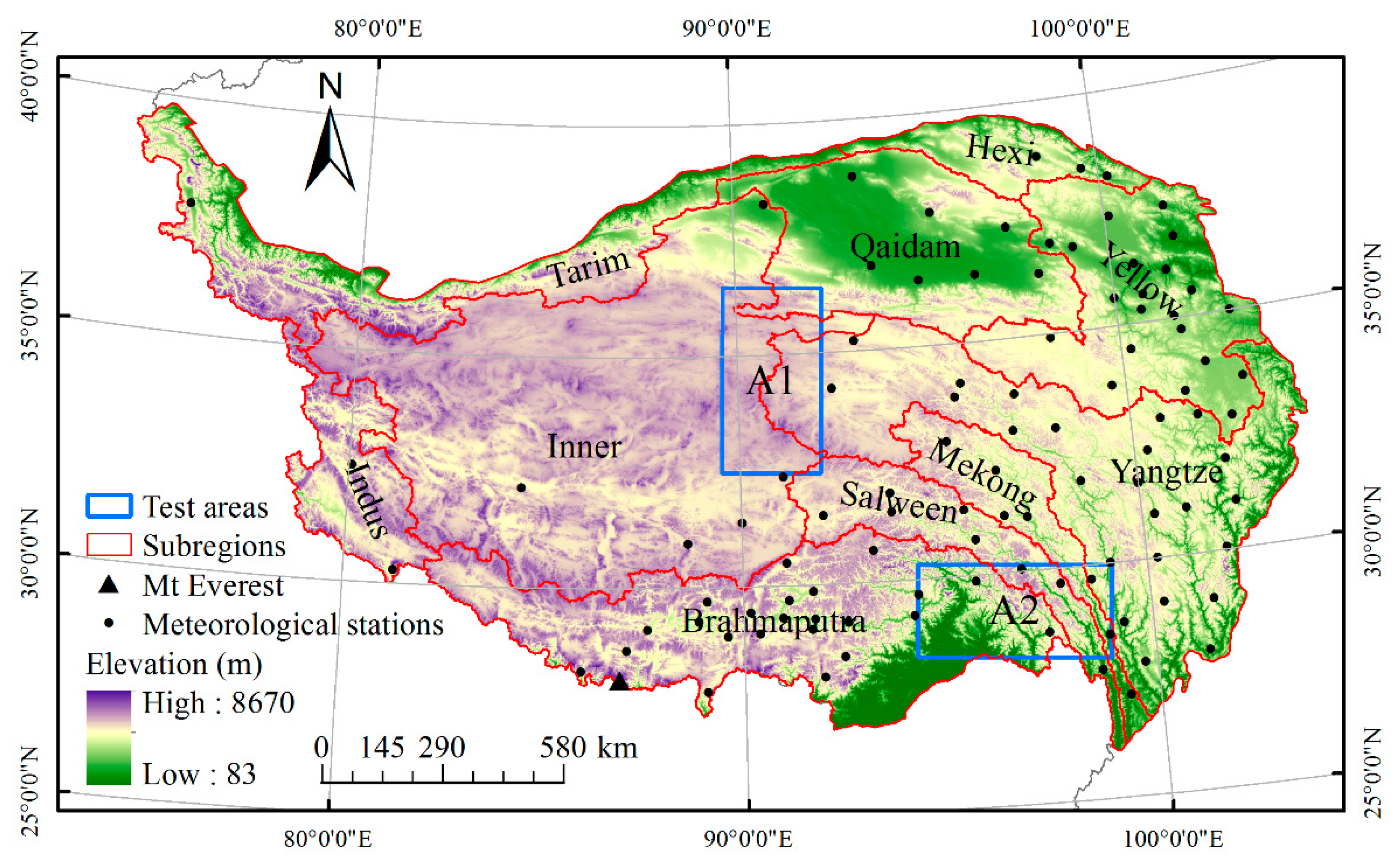
2.1. Study Area

The TP is located in central Eurasia, extending from 26°00′12″ N to 39°46′50″ N and from 73°18′52″ E to 104°46′59″ E, covering an area of approximately 2.57 × 10⁶ km² (see Figure 1). It is the largest ice bank outside of the polar regions, almost entirely because of its elevation, which averages more than 4000 m a.s.l. In this study, we also analyzed the snow cover variability in 10 subregions of the TP, including six river basins (Indus, Brahmaputra, Salween, Mekong, Yangtze, and Yellow), three northern regions (Tarim, Qaidam, Hexi), and the remaining central region (Inner).

2.2. Data

The MODIS C6 Terra/Aqua snow products over the TP cover six tiles, in which the NDSI is in the range of 0, 10–100. The products were obtained from the National Aeronautics and Space Administration (NASA, https://search.earthdata.nasa.gov/search). The pre-processing included mosaicking the six tiles, re-projecting them into Universal Transverse Mercator (UTM) 45N, and extracting the TP. Thereafter, 6141 MOD10A1 and 5644 MYD10A1 images during 2001–2017 were acquired, as a few images with incorrect mosaics were discarded [43].

The Shuttle Radar Topographic Mission (SRTM) 90 m Digital Elevation Model (DEM) data downloaded from the United States Geological Survey (USGS) were used as ancillary data. Except for resampling the DEM into a 500-m spatial resolution, the pre-processing was similar to that for the MODIS snow products.

Monthly average temperature data and monthly average precipitation data from 87 meteorological stations over the TP (see Figure 1), provided by the China Meteorological Information Center (http://data.cma.cn), were used to analyze the relationship between snow cover variation and climate change.

Inland water is marked as 237 in the MODIS NDSI products [36], but there are omissions. Therefore, lake data for the TP (obtained from http://dx.doi.org/10.6084/m9.figshare.3145369 [44]) were used to extract a water mask for the MODIS NDSI product.

3. Methodology

In this study, the clouds of the MODIS NDSI product were removed under a two-stage spatio–temporal fusion framework including the TAC and STF-GKF-EC, as shown in Figure 2.

3.1. Adjusted Terra and Aqua Combination (TAC)

The TAC [17], which blends the two MODIS snow products from Terra and Aqua, performs well in both effectiveness and accuracy. Therefore, it has been widely used as a pre-step for the cloud removal of MODIS C5 binary snow products, in which the priority is generally determined as snow > no snow > cloud. Although the TAC was proposed for use with MODIS binary snow products, we made appropriate adjustments according to the characteristics of the NDSI to make it applicable to C6 products. The specific priority scheme is given as high value > low value > cloud. This step provides the preliminary result for the next step.

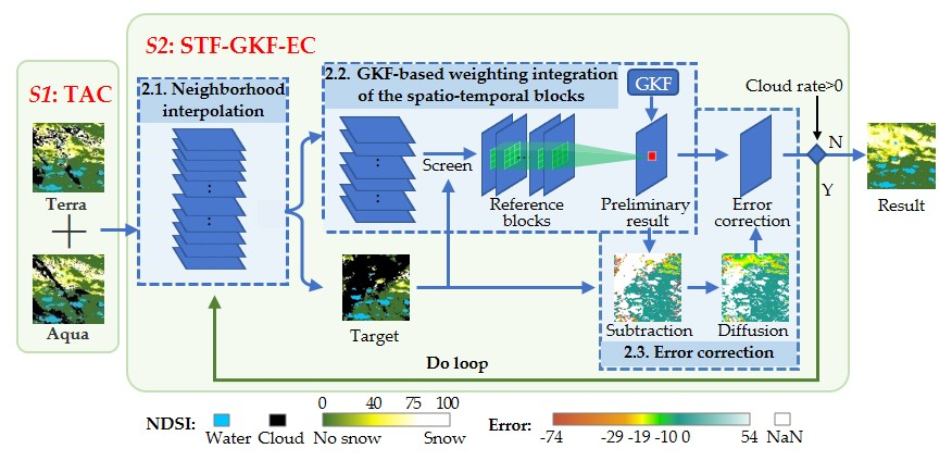
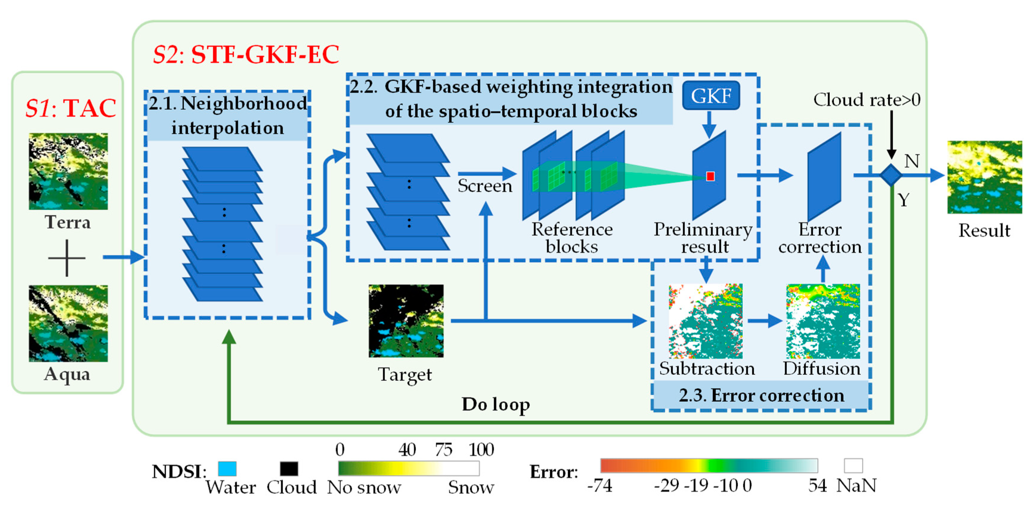
3.2. Spatio–Temporal Fusion Based on Gaussian Kernel Function and Error Correction (STF-GKF-EC)

Based on the output of the TAC, the remaining clouds are further removed by the second stage, i.e., STF-GKF-EC, which makes full use of the spatio–temporal information of the snow cover product. STF-GKF-EC includes three parts: (1) neighborhood interpolation; (2) GKF-based weighting integration of the spatio–temporal blocks; and (3) error correction. In order to ensure the accuracy, the three parts are performed recursively, to remove the clouds iteratively (see Figure 2). Taking a single cycle as an example, the details are provided in the following.

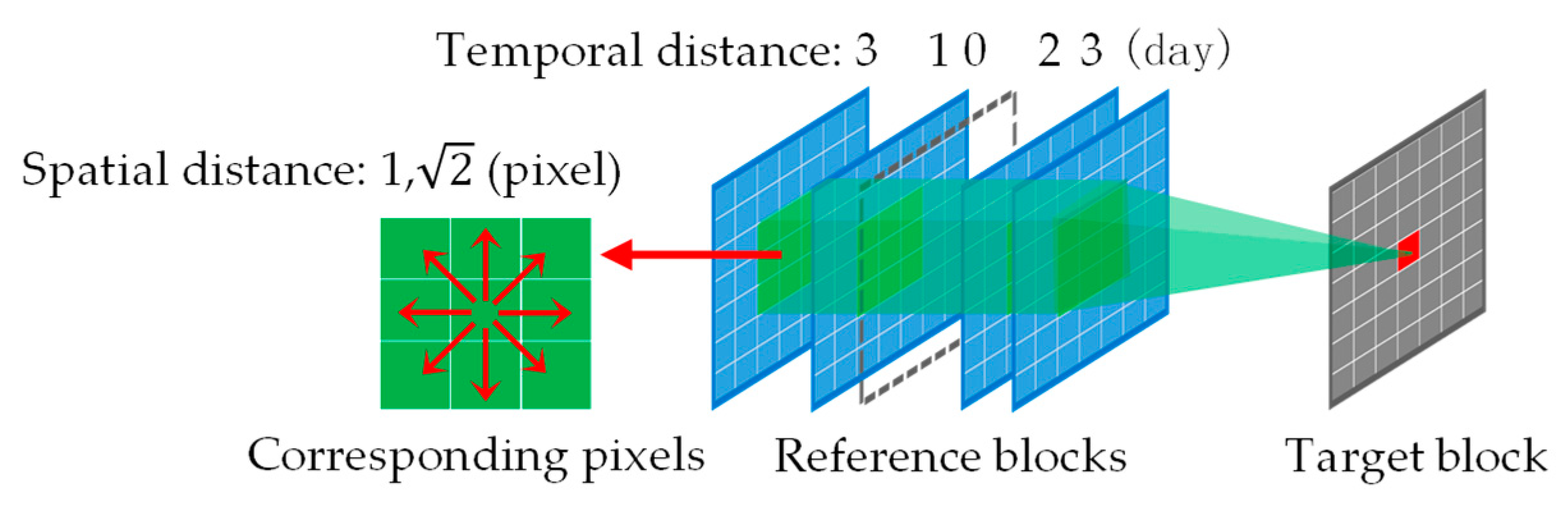
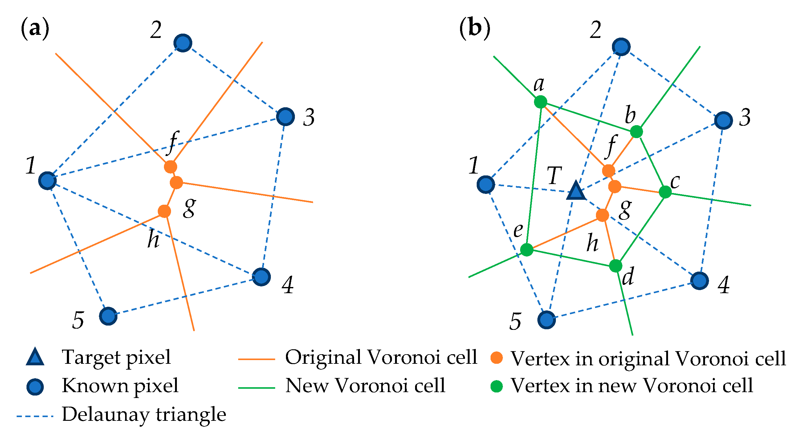
3.2.1. Neighborhood Interpolation

Neighborhood interpolation is a traditional method which has a high precision for filling small areas [22]. In order to ensure the reconstruction accuracy under cloud cover, only the cloud pixels adjacent to the known pixels are filled by the neighborhood interpolation in each cycle of STF-GKF-EC. As can be seen in Figure 3, for the $m$-th loop, the cloud pixels within a buffer no greater than $2m-1$ from known pixels, are interpolated by known pixels. Then, after the GKF-based weighting integration and error correction, if the cloud cover rate is larger than zero, the next loop begins to further remove the clouds (see Figure 2).

A variety of interpolation methods can be used in this step, the choice of which has little impact on the accuracy of the small-area cloud removal. In this paper, inverse distance weighting (IDW) with geographical features is applied, in which each cloud pixel is assigned a weighted average of the reliable clear-sky neighbors. Statistical analysis shows that when the elevation difference over the TP is greater than 50 m, there may be a large difference in snow conditions. Therefore, a pixel whose elevation difference from the target pixel is more than 50 m is considered unreliable and is excluded from the analysis. The formula can be expressed as follows:

$${\mathit{NDSI}}_i^T={\displaystyle \sum }_{n=1}^N{w}_{(i,n)}{\times \mathit{NDSI}}_{(i,n)}^T\cdots {\mathrm{where}w}_{\left(i,n\right)}=\frac{1/\Delta d_{(i,n)}}{{{\displaystyle \sum }}_{n=1}^N(1/\Delta d_{(i,n)})},$$

(1)

where ${\mathit{NDSI}}_i^T$ and ${\mathit{NDSI}}_{(i,n)}^T$ represent the NDSI of the $i$-th cloud pixel and its $n$-th neighboring reference pixel in the target image, respectively. $N$ is the total number of selected neighbors. $\Delta d_{(i,n)}$ is the spatial distance between the $n$-th reference pixel and the $i$-th target pixel, which is no more than a given threshold $2\times m$. In this way, the clouds near the clear-sky pixels can be removed efficiently and accurately, which is the basis for the next step.

3.2.2. GKF-based Weighting Integration of the Spatio–Temporal Blocks

To ensure accuracy, neighborhood interpolation is applied to recover a small range of cloud-covered pixels surrounding the non-cloud pixels. More importantly, GKF-based weighting integration of the spatio–temporal blocks is proposed to completely remove the residual clouds, which synthetically takes advantage of the spatio–temporal information in the reference images (see Figure 2). In short, it consists of block division, reference block selection, and weighted average calculation. The detailed description is as follows:

(1) Block division. Due to the complex terrain of the TP, the snow cover variation often presents regional inconsistency. In this regard, the minimum bounding rectangle of the TP is divided into b1 × b2 blocks uniformly, so that the subsequent steps can be performed block by block.

(2) Reference block selection. In order to ensure the reconstruction accuracy, only similar blocks are used as reference blocks. Since the variation of snow cover is rapid and complex, it is insufficient to measure the similarity by the temporal distance alone. Instead, the optimal reference blocks are selected from the candidate blocks within a given time window (Tw) via the combination of the correlation coefficient ($r$), non-cloud fraction ($f_n$), and temporal distance ($\Delta t$) as follows:

$$\{\begin{array}{cc}\mathrm{rule}1:r>0.7,\hfill & \hfill \mathrm{if}{f}_n^{C\&T}>0.3\\ \mathrm{rule}2:\max (\Delta t^{-1}+f_n^C),\hfill & \hfill \mathrm{others}\end{array},$$

(2)

where $f_n^{C\&T}$ represents the overlapping non-cloud fraction of the candidate block and the target block. $f_n^C$ is the non-cloud fraction of the candidate block. According to rule 1, a candidate block with a correlation coefficient to the target block higher than 0.7 is selected as a reference block, provided that $f_n^{C\&T}$ is high enough (0.3) to ensure that the calculated correlation coefficient is representative. The two thresholds were obtained from our experimental experience. In addition, if rule 1 fails, two reference blocks are selected by rule 2 to improve the efficiency of the cloud removal, with the sum of $\Delta t^{-1}$ and $f_n^C$ reaching a maximum in the 8 days preceding or following.

(3) Weighted average calculation. Firstly, based on the GKF, the weights of the corresponding cloud-free pixels in the reference blocks are calculated. As shown in Figure 4, each cloud pixel in the target block is preliminarily assigned the weighted average of the reference pixels, as shown in Equation (3):

$${\mathit{NDSI}}_j^P={\displaystyle \sum }_{t=1}^M{\displaystyle \sum }_{s=1}^N{w}_{(j,\mathrm{st})}{\times \mathit{NDSI}}_{(j,\mathrm{st})}^R{\mathrm{where}w}_{(j,\mathrm{st})}=\frac{w_{(j,t)}{\times w}_{(j,s)}}{{{\displaystyle \sum }}_{t=1}^M{{\displaystyle \sum }}_{s=1}^N\left(w_{(j,t)}{\times w}_{(j,s)}\right)},$$

(3)

where ${\mathit{NDSI}}_j^P$ is the preliminary NDSI of pixel $j$ in the target block. ${\mathit{NDSI}}_{(j,\mathrm{st})}^R$ represents the NDSI in the reference block. $M$ denotes the number of reference blocks, with each containing $N$ reference pixels. The weight $w_{(j,st)}$ of the reference pixel, which is determined by its temporal and spatial distance to the target pixel $j$, consists of the temporal weight $w_{(j,t)}$ and spatial weight $w_{(j,s)}$, as shown in Equation (4):

$$\{\begin{array}{c}{w}_{(j,t)}{=r}_t^2\times \exp \left(\frac{-(\Delta t_{(j,t)}^2)}{{2\sigma }_t^2}\right)\\ w_{(j,s)}=\exp \left(\frac{-(\Delta d_{(j,s)}^2)}{{2\sigma }_s^2}\right)\end{array},$$

(4)

where $r_t$ is the correlation coefficient between the reference block and the target block. In particular, it will be ignored when the reference block is selected by rule 2 (namely, $r_t=1$). $\Delta t_{(j,t)}$ and $\Delta d_{(j,s)}$ represent the normalized temporal distance and normalized spatial distance between the reference pixel and the target pixel, respectively. In addition, ${\sigma }_t$ and ${\sigma }_s$ are the corresponding standard deviations, which control the full width at half-maximum of each Gaussian curve.

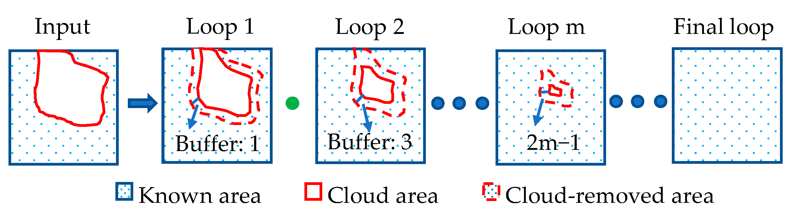
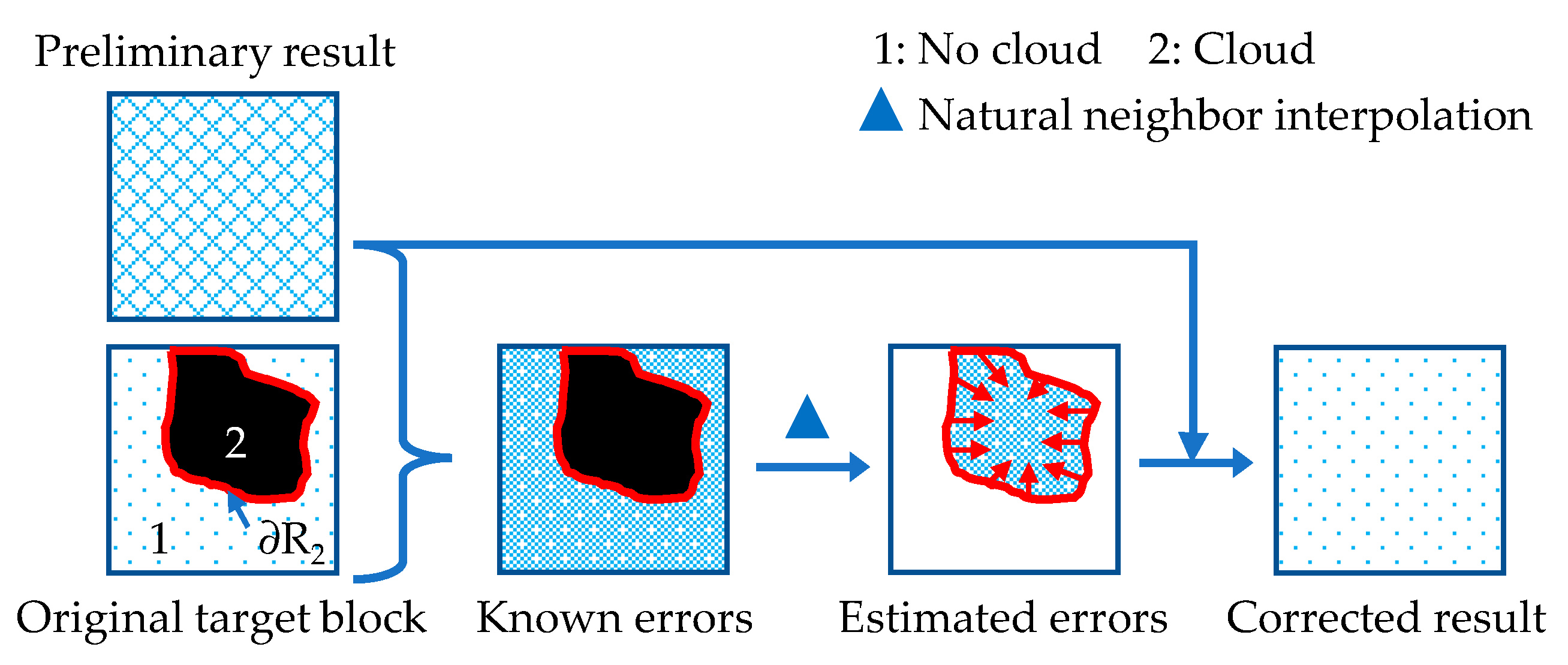
3.2.3. Error Correction

Based on the previous step, the preliminary cloud-removed result of each block can be obtained. However, large errors may occur during periods of rapid snow cover changes. It has been demonstrated that error correction with spatial correlation can further improve the effect of cloud removal [45]. Error correction is also adopted in this work (see Figure 2). According to Figure 5, the detailed process is described below.

(1) Known error calculation. As shown in Figure 5, the errors of the original cloud-free areas (i.e., region 1) are calculated by Equation (5):

$$E_1{=\mathit{NDSI}}_1^P{-\mathit{NDSI}}_1^T,$$

(5)

where ${\mathit{NDSI}}_1^P$ and ${\mathit{NDSI}}_1^T$ represent the NDSI in region 1 of the preliminary result and the original target block, respectively.

(2) Unknown error estimation. In consideration of the superiority in smooth approximation, the triangulation-based natural neighbor interpolation method [46] is adopted to estimate the errors in region 2. In particular, only the known errors on the boundary of region 2 (∂R₂) are utilized as a reference. The equation can be expressed as:

$$u^{\prime }(x,y)=\sum _{n=1}^N{\varphi }_{n}u(x_n,y_n),$$

(6)

where $u^{\prime }(x,y)$ is the estimation at $(x,y)$ based on the weighted combination of $N$ references ${u(x}_n{,y}_n)$. ${\varphi }_n$ is the weight associated with the known neighboring pixel $n$. Figure 6 shows the Voronoi diagrams for weight calculation. Specifically, Figure 6a shows the Voronoi diagram of pixels 1–5 based on the Delaunay triangles, in which f–h are the three vertices. When a target pixel T is included, its natural neighbors are those to which it is connected through the sides of the Delaunay triangles (pixels 1–5). A new Voronoi diagram is generated, as shown by the green line in Figure 6b, in which a–e are the five vertices in the Voronoi cell of pixel T. Taking pixel 1 as an example, the weight is given as follows:

$${\varphi }_1=\frac{A_{\mathit{afghe}}}{A_{\mathit{abcde}}},$$

(7)

where $A_{\mathit{afghe}}$ is the overlapping area of the Voronoi cell of pixel 1 in Figure 6a and that of pixel T in Figure 6b. $A_{\mathit{abcde}}$ is the total area of the Voronoi cell of pixel T.

(3) Error correction. The corrected result is determined by the subtraction of the new errors from the preliminary result. After all the blocks are processed, the next loop of STF-GKF-EC begins until there is no cloud (see Figure 2).

3.3. Validation Method

The proposed method was evaluated in terms of classification accuracy and numerical precision. The details are provided below.

3.3.1. Classification Accuracy

The metrics used in the research to evaluate the classification accuracy are the overall accuracy (OA), the commission error (CE), the omission error (OE) [24], and the F-score (FS) [38].

Table 1. Description of the confusion matrix and definition of the validation metrics.

Truth\Result	Snow	No Snow
Snow	SS	SN
No snow	NS	NN
$\mathrm{OA}=\frac{SS+NN}{SS+SN+NS+NN}$	$\mathrm{CE}=\frac{NS}{SS+SN+NS+NN}$
$\mathrm{OE}=\frac{SN}{SS+SN+NS+NN}$	$\mathrm{FS}=\frac{2\times SS}{2\times SS+SN+NS}$

shows the confusion matrix on which all the metrics are based, as well as the definition of the metrics. Specifically, pixels with an NDSI greater than 0 are classified as snow [36]. In contrast, the others are considered as snow-free land surface.

3.3.2. Numerical Precision

The numerical precision is based on the mean absolute error (MAE) and root-mean-square error (RMSE), as shown in Equations (8) and (9). Furthermore, since the two indicators are greatly affected by the large proportion of snow-free surface, which makes them unrealistically low, MAE and RMSE for the snow-covered areas (MAE_S and RMSE_S) are utilized for a more comprehensive evaluation.

$$\mathrm{MAE}=\frac{{{\displaystyle \sum }}_{k=1}^K\left|x_{1,k}{-x}_{2,k}\right|}{K},$$

(8)

$$\mathrm{RMSE}=\sqrt{\frac{{{\displaystyle \sum }}_{k=1}^K{{(x}_{1,k}{-x}_{2,k})}^2}{K}},$$

(9)

where $x_{1,k}$ and $x_{2,k}$ denote the NDSI of pixel $k$ in the validation data and the cloud-removed results. $K$ is the number of all pixels in the evaluation area.

4. Results

This section describes the accuracy evaluation in the simulated experiment, in which the parameters were set as shown in

Table 2. The parameters in the Gaussian kernel function (GKF)-based weighting integration of the spatio–temporal blocks.

Parameter	Description	Value
b1 × b2	Block size.	7 × 12
Temporal window (Tw)	Candidate days before and after the target image.	±8 days
Neighboring window (Nw)	The number of reference pixels in the neighborhood.	8
Elevation constraint (EC)	Maximum elevation difference for the reference block.	50 m
Correlation constraint (CC)	Minimum correlation coefficient for the reference block.	0.7
[${\sigma }_s$, ${\sigma }_t$] (see Section 4.2.1)	The spatial and temporal parameters in the GKF.	[0.5, 0.5]

. Since the TAC has been widely demonstrated to have a high accuracy, only the accuracy of STF-GKF-EC was evaluated.

4.1. Accuracy Evaluation of STF-GKF-EC

The evaluation was based on the approach developed by Gafurov and Bárdossy [18]. Firstly, 10 images (see

Table 3. The quantitative evaluation results of the spatio–temporal fusion based on Gaussian kernel function and error correction (STF-GKF-EC) on the entire Tibetan Plateau (TP).

Dates	SF	CF	Classification Accuracy				Numerical Precision↓
			OA (%)↑	CE (%)↓	OE (%)↓	FS↑	MAE	RMSE	MAE_S	RMSE_S
24 March 2016	0.30	0.67	92.05	2.39	5.57	0.88	5.15	11.88	9.96	14.01
17 April 2016	0.22	0.57	89.37	4.75	5.88	0.81	5.39	12.15	12.40	16.60
10 September 2016	0.05	0.75	90.37	4.96	4.67	0.50	3.03	9.55	15.44	20.14
01 October 2016	0.10	0.72	91.88	4.39	3.73	0.72	3.11	9.08	12.36	16.46
21 January 2017	0.16	0.67	92.89	3.23	3.88	0.82	3.11	8.32	10.24	13.98
31 March 2017	0.27	0.45	91.09	4.27	4.63	0.86	4.75	10.47	10.14	13.86
17 April 2017	0.19	0.50	94.29	3.61	2.10	0.87	3.09	8.08	9.96	13.46
08 May 2017	0.22	0.59	90.45	5.36	4.19	0.82	4.98	11.47	12.58	17.10
10 September 2017	0.07	0.88	91.52	5.70	2.78	0.62	2.90	8.96	14.81	19.13
27 September 2017	0.09	0.47	90.92	3.53	5.55	0.65	3.28	9.81	12.68	17.23
Average	0.17	0.63	91.48	4.22	4.30	0.75	3.88	9.98	12.06	16.20

Note: SF and CF represent the snow fraction of the evaluation area and the cloud fraction of the entire image, respectively. ↑ indicates that the higher the value, the better the precision; ↓ indicates the opposite. Bold red values and bold black values represent the best and worst values for each column, respectively. The NDSI ranges from 0, 10–100.

) with negligible cloud cover after the TAC from 2016/2017 were considered as “ground truth”. Cloud masks extracted from the images with high cloud coverage of 40–85% were applied to the “ground truth”. Then, the artificially cloud-covered images (called “observed data”) were reconstructed by STF-GKF-EC. Finally, the cloud-removed results were compared with the corresponding “ground truth”.

Since STF-GKF-EC was recursively performed, the clouds were removed iteratively. In the simulated experiment, the average cloud cover of the original data, the three intermediate products, and the final results on the 10 days were 62.61%, 26.58%, 2.38%, 0.09%, and 0, respectively. It should be noted that the number of iterations depends on the spatio–temporal cloud cover. The method automatically adjusts the number of iterations based on the remaining cloud coverage. For brevity, only two instances are shown in Figure 7. As can be seen from group (a), although the cloud cover of the “observed data” on 24 March 2016, is as high as 67%, STF-GKF-EC completely removes the clouds, and the cloud-free result shown in Figure 7 (a3) has a good consistency with the “ground truth”. Group (b) shows the results for 10 September 2017, with an extremely high cloud cover of 88% in the “observed data”. In this case, STF-GKF-EC restores the high values in snow-covered areas and retains the normal low values in snow-free areas. However, there are also a few misclassified pixels in the cloud removal result, mainly in the southeast of Brahmaputra and the interior of Qaidam. In these areas, the original reference images misidentified salt lakes, clouds, etc. as snow, leading to commission of the results. On the whole, the proposed method can remove all the clouds and restore the snow patterns with a high reliability.

To further verify the experimental results, the details of the red rectangular areas A3 and A4 (see Figure 7) are displayed in Figure 8. For group (a), it is clear that the result in (a3) is very pleasing, restoring the detailed information of the snow cover and preserving the spatial continuity with the original NDSI. As for group (b), the snow patterns of the cloud-removed result in (b3) are similar to those of the “ground truth” in (b1). However, some misclassified pixels can be observed at the edge of the snow cover (see the black rectangular areas). The reason is that the reference information is scarce owing to the continuous cloud presence in both the time sequence and the spatial neighborhood. In general, when there is no effective information in the adjacent five days during the period of snow accumulation or ablation, the reconstruction accuracy will be relatively poor in the area without the neighborhood information. Overall, STF-GKF-EC can recover all the NDSI of cloud-contaminated pixels, with a high agreement with the “ground truth”.

In addition, the quantitative evaluation results for the 10 simulated images are shown in Table 3. On the one hand, in terms of the classification accuracy, STF-GKF-EC obtains the robust OA ranging from 89.37% to 94.29%. The average OA reaches 91.48%, of which 4.22% is overestimated and 4.30% is underestimated. The FS varies from 0.50 to 0.88, which is basically consistent with the increase of the snow fraction. On the other hand, for the numerical precision, the average MAE and RMSE of the cloud-removed results are 3.88 and 9.98, compared with the “ground truth”. Moreover, the average MAE_S and RMSE_S reach 12.06 and 16.20, respectively. That is to say, STF-GKF-EC can also achieve a satisfactory numerical precision in snow-covered areas. From this comprehensive comparison, almost all the indicators suggest that 17 April 2017, has the highest accuracy. However, different conclusions about the most inaccurate day are obtained according to the different indicators. Since the snow fraction on 10 September 2016, is extremely low, the FS, MAE_S, and RMSE_S magnify the errors to some extent, as they only consider snow-covered areas. Hence, based on the OA, MAE, and RMSE of all areas, we conclude that the accuracy of the cloud removal for 17 April 2016, is relatively poor. The reason is that continuous cloud cover in time and space occurs during the snowmelt period. In summary, STF-GKF-EC can achieve satisfactory classification accuracy and numerical precision in both snow-covered and snow-free areas during all year.

In general, iterative processing can lead to error propagation. Therefore, the relation between the number of iterations and the accuracy of cloud removal was investigated.

Table 4. The relation between the number of iterations and the accuracy of cloud removal.

Number of Iterations	SF	CF	Classification Accuracy				Numerical Precision↓
			OA (%)↑	CE (%)↓	OE (%)↓	FS↑	MAE	RMSE	MAE_S	RMSE_S
1	0.14	0.23	93.66	3.52	2.82	0.78	2.69	7.74	10.31	14.09
2	0.17	0.02	92.01	4.22	3.77	0.78	3.64	9.40	11.67	15.70
3	0.17	3.62 × 10−7	91.86	4.29	3.86	0.77	3.69	9.52	11.73	15.79
4	0.17	0	91.86	4.29	3.86	0.77	3.69	9.52	11.73	15.79

shows the average accuracy of each iteration of 6 simulated images in 2017. The OA drops from 93.66% after the first iteration to 91.86% after the fourth iteration. For the numerical precision, the MAE and RMSE increase by 1.00 and 1.78, respectively. The MAE_S and RMSE_S increase to 11.73 and 15.79, respectively. It reveals that as the number of iterations increases, the classification accuracy and numerical precision decrease. However, as stated above, the STF-GKF-EC synthetically utilizes the spatial and temporal information, so that the cloud removal efficiency is high and the number of iterations is small. In our experiments, even in summer with extremely high cloud coverage, the number of iterations is no more than seven. Therefore, the final error of the STF-GKF-EC is still small.

4.2. Discussion of STF-GKF-EC

As stated above, the STF-GKF-EC can achieve robust accuracy for cloud removal. The two advantages of this method are: (1) the spatial and temporal weights are unified by the GKF; and (2) the estimation errors are reduced by the error correction. For the two aspects, there are two issues to be discussed.

4.2.1. Parameter Determination

Since the spatial and temporal weights are unified by the GKF, the two parameters in the GKF need to be determined. Figure 9 shows the results of the parametric test for 24 March 2016, and 1 October 2016, including the RMSE, RMSE_S, and OA values corresponding to different matrices of [${\sigma }_s$, ${\sigma }_t$]. For simplicity, the parameter testing was only performed on “A1” and “A2” (see Figure 1), and error correction in STF-GKF-EC was omitted. The different colors and vertices of the polygon represent different spatial and temporal parameters, respectively. The vertical comparison shows that the impact of the spatial parameter on the accuracy is highly consistent in the different regions, while that of the temporal parameter is relatively complex. From the horizontal perspective, as the value of the spatial parameter increases, the OA and RMSE are improved, while the RMSE_S is worse. The reason is that the OA and RMSE are significantly affected by the proportion of snow-free areas, while RMSE_S is the opposite. Specifically, when the spatial parameter value is 0.5 or 0.7, the OA and RMSE of both regions show a higher accuracy, while a value of 0.5 performs significantly better than 0.7 in terms of RMSE_S on A2. Therefore, ${\sigma }_s=0.5$ is regarded as the optimal parameter setting. In addition, when the temporal parameter value is set as 0.5, the RMSE and RMSE_S of “A1” and the RMSE_S of “A2” show good performance. Thus, the parameter matrix [0.5, 0.5] is recommended in STF-GKF-EC.

4.2.2. Effect of Error Correction

As stated above, the error correction further improves the numerical accuracy and spatial consistency of the NDSI data, especially during periods of rapid changes in snow cover. The effect of the error correction is affected by the quantity and distribution of the original effective data. Figure 10 shows three specific effects (groups (c)–(e)) extracted from the results for 24 March 2016, where the cloud removal results of STF-GKF-EC are compared with those of the method without error correction. Group (c) presents an example with an excellent correction effect. Since the snow cover in this area varies greatly over a few days, the NDSI values filled with the information of the reference images are significantly underestimated, as shown in (c3). In this case, based on the original effective information of the target image, the error correction can greatly improve the reconstruction accuracy. However, group (d) reveals that the correction is likely to be insufficient when the spatial information is scarce. In addition, original effective data with an extremely uneven spatial distribution may introduce incorrect error information, due to the lack of representativeness, resulting in excessive correction, as shown in group (e). The NDSI in (e3) is slightly overestimated at the edge of the snow-covered areas, and is covered by clouds in other snow-covered areas. Accordingly, nearby cloud-covered areas are mistakenly considered to be overestimated, thus correcting these overestimates and leading to underestimation. In general, although there are some insufficient and excessive corrections, the error correction can effectively eliminate the temporal errors introduced by the reference images, indicating that it is an essential component of the proposed method.

5. Snow Cover Variability

Based on the cloud-removed results of the proposed method, the variability of snow cover over the TP during 2001–2017 was analyzed from three aspects. Specifically, the intra-annual and inter-annual variabilities were revealed with respect to different elevation zones and/or subranges. The response of snow cover variability to temperature and precipitation in the different subranges was also investigated.

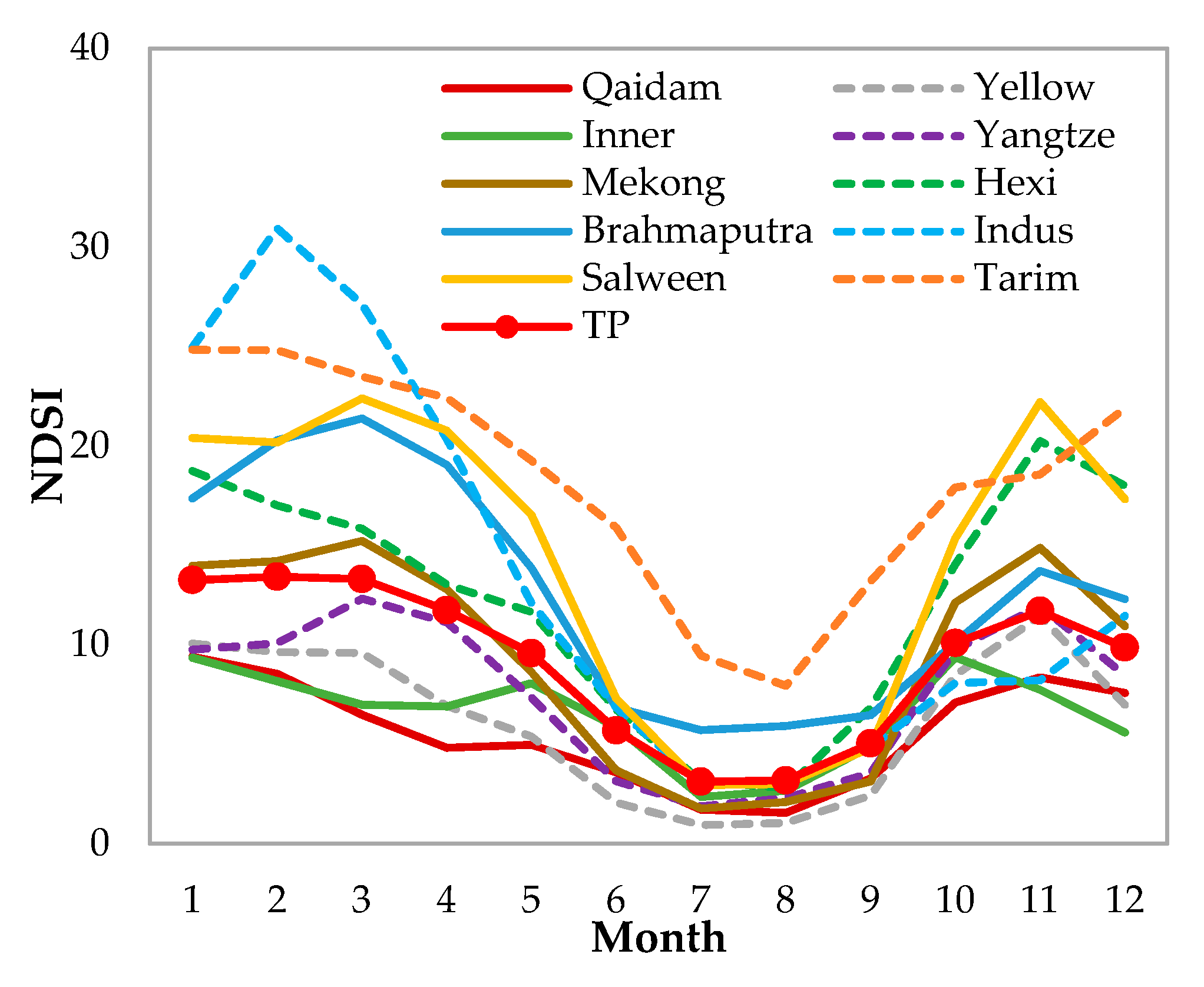
5.1. Intra-Annual Variability of Snow Cover

The intra-annual variability was analyzed at both the daily and monthly scales. First, the average daily snow fraction (the ratio of NDSI greater than 0) and the average daily NDSI for snow-covered areas in a hydrological year are shown in Figure 11 and Figure 12, respectively. The gray error bars represent the standard deviation. It can be seen that the daily snow fraction over the TP fluctuates greatly, with a maximum of 34.87% on 20 January and a minimum of 8.45% on 5 August. In comparison, the average daily NDSI for the snow-covered areas rises earlier and falls later, with a maximum of 46.11 on 24 October and a minimum of 31.80 on 9 August. In other words, on the one hand, snow accumulation first occurs in areas with high NDSI values, and then spreads to snow-free areas. On the other hand, snow ablation starts from areas with low NDSI values, and then moves to areas with high NDSI values. However, in general, their changes are highly consistent, with a correlation coefficient of 0.91.

Furthermore, the analysis at the monthly scale considers different elevations and subregions. Figure 13 shows the average monthly NDSI at different elevation zones. On the TP, this reveals that a large proportion of the snow cover lasts from October to May, with a peak of 13.43 in February. Rapid accumulation and ablation occur in September/October and May/June, respectively. Moreover, a slight decrease appears in December, which is mainly due to the dryness in winter over the TP. However, the snow cover variation is different in the different elevation zones. In areas with an altitude of less than 4000 m, the period of snow presence is fairly short, mainly in January and February. Meanwhile, the areas above 6000 m are almost permanently covered with snow, where the lowest average NDSI is as high as 50.05. This is a large difference compared with the areas in the lower elevation zone. Furthermore, since about half of the TP has an altitude of 4000–5000 m, the intra-annual snow variation curve of the areas is similar to that of the entire TP. However, its maximum appears in March, which is the same as the areas with an altitude of 5000–6000 m.

In view of the different subregions (see Figure 1), there are also some commonalities and individualities in the intra-annual snow cover variation, as shown in Figure 14. On the one hand, all the subregions quickly accumulate snow in September/October. Except for Tarim and Indus, all subregions have a lower NDSI in December. Furthermore, the snow cover in each subregion reaches a minimum in July/August. On the other hand, snowmelt onset occurs between January and March, depending on the subregion. Hexi, for example, has relatively high snow cover in November, but the snow begins to melt as early as January. The snow in Indus is almost exclusively concentrated between January and March, and then drops sharply to a very low proportion. In addition, it can be noticed that the Inner subregion has three peaks, which occur in January, May, and October, respectively. In contrast, Tarim, with a high average NDSI, has a smoother snow cover curve, retaining some permanent snow in summer. Moreover, the intra-annual snow variation curves of the Mekong and Yangtze river basins are the closest to that of the entire TP.

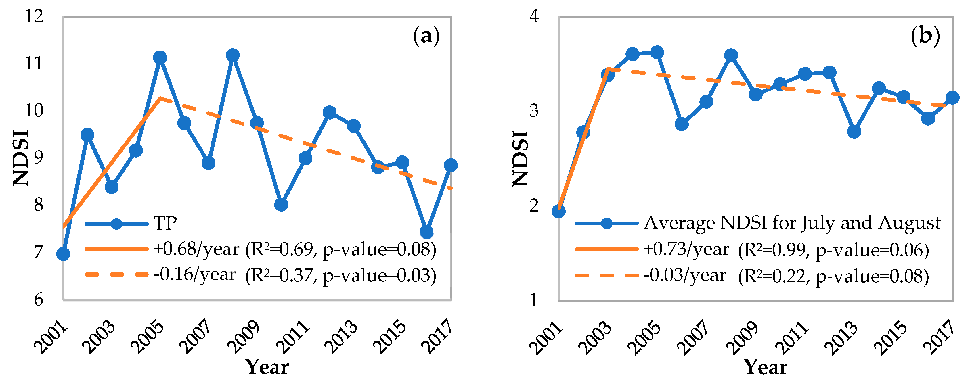
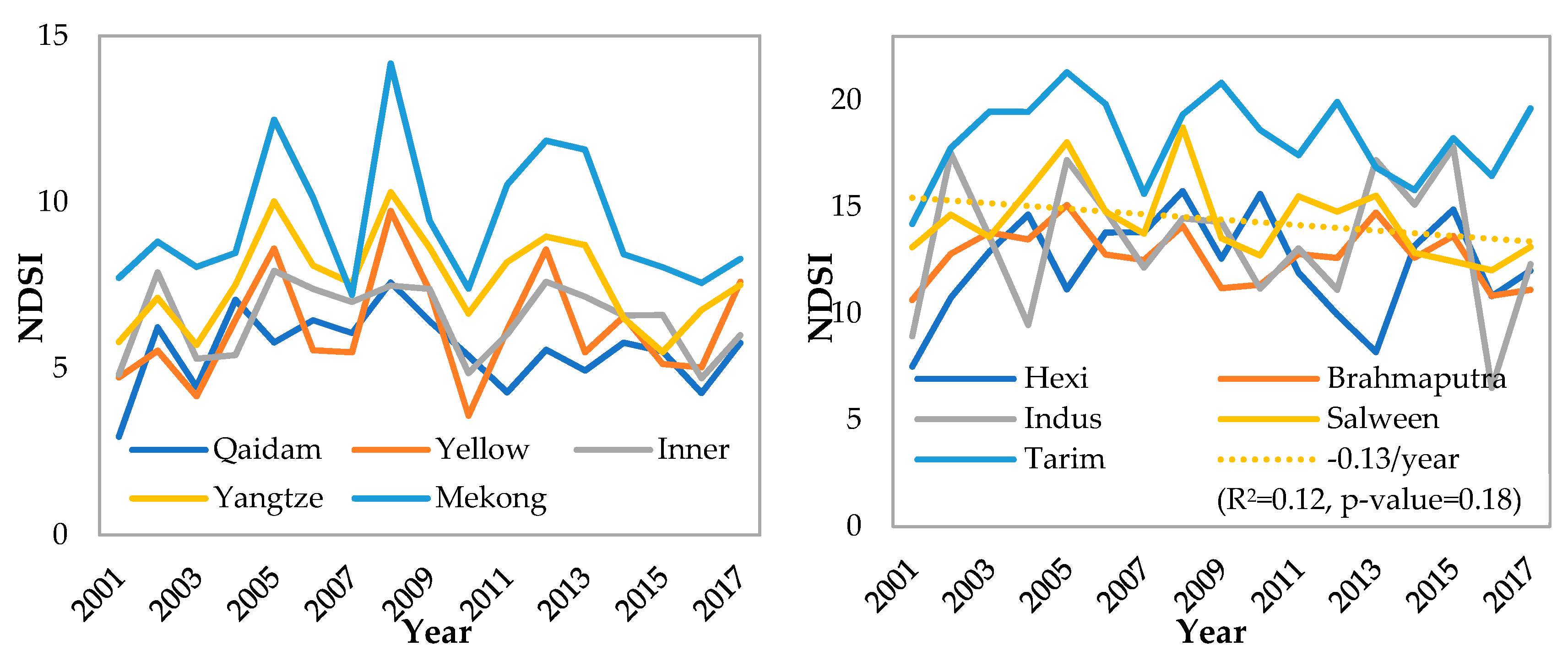
5.2. Inter-Annual Variability of Snow Cover

Based on the cloud-free NDSI product, the inter-annual snow cover variability was also analyzed. The variation trend over the entire TP is described by a piecewise linear regression model [35,47]:

$${\mathit{NDSI}}_t=\{\begin{array}{ll}{\beta }_0{+\beta }_{1}t+\epsilon ,& t\le t_0\\ {\beta }_0{+\beta }_1{t+\beta }_2{(t-t}_0)+\epsilon ,& t>t_0\end{array},$$

(10)

where ${\mathit{NDSI}}_t$ denotes the NDSI in the $t$-th year, $\epsilon$ is the residual error, $t_0$ is the breakpoint determined by the least-squares error, namely $t_0=\mathit{argmin}({\parallel \epsilon \parallel }^2)$, ${\beta }_i$ is the regression coefficient, and ${\beta }_1$ and ${\beta }_1{+\beta }_2$ are the slopes of the two equations, which can quantify the trends before and after the breakpoint.

Firstly, the annual averages of NDSI over the entire TP from 2001 to 2017 are shown in Figure 15a. An apparent increasing trend can be observed during 2001–2005, as well as a slight decreasing trend during 2005–2017. Using the piecewise linear regression model, the trends are determined as being +0.68/year and −0.16/year, respectively. The trends are statistically significant (α = 0.10). Over the past decade, the annual average NDSI has fallen from more than 11 to about eight. In addition, since the snow cover reaches its lowest value in July and August, we can assume that the snow cover during this period is permanent snow cover. Figure 15b shows the changes of average NDSI for July and August over the 17 years. It can be seen that, after a rapid rise during 2001–2003, a slight decreasing trend of 0.03/year has lasted for 14 years.

Moreover, according to the magnitude of the average NDSI, the 10 subregions over the TP are ranked as Qaidam, Yellow, Inner, Yangtze, Mekong, Hexi, Brahmaputra, Indus, Salween, and Tarim (see Figure 16). This reveals that the snow cover is high in the western, southern, and northern margins of the TP, and relatively low in the central and eastern regions. In addition, the snow cover in each subregion has fluctuated greatly over the 17 years. The linear regression equation of Salween has the smallest slope of −0.13/year. However, this trend is not statistically significant (α = 0.10).

To further investigate the correlation of the inter-annual snow cover variation between the subregions and the entire TP,

Table 5. The snow cover variability on the TP and the 10 subregions during 2001–2017.

Indicator	Qaidam	Yellow	Inner	Yangtze	Mekong	Hexi	Brahmaputra	Indus	Salween	Tarim	TP
Avg.	5.56	6.22	6.49	7.63	9.43	12.31	12.71	13.33	14.40	18.28	9.14
Std.	1.13	1.68	1.13	1.42	2.04	2.40	1.35	3.24	1.88	1.98	1.11
CV	0.20	0.27	0.17	0.19	0.22	0.20	0.11	0.24	0.13	0.11	0.12
Pixel (104)	102	97	264	182	36	25	139	37	45	75	1031
Elevation (m)	3575	3798	4981	4201	4328	3839	4590	5002	4568	4437	4354
R (TP)	0.72 (0.001)	0.78 (0.000)	0.86 (0.000)	0.85 (0.000)	0.84 (0.000)	0.21 (0.429)	0.69 (0.002)	0.62 (0.008)	0.82 (0.000)	0.65 (0.004)	-

Note: The indicators represent the average NDSI (Avg.), standard deviation (Std.), coefficient of variation (CV), number of pixels (Pixel), regional-average elevation (Elevation), correlation coefficient (R) and p-value.

lists some indicators describing the variation and regional topography. On the one hand, the inter-annual snow cover variation of the four subregions of Inner, Yangtze, Mekong, and Salween has a high consistency with that of the TP, obtaining a correlation coefficient of above 0.82. On the other hand, the specific variability of the snow cover shows significant regional inconsistency. For example, Tarim has the largest average NDSI of 18.28, which is twice that of the TP; however, their average elevation difference is only 83 m. In comparison, the snow cover variability over the Mekong subregion with a similar average elevation, is more consistent with the entire TP. At the same time, significantly inconsistent variability can be observed in Hexi. Furthermore, in terms of the standard deviation and coefficient of variation, the snow cover changes most dramatically in the Indus valley, followed by Hexi, Mekong, and the Yellow River basin. On the whole, the inter-annual variations of the different subregions are highly inconsistent.

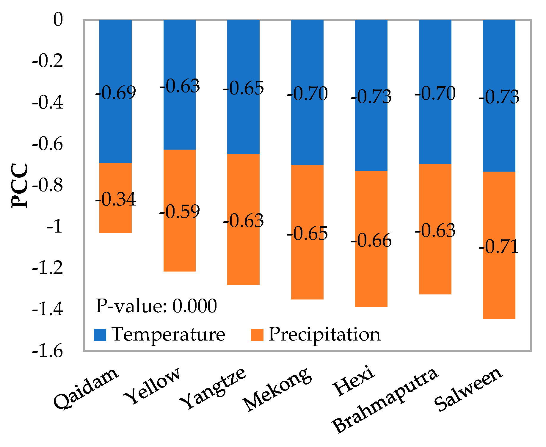
5.3. Response of Snow Cover to Climate Change

As we know, snow is very sensitive to climate change, of which the most important factors are temperature and precipitation. Accordingly, based on the meteorological station data, the effects of temperature and precipitation on the intra-annual and inter-annual variabilities of snow cover were analyzed. As the meteorological stations are mainly distributed in the east of the TP, this analysis only covered the seven subregions in this area. From the perspective of intra-annual variability, Figure 17 reveals that the snow cover over the TP has a significant negative correlation with temperature and precipitation. In all the subregions, the impact of temperature on the snow cover variation is greater than that of precipitation, and the degree is slightly magnified as the snow cover increases. In particular, the monthly NDSI in Qaidam has little correlation with precipitation. The reason is that the precipitation of Qaidam is extremely low, with an average of about 8.6 mm over the 17 years according to the four meteorological stations. Generally speaking, the intra-annual snow cover variation over the TP is mainly controlled by temperature rather than precipitation.

According to the Pearson correlation coefficients (PCCs) of the average monthly NDSI and temperature/precipitation from 2001 to 2016,

Table 6. The Pearson correlation coefficients of the inter-annual variation of the monthly NDSI and temperature/precipitation from 2001–2016.

Month	Temperature							Precipitation
	A	B	C	D	E	F	G	A	B	C	D	E	F	G
Jan	−0.26	−0.41	−0.49	−0.49	−0.36	−0.62	0.01	0.78	0.76	0.85	0.78	0.83	0.61	0.49
Feb	−0.47	−0.83	−0.75	−0.06	−0.56	−0.79	−0.23	0.39	0.51	0.29	0.36	0.38	0.58	−0.17
Mar	0.04	−0.37	−0.62	−0.16	−0.18	−0.37	−0.24	0.67	0.54	0.37	0.54	0.33	−0.49	−0.13
Oct	0.13	−0.30	−0.37	−0.33	−0.10	−0.52	−0.43	0.73	0.38	0.36	0.44	0.77	0.69	0.86
Nov	−0.21	−0.32	−0.62	−0.29	−0.33	−0.32	−0.63	0.44	0.60	0.18	0.23	0.18	0.31	−0.07
Dec	0.18	−0.14	−0.18	−0.25	−0.30	0.01	−0.45	0.44	0.55	0.16	0.30	0.52	0.43	0.40
Oct–Mar	−0.16 (0.56)	−0.62 (0.01)	−0.44 (0.09)	0.04 (0.89)	−0.11 (0.68)	−0.27 (0.31)	−0.29 (0.27)	0.72 (0.00)	0.42 (0.11)	0.26 (0.33)	0.39 (0.14)	0.46 (0.08)	0.56 (0.03)	0.49 (0.05)

Note: A–G represent Qaidam, Yellow, Yangtze, Mekong, Hexi, Brahmaputra, and Salween, respectively. The p-values are in parentheses.

describes the correlation between the inter-annual variation of snow cover and the climatic factors. It can be seen that temperature has little effect on the inter-annual snow cover variation, with only February showing a significant negative correlation. Precipitation, in contrast, is typically positively correlated with the snow cover variation, especially in January and October. Moreover, the overall PCCs from October to March also indicate that precipitation has a greater effect on the inter-annual variability than temperature. However, the regional inconsistency is also significant, for example, the correlation coefficient is relatively low around the Yangtze River. In the Salween River basin, there is even an alternating positive/negative correlation. As a result, compared to the intra-annual variability in snow cover, inter-annual variability in snow cover exhibits a weaker correlation with both temperature and precipitation.

6. Conclusions

The investigation of snow cover variability over the TP is of great importance. MODIS snow products are widely adopted to monitor the snow cover variation over the TP, owing to the appropriate temporal and spatial resolutions. However, removing cloud cover has been a challenge of snow monitoring due to the extremely complex topography over the TP. Therefore, this paper is intended as a precedent for producing cloud-free MODIS NDSI product using spatio–temporal information. The proposed two-stage spatio–temporal fusion framework includes an adjusted Terra and Aqua combination (TAC) and a spatio–temporal fusion based on Gaussian kernel function and error correction (STF-GKF-EC). Firstly, the TAC based on an adjusted priority scheme, is used as the first stage to reduce the cloud cover. STF-GKF-EC is then implemented according to the following procedure: (1) neighborhood interpolation; (2) GKF-based weighting integration of the spatio–temporal blocks; and (3) error correction. It should be noted that this process is recursively performed on the NDSI product until no cloud-covered pixels remain. Since the TAC has been extensively demonstrated to be highly accurate, only STF-GKF-EC was evaluated in this paper. The simulated experiment suggests that STF-GKF-EC can obtain an average OA of 91.48%. In addition, the MAE and the MAE for snow-covered areas (MAE_S) are 3.88 and 12.06, respectively. Overall, STF-GKF-EC has three advantages: (1) it takes into account regional inconsistency through the block processing; (2) it simultaneously considers the spatial and temporal information based on the unified spatio–temporal weight; and (3) it further improves the accuracy by the error correction. Nevertheless, there are still some disadvantages: (1) STF-GKF-EC may lead to a few misclassifications at the edge of the snow cover; and (2) it is difficult to recover the cloud-covered pixels with a high precision when continuous cloud cover appears in the snow accumulation or ablation period. For our future work, remote sensing data from different sensors, such as Sentinel data, will be fused to produce higher-quality NDSI products. The key is to improve the accuracy of the areas covered by continuous cloud during the snow accumulation and ablation.

Based on the cloud-removed product, the variability of snow cover over the TP was analyzed. It reveals that the snow cover over the TP is relatively high from October to May. The average NDSI during the snow period reaches a trough in December and a peak in February/March. The snow cover over the TP presents an upward trend of 0.68/year from 2001 to 2005, and a downward trend of 0.16/year from 2005 to 2017. Moreover, on the one hand, the explanatory power of temperature for the intra-annual snow cover variation is higher than that of precipitation. On the other hand, precipitation has a relatively significant positive effect on the inter-annual variation. With global warming, monitoring the variability of snow cover is an urgent concern. Undoubtedly, the decreasing trend of snow cover over the TP after 2005 is a warning signal. Therefore, more research is needed on this issue.

References

1. Kang, S.; Xu, Y.; You, Q.; Flügel, W.A.; Pepin, N.; Yao, T. Review of climate and cryospheric change in the Tibetan Plateau. Environ. Res. Lett. 2010, 5, 015101. [Google Scholar] [CrossRef]
2. Konzelmann, T.; Ohmura, A. Radiative fluxes and their impact on the energy balance of the Greenland ice sheet. J. Glaciol. 1995, 41, 490–502. [Google Scholar] [CrossRef] [Green Version]
3. Hall, D.K.; Riggs, G.A.; Salomonson, V.V. Development of methods for mapping global snow cover using moderate resolution imaging spectroradiometer data. Remote Sens. Environ. 1995, 54, 127–140. [Google Scholar] [CrossRef]
4. Şorman, A.Ü.; Akyürek, Z.; Şensoy, A.; Şorman, A.A.; Tekeli, A.E. Commentary on comparison of MODIS snow cover and albedo products with ground observations over the mountainous terrain of Turkey. Hydrol. Earth Syst. Sci. 2007, 11, 1353–1360. [Google Scholar] [CrossRef] [Green Version]
5. Barnett, T.P.; Adam, J.C.; Lettenmaier, D.P. Potential impacts of a warming climate on water availability in snow-dominated regions. Nature 2005, 438, 303–309. [Google Scholar] [CrossRef] [PubMed]
6. Baghdadi, N. Capability of Multitemporal ERS-1 SAR Data for Wet-Snow Mapping. Remote Sens. Environ. 1997, 60, 174–186. [Google Scholar] [CrossRef]
7. Che, T.; Dai, L.; Zheng, X.; Li, X.; Zhao, K. Estimation of snow depth from passive microwave brightness temperature data in forest regions of northeast China. Remote Sens. Environ. 2016, 183, 334–349. [Google Scholar] [CrossRef]
8. Liang, T.G.; Zhang, X.T.; Xie, H.J.; Wu, C.X.; Feng, Q.S.; Huang, X.D.; Chen, Q.G. Toward improved daily snow cover mapping with advanced combination of MODIS and AMSR-E measurements. Remote Sens. Environ. 2008, 112, 3750–3761. [Google Scholar] [CrossRef]
9. Romanov, P.; Gutman, G.; Csiszar, I. Automated Monitoring of Snow Cover over North America with Multispectral Satellite Data. J. Appl. Meteorol. 2000, 39, 1866–1880. [Google Scholar] [CrossRef]
10. Dietz, A.J.; Kuenzer, C.; Gessner, U.; Dech, S. Remote sensing of snow—A review of available methods. Int. J. Remote Sens. 2012, 33, 4094–4134. [Google Scholar] [CrossRef]
11. Crawford, C.J.; Manson, S.M.; Bauer, M.E.; Hall, D.K. Multitemporal snow cover mapping in mountainous terrain for Landsat climate data record development. Remote Sens. Environ. 2013, 135, 224–233. [Google Scholar] [CrossRef] [Green Version]
12. Hüsler, F.; Jonas, T.; Riffler, M.; Musial, J.P.; Wunderle, S. A satellite-based snow cover climatology (1985–2011) for the European Alps derived from AVHRR data. Cryosphere 2014, 8, 73–90. [Google Scholar] [CrossRef]
13. Simic, A.; Fernandes, R.; Brown, R.; Romanov, P.; Park, W. Validation of VEGETATION, MODIS, and GOES+ SSM/I snow-cover products over Canada based on surface snow depth observations. Hydrol. Process. 2004, 18, 1089–1104. [Google Scholar] [CrossRef]
14. Li, X.H.; Jing, Y.H.; Shen, H.F.; Zhang, L.P. The recent developments in cloud removal approaches of MODIS snow cover product. Hydrol. Earth Syst. Sci. 2019, 23, 2401–2416. [Google Scholar] [CrossRef] [Green Version]
15. Ciancia, E.; Coviello, I.; Di Polito, C.; Lacava, T.; Pergola, N.; Satriano, V.; Tramutoli, V. Investigating the chlorophyll-a variability in the Gulf of Taranto (North-western Ionian Sea) by a multi-temporal analysis of MODIS-Aqua Level 3/Level 2 data. Cont. Shelf Res. 2018, 155, 34–44. [Google Scholar] [CrossRef]
16. Li, X.; Shen, H.; Zhang, L.; Zhang, H.; Yuan, Q.; Yang, G. Recovering Quantitative Remote Sensing Products Contaminated by Thick Clouds and Shadows Using Multitemporal Dictionary Learning. IEEE Trans. Geosci. Remote Sens. 2014, 52, 7086–7098. [Google Scholar]
17. Parajka, J.; Bloschl, G. Spatio-temporal combination of MODIS images—Potential for snow cover mapping. Water Resour. Res. 2008, 44, 1–13. [Google Scholar] [CrossRef]
18. Gafurov, A.; Bárdossy, A. Cloud removal methodology from MODIS snow cover product. Hydrol. Earth Syst. Sci. 2009, 13, 1361–1373. [Google Scholar] [CrossRef] [Green Version]
19. Wang, X.; Zheng, H.; Chen, Y.; Liu, H.; Liu, L.; Huang, H.; Liu, K. Mapping snow cover variations using a MODIS daily cloud-free snow cover product in northeast China. J. Appl. Remote Sens. 2014, 8, 084681. [Google Scholar] [CrossRef]
20. Paudel, K.P.; Andersen, P. Monitoring snow cover variability in an agropastoral area in the Trans Himalayan region of Nepal using MODIS data with improved cloud removal methodology. Remote Sens. Environ. 2011, 115, 1234–1246. [Google Scholar] [CrossRef]
21. Parajka, J.; Pepe, M.P.L.; Rampini, A.; Rossi, S.; Bloschl, G. A regional snow-line method for estimating snow cover from MODIS during cloud cover. J. Hydrol. 2010, 381, 203–212. [Google Scholar] [CrossRef]
22. Tong, J.; Déry, S.J.; Jackson, P.L. Topographic control of snow distribution in an alpine watershed of western Canada inferred from spatially-filtered MODIS snow products. Hydrol. Earth Syst. Sci. 2009, 13, 319–326. [Google Scholar] [CrossRef] [Green Version]
23. López-Burgos, V.; Gupta, H.V.; Clark, M. Reducing cloud obscuration of MODIS snow cover area products by combining spatio-temporal techniques with a probability of snow approach. Hydrol. Earth Syst. Sci. 2013, 17, 1809–1823. [Google Scholar] [CrossRef] [Green Version]
24. Akyürek, Z.; Hall, D.K.; Riggs, G.A.; Sensoy, A. Evaluating the utility of the ANSA blended snow cover product in the mountains of eastern Turkey. Int. J. Remote Sens. 2010, 31, 3727–3744. [Google Scholar] [CrossRef]
25. Brown, R.; Derksen, C.; Wang, L. A multi-data set analysis of variability and change in Arctic spring snow cover extent, 1967–2008. J. Geophys. Res. Space Phys. 2010, 115, 1–16. [Google Scholar] [CrossRef]
26. Chen, X.; Long, D.; Liang, S.; He, L.; Zeng, C.; Hao, X.; Hong, Y. Developing a composite daily snow cover extent record over the Tibetan Plateau from 1981 to 2016 using multisource data. Remote Sens. Environ. 2018, 215, 284–299. [Google Scholar] [CrossRef]
27. Gafurov, A.; Vorogushyn, S.; Farinotti, D.; Duethmann, D.; Merkushkin, A.; Merz, B. Snow-cover reconstruction methodology for mountainous regions based on historic in situ observations and recent remote sensing data. Cryosphere 2015, 9, 451–463. [Google Scholar] [CrossRef] [Green Version]
28. Gao, Y.; Xie, H.; Yao, T. Developing Snow Cover Parameters Maps from MODIS, AMSR-E, and Blended Snow Products. Photogramm. Eng. Remote Sens. 2011, 77, 351–361. [Google Scholar] [CrossRef]
29. He, G.; Feng, X.; Xiao, P.; Xia, Z.; Wang, Z.; Chen, H.; Li, H.; Guo, J. Dry and Wet Snow Cover Mapping in Mountain Areas Using SAR and Optical Remote Sensing Data. IEEE J. Sel. Top. Appl. Earth Obs. Remote Sens. 2017, 10, 2575–2588. [Google Scholar] [CrossRef]
30. Huang, X.; Deng, J.; Ma, X.; Wang, Y.; Feng, Q.; Hao, X.; Liang, T. Spatiotemporal dynamics of snow cover based on multi-source remote sensing data in China. Cryosphere 2016, 10, 2453–2463. [Google Scholar] [CrossRef] [Green Version]
31. Shen, H.; Li, X.; Cheng, Q.; Zeng, C.; Yang, G.; Li, H.; Zhang, L. Missing Information Reconstruction of Remote Sensing Data: A Technical Review. IEEE Geosci. Remote Sens. Mag. 2015, 3, 61–85. [Google Scholar] [CrossRef]
32. Shen, H.F.; Meng, X.C.; Zhang, L.P. An integrated framework for the spatio-temporal-spectral fusion of remote sensing images. IEEE Trans. Geosci. Remote Sens. 2016, 54, 7135–7148. [Google Scholar] [CrossRef]
33. Gascoin, S.; Hagolle, O.; Huc, M.; Jarlan, L.; Dejoux, J.F.; Szczypta, C.; Marti, R.; Sanchez, R. A snow cover climatology for the Pyrenees from MODIS snow products. Hydrol. Earth Syst. Sci. 2015, 19, 2337–2351. [Google Scholar] [CrossRef] [Green Version]
34. Dariane, A.B.; Khoramian, A.; Santi, E. Investigating spatiotemporal snow cover variability via cloud-free MODIS snow cover product in Central Alborz Region. Remote Sens. Environ. 2017, 202, 152–165. [Google Scholar] [CrossRef]
35. Li, X.H.; Fu, W.X.; Shen, H.F.; Huang, C.L.; Zhang, L.P. Monitoring snow cover variability (2000–2014) in the Hengduan Mountains based on cloud-removed MODIS products with an adaptive spatio-temporal weighted method. J. Hydrol. 2017, 551, 314–327. [Google Scholar] [CrossRef]
36. Riggs, G.A.; Hall, D.K. MODIS Snow Products Collection 6 User Guide. Available online: https://nsidc.org/sites/nsidc.org/files/ files/MODIS-snow-user-guide-C6.pdf (accessed on 9 July 2019).
37. Crawford, C.J. MODIS Terra collection 6 fractional snow cover validation in mountainous terrain during spring snowmelt using Landsat TM and ETM. Hydrol. Process. 2015, 29, 128–138. [Google Scholar] [CrossRef]
38. Zhang, H.; Zhang, F.; Zhang, G.; Che, T.; Yan, W.; Ye, M.; Ma, N. Ground-based evaluation of MODIS snow cover product V6 across China: Implications for the selection of NDSI threshold. Sci. Total Environ. 2019, 651, 2712–2726. [Google Scholar] [CrossRef] [PubMed]
39. Huang, Y.; Liu, H.; Yu, B.; Wu, J.; Kang, E.L.; Xu, M.; Wang, S.; Klein, A.; Chen, Y. Improving MODIS snow products with a HMRF-based spatio-temporal modeling technique in the Upper Rio Grande Basin. Remote Sens. Environ. 2018, 204, 568–582. [Google Scholar] [CrossRef]
40. Kuter, S.; Akyurek, Z.; Weber, G.W. Retrieval of fractional snow covered area from MODIS data by multivariate adaptive regression splines. Remote Sens. Environ. 2018, 205, 236–252. [Google Scholar] [CrossRef]
41. Malmros, J.K.; Mernild, S.H.; Wilson, R.; Tagesson, T.; Fensholt, R. Snow cover and snow-albedo changes in the central Andes of Chile and Argentina from daily MODIS observations (2000–2016). Remote Sens. Environ. 2018, 209, 240–252. [Google Scholar] [CrossRef]
42. Li, C.H.; Su, F.G.; Yang, D.Q.; Tong, K.; Meng, F.C.; Kan, B.Y. Spatiotemporal variation of snow cover over the Tibetan Plateau based on MODIS snow product, 2001–2014. Int. J. Climatol. 2018, 38, 708–728. [Google Scholar] [CrossRef]
43. Li, X.H.; Feng, R.T.; Guan, X.B.; Shen, H.F.; Zhang, L.P. Remote Sensing Image Mosaicking: Achievements and Challenges. IEEE Geosci. Remote Sens. Mag. 2019. [Google Scholar] [CrossRef]
44. Wan, W.; Long, D.; Hong, Y.; Ma, Y.; Yuan, Y.; Xiao, P.; Duan, H.; Han, Z.; Gu, X. A lake data set for the Tibetan Plateau from the 1960s, 2005, and 2014. Sci. Data 2016, 3, 160039. [Google Scholar] [CrossRef] [PubMed] [Green Version]
45. Li, X.; Wang, L.; Cheng, Q.; Wu, P.; Gan, W.; Fang, L. Cloud removal in remote sensing images using nonnegative matrix factorization and error correction. ISPRS J. Photogramm. Remote. Sens. 2019, 148, 103–113. [Google Scholar] [CrossRef]
46. Sibson, R. A Brief Description of Natural Neighbor Interpolation (Chapter 2). In Interpolating Multivariate Data; Barnett, V., Ed.; John Wiley: Chichester, UK, 1981; pp. 21–36. [Google Scholar]
47. Toms, J.D.; Lesperance, M.L. Piecewise regression: a tool for identifying ecological thresholds. Ecology 2003, 84, 2034–2041. [Google Scholar] [CrossRef]
Figure 1. Topographic relief (https://earthexplorer.usgs.gov/), meteorological stations, subregions, and test areas for the parameter determination over the Tibetan Plateau (TP).
Remotesensing 11 02261 g001
Figure 2. Flowchart of the proposed method. Note: TAC represents the Terra and Aqua combination; STF-GKF-EC represents the spatio–temporal fusion based on Gaussian kernel function and error correction.
Remotesensing 11 02261 g002
Figure 3. Neighborhood interpolation. Note: the green circle indicates omitting the GKF-based weighting integration and error correction of STF-GKF-EC. The blue circle indicates omitting similar recursive processing of STF-GKF-EC.
Remotesensing 11 02261 g003
Figure 4. Example of spatio–temporal weighted averaging.
Remotesensing 11 02261 g004
Figure 5. Schematic diagram of the error correction.
Remotesensing 11 02261 g005
Figure 6. Voronoi diagrams for weight calculation. (a) Voronoi diagram of known neighboring pixels. (b) New Voronoi diagram of the neighboring pixels and target pixel.
Remotesensing 11 02261 g006
Figure 7. Validation results for 24 March 2016 (group (a)) and 10 September 2017 (group (b)). (a1,b1) “Ground truth”. (a2,b2) “Observed data”. (a3,b3) The cloud-removed results.
Remotesensing 11 02261 g007
Figure 8. Details of A3 on 24 March 2016 (group (a)) and A4 on 10 September 2017 (group (b)). (a1,b1) “Ground truth”. (a2,b2) “Observed data”. (a3,b3) The cloud-removed results.
Remotesensing 11 02261 g008
Figure 9. The parameter testing of σ s and σ t . (a) The results for “A1”. (b) The results for “A2”.
Remotesensing 11 02261 g009
Figure 10. The three specific effects (groups (c)–(e)) of error correction extracted from the results for 24 March 2016. (c1,d1,e1) “Ground truth”. (c2,d2,e2) “Observed data”. (c3,d3,e3) The cloud-removed results of the method without error correction. (c4,d4,e4) The cloud-removed results of STF-GKF-EC.
Remotesensing 11 02261 g010
Figure 11. The average daily snow fraction over the TP during 2001–2017. Note: the gray error bars represent the standard deviation.
Remotesensing 11 02261 g011
Figure 12. The average daily normalized difference snow index (NDSI) for snow-covered areas over the TP during 2001–2017. Note: the gray error bars represent the standard deviation.
Remotesensing 11 02261 g012
Figure 13. Annual cycle of average NDSI at different elevation zones over the TP during 2001–2017.
Remotesensing 11 02261 g013
Figure 14. Annual cycle of average NDSI in different subregions (see Figure 1) over the TP during 2001–2017.
Remotesensing 11 02261 g014
Figure 15. The average NDSI over the TP during 2001–2017. (a) The annual average NDSI. (b) The average NDSI for July and August.
Remotesensing 11 02261 g015
Figure 16. The annual average NDSI in the 10 subregions (see Figure 1) during 2001–2017.
Remotesensing 11 02261 g016
Figure 17. The Pearson correlation coefficients (PCCs) for the monthly NDSI and temperature/precipitation from January 2001 to March 2017 in seven subregions.
Remotesensing 11 02261 g017