1. Introduction
The land–atmosphere interactions at the regional or large scale have both been a focus and challenge in geoscientific research [
1,
2,
3], and the acquisition of research data plays a crucial role in further investigating such interactions. In recent years, with the improvement of satellite detectors and the development of remote sensing technology, remote sensing and retrieval have become important techniques for collecting regional-scale research data [
4,
5,
6]. As a key parameter of land–atmosphere interactions, the accurate estimation of land surface temperature (LST) is crucial in energy balance and climate change studies.
With the launch of the TIROS-Ⅱsatellite in the middle of last century, surface temperature retrieval using satellite thermal infrared data began to develop [
7]. The initial retrieval work was limited to sea surface temperature [
8,
9,
10,
11]. With the improvement of the atmospheric radiation transfer model, and the atmospheric radiation transfer equation simplification by the approximation and hypothesis, as well as the abundance of NOAA/Advanced Very High Resolution Radiometer (AVHRR), Moderate Resolution Imaging Spectroradiometer (MODIS), and other remote sensing data, the deviation of sea surface temperature retrieved by the split-window method was reduced to less than 1.0 K. After the successful retrieval of sea surface temperature, it became more attractive to use satellite thermal infrared data to retrieve land surface temperature [
12,
13], and research has also shown that there are obvious diurnal variations in land surface emissivity [
14,
15].
According to the number of channels selected, retrieval algorithms can be divided into single channel algorithm [
16,
17], split-window algorithm [
18,
19,
20], temperature-independent spectral index (TISI) [
21,
22], and day–night algorithm [
23,
24]. The split-window algorithm was first proposed by McMillin [
18] in 1975, based on two adjacent thermal infrared channels of NOAA. The linear combination of these two adjacent channels can be used to eliminate atmospheric effects and avoid the retrieval of atmospheric profiles. The original split-window algorithm was only used for sea surface temperature retrieval. By 1984, based on several approximation assumptions, the radiation transfer equation was simplified, and assumed emissivity was 1.0. Price [
19] first introduced the split-window algorithm into the LST retrieval. With the development of satellite and remote sensing technology, the split-window algorithm has developed rapidly. After considering the effects of water vapor, vegetation, and surface emissivity, a series of LST retrieval models have been established [
25,
26,
27], where the accuracy of retrieved LST was kept within 3 K. Although algorithms are different in form, they are all based on the combination of two adjacent thermal infrared channels of satellite. The coefficients of the algorithm are also based on the surface emissivity, atmospheric transmittance, and vegetation index. The existing research shows that [
28] an error of surface emissivity of 0.01 can cause a deviation of surface temperature of about 1 K, which is far greater than the atmospheric influence on LST retrieval. Surface emissivity is one of the main error sources of surface temperature retrieval.
The FY-4A satellite is a second-generation geostationary meteorological satellite launched by China in 2016. FY-4A is also the first geostationary meteorological satellite—with the largest number and variety of instruments—that shows improved capability and efficiency in earth observation, and employs high-precision and advanced image navigation and registration technologies [
29]. Satellites can provide multi-spectral, high-frequency, high-precision, and quantitative observation data for weather services, disaster prevention and mitigation, land–atmosphere interaction research, ecological civilization construction, and climate change mitigation—as well as provide valuable resources for the research and application of satellite remote sensing in meteorology and related fields. In order to promote the role and application of FY-4A in scientific research and avoid waste of resources, it is necessary to solve the problem of obtaining accurate remote sensing products from the FY-4A satellite.
In recent years, it has been found that physical based approaches and Kalman filter methodology are effective methods for LST and emissivity retrievals using geostationary satellites data. These methods can achieve accuracy for LST of about 1 K, correlation coefficients with in situ truth data better than 0.98 and the retrieval (both emissivity and LST) can follow the natural diurnal cycle [
30,
31,
32,
33]. Having said that, we prefer to use a local split window approach for its easier implementation and because we can optimize the algorithm based on in situ measurement of emissivity. In fact, the result shows that a non-optimized, straightforward implementation, of the split window gets estimated LST, which deviates, e.g., from the MODIS LST by more than 4K [
34].
The thermal infrared channels of the multichannel scanning imagery radiometer (AGRI) design for the FY-4A satellite are similar to those for the MODIS detector. However, given the differences in the spectral response functions, detection angles, and spectral ranges of all channels, as well as the spatial resolution between AGRI and MODIS, the original ground information obtained from AGRI may differ from that detected by MODIS. Therefore, the applicability of the existing retrieval algorithms to the FY-4A satellite data must be verified, and the retrieval algorithms must be further optimized to improve the retrieval accuracy of FY-4A.
The AGRI data from the FY-4A satellite and the ground observational data form the Dingxi, Kangle, and Qifeng stations were used in this study. First, these data were used to examine the applicability of local split-window algorithms for LST retrieval from the FY-4A satellite remote sensing data. Second, these data were used to optimize the algorithm parameters by artificial intelligence particle swarm algorithm to improve the accuracy of the LST retrieved from the FY-4A satellite data in Northwest China. This study aims to promote the application of FY-4A satellite data and to improve the accuracy of regional-scale LST retrieval.
2. Materials and Methods
2.1. Materials
2.1.1. Ground Sites Introduction
Dingxi station (35°34′N, 104°35′E) (or the Dingxi Drought Meteorological and Ecological Environment Test Base) is located at Dingxi City, Gansu Province. The Dingxi station is a comprehensive experimental base managed by the China Meteorological Administration. The altitude of this station is 1896.7 m, annual mean temperature is 6.7 °C, annual maximum monthly mean temperature appears in July, and annual mean precipitation is 386 mm. The observational site is flat and covered by wheat and potato plants, and the underlying surface is typical semi-arid farmland. The observed variables can represent basic climate and land surface characteristics in semi-arid regions of China. In-situ observations have been widely used in climate, hydrology, environment, and other scientific research in semi-arid areas of China [
35].
Kangle (35°46′N, 99°49′E) and Qifeng (39°41′N, 99°49′E) stations were established on 4 June 2019 at the Kangle Township and Qifeng Tibetan Township in Zhangye City, Gansu Province, respectively. The Kangle Township is located in the middle part of the Qilian Mountains, with an altitude of 3230 m and has a semi-humid mountain grassland climate, mean annual temperature of approximately 3 °C, and mean annual precipitation of 350 mm. The observation points and surrounding underlying surface in this township are located in grasslands with a high vegetation coverage. Meanwhile, the Qifeng Tibetan Township is located west of the Hexi Corridor, the northern foot of the Qilian Mountain near Jiuquan City, and has an elevation of 1900 m. Located in a semi-arid climate of alpine mountains, the Qifeng Tibetan Township experiences long and cold winters, short and cool summers, a mean annual temperature of approximately 3 °C, and a mean annual precipitation of 250 mm. The observation points and surrounding areas in this township are typical desert underlying surfaces with sparse vegetation. The underlying surface of each observation point is shown in
Figure 1.
2.1.2. Ground In-Situ Data
To test the accuracy of the remote sensing retrieval model, observational data collected at the ground sites, i.e., the Dingxi, Kangle, and Qifeng stations, were used in this study. The LST data were from March to July 2018 in the Dingxi station, and the Kangle and Qifeng stations in June 2019. The LST was measured by an SI-411 infrared temperature sensor of Apogee company. It was fixed at 1.5 m of the observation tower for continuous observation, with a time interval of 30 min.
The emissivity data was the clear sky observation data of the Dingxi Station from May to June 2019. The wheat field, with flat terrain and uniform surface, was chosen as the measuring area. The surface emissivity measurement experiment was carried out under sunny and windless conditions, and it was measured every 30 min from 08:00 to 18:00 Beijing time. The measuring instrument was a portable Fourier transform infrared spectrometer 102F, produced by D&P company of the United States. The instrument was mounted on a tripod 1 m above the ground. The working temperature was 15–35°C and the spectral range was 2–16 µm. A spectral resolution of 4 cm
-1 and a calibrated aperture lens (field of view angle was 4.8°) were selected. The temperature of warm and cold blackbody was set to 40 °C and 10 °C, respectively. Each scan was set to 8 times of spectral superposition and was always ensured that the Dewar bottle was filled with liquid nitrogen. The measurements were carried out in the following order: Cold blackbody–warm blackbody–gold plate-sample. Finally, the sample emissivity curve was obtained by automatically setting Planck function (setting 7–7.5µm emissivity to 1.0), as shown in
Figure 2. According to the spectral response function of AGRI (as shown in
Figure 3), the emissivity values corresponding to AGRI channels 12th and 13th are calculated as follows:
where ei is the emissivity of channel i; λ is the wavelength; min and max correspond to the minimum and maximum wavelength, corresponding to the spectral response function of channel i, respectively; β(λ) is the percentage of spectral response corresponding to wavelength λ; and e(λ) is the measured emissivity corresponding to wavelength λ.
2.1.3. Remote Sensing Data
The satellite remote sensing data used in this paper were provided by the National Satellite Meteorological Center (
http://www.nsmc.org.cn/NSMC/Home/Index.html). The remote sensing data included level 1 products and cloud detection products collected by FY-4A radiation from 12 March 2018 to 22 July 2018 with a 4 km resolution. The research of Quan et al. Quan et al [
36] shows that the reflectance of 0.65 µm and 0.865 µm bands of the satellite do not change substantially with atmospheric correction, and that the split-window algorithm avoids the influence of the atmosphere on the thermal infrared channels. In this study, the FY-4A products did not undergo atmospheric correction, and only geographic calibration and cloud detection were applied to collect the remote sensing data. After excluding precipitation and cloudy dates, the remaining (sunny) days were 21 for the Dingxi station (the time is
March 12, March 13, March 14,
April 16,
April 17, April 19,
May 2, May 6,
May 12, May 13,
May 14, May 15, May 22,
May 31,
June 12,
July 13, July 16,
July 17, 2018 and
May 20,
May 24,
June 3, 2019), only 1 for Kangle Station (June 12, 2019), and 4 for Qifeng Station (June 7, June 12, June 16, June 17, 2019), only 1 for the Kangle station (12 June 2019), and 4 for the Qifeng station (7 Jun, 12 June, 16 June, 17 June, 2019). The dates in bold represent dates used for algorithm optimization among the 328 LST research samples and 33 surface emissivity samples, and the remainder are the dates of test samples. The bands’ characteristics of AGRI onboard FY-4A are all shown in
Table 1.
2.2. Methods
2.2.1. Local Split-Window Algorithms
Given the accessibility of the parameters used in the algorithm and the practicability of their extension at the regional scale, two easy-to-implement algorithms, namely, the algorithm developed by Becker and Li (referred to hereinafter as the B&L algorithm) [
21] and the algorithm developed by Kerr et al. (referred to hereinafter as the Kerr algorithm) [
25], were applied in this work. A previous study [
37] shows that the B&L and Kerr algorithms have good applicability in Northwest China. The RMSE between the retrieved LST and the observed value is kept at approximately 3 K on different underlying surfaces for MODIS data. Therefore, the LST retrieval in this study was performed by using the B&L and Kerr algorithms based on FY-4A data.
The vegetation index was introduced into the split-window algorithm by Kerr et al. in 1992 [
25] as follows:
where T
veg and T
soil are vegetation and bare soil temperatures, respectively; LST_K is the LST estimated by the Kerr algorithm; the unit is K; TB
12 and TB
13 are the brightness temperatures of the 12th and 13th thermal infrared channels of AGRI, respectively; fv is the vegetation coverage; NDVIs and NDVIv are the normalized vegetation index (NDVI) values of the soil and vegetation conditions (NDVIs = 0.2 and NDVIv =0.5); and b
1–b
6 are coefficients used in the Kerr and optimized Kerr algorithms as shown in
Table 2.
The specific form of the B&L algorithm is as follows:
where LST_SB is the land surface temperature estimated by the B&L algorithm and the Sobrino emissivity model [
38], the unit is K, and p and m are the calculation parameters related to emissivity:
where e is the surface emissivity. An empirical method for calculating channel emissivity using the reflectance of visible and near infrared bands is obtained by Sobrino et al.(referred to as SB model) [
38], based on the NOAA/AVHRR remote sensing data and the surface emissivity data provided by Salisbury. The calculation method of each channel emissivity is as follows:
If NDVI > 0.5,
where e12 and e13 are the emissivity of the 12th and 13th thermal infrared channels of AGRI, respectively; ref2 and ref3 are the reflectance of the 2nd and 3rd channels of AGRI, respectively; fv is the vegetation coverage; e is the surface emissivity; de is channel emissivity difference; and a
1–a
7 are constants. The values of the B&L algorithm and the constants optimized by the particle swarm optimization (PSO) algorithm on the basis of different emissivity models are shown in
Table 3.
2.2.2. Measured Emissivity Models
The emissivity is an important parameter in LST retrieval by using the local split-window algorithm. To obtain a highly suitable model for emissivity retrieval in Northwest China, a correlation analysis between the measured emissivity at the Dingxi station (08:00–18:00) from May to June 2019 and the AGRI remote sensing data was performed to develop emissivity retrieval models based on in-situ data. Given that the spring wheat planted in the Dingxi station was at the jointing and booting stages during the observation period, the NDVI ranged between 0.2 and 0.5, and the new emissivity models were only for 0.2 < NDVI < 0.5. When NDVI < 0.2, the SB model was directly used, and when NDVI > 0.5, the measured vegetation emissivity e = 0.993663, de = 0, was directly obtained.
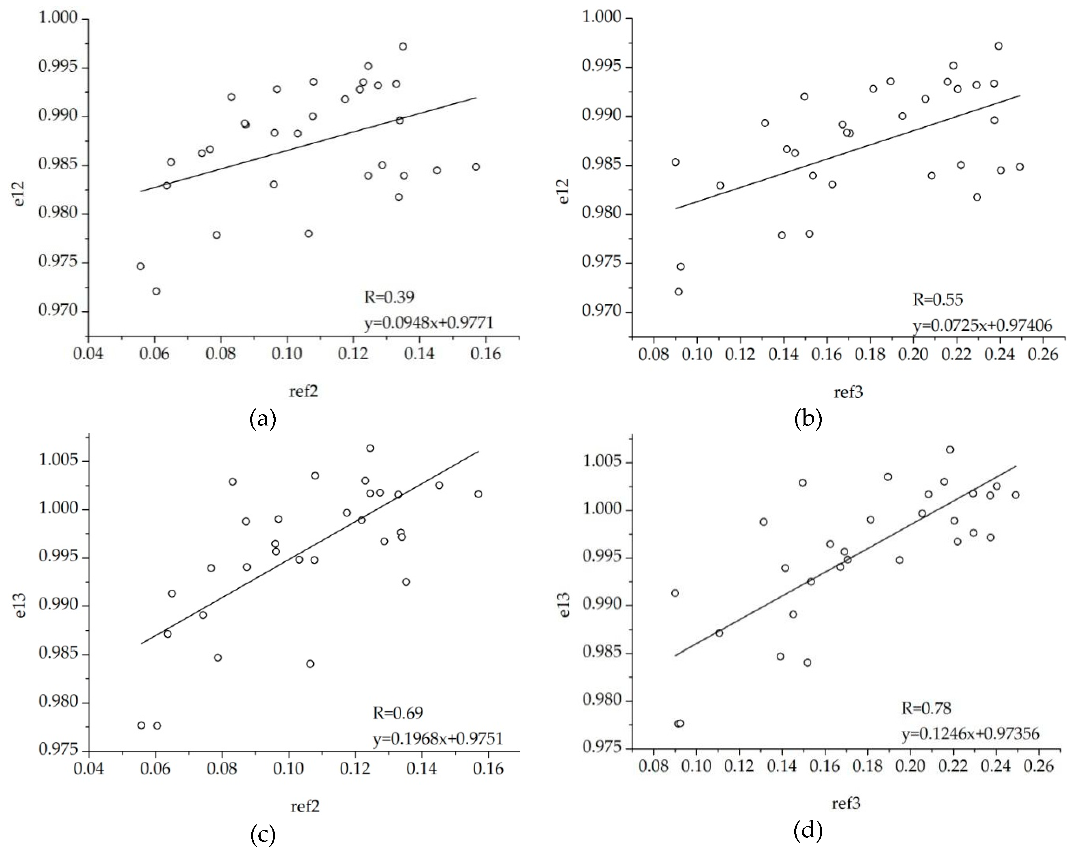
Two emissivity retrieval schemes were designed based on the emissivity model of Sobrino et al. The first scheme determines emissivity by estimating channel emissivity as shown in
Figure 4, which illustrates the correlation between the emissivity of the 12th and 13th channels of AGRI and the reflectance of its 2nd (red channel) and 3rd (near infrared channel) channels. Both e12 and e13 show a favorable correlation with ref2 and ref3, especially in terms of near infrared channel reflectance. Therefore, the new emissivity model of the 12th and 13th channels of AGRI was developed based on ref3. In
Figure 4b,d, the emissivity retrieved by this model is denoted by DX1.
Figure 4 also shows that despite the significant positive correlation between channel emissivity and reflectance, the scatters of e12, e13, and reflectance are relatively dispersed, thereby indicating potentially large deviations in the retrieved e12 and e13. Therefore, models that can directly retrieve average channel emissivity (referred to as e) and channel emissivity difference (referred to as de) were developed by using channel reflectance and its combined parameters, as shown in
Figure 5. The correlations between e and channel reflectance, and between de and channel reflectance, are all stronger than those between channel emissivity and channel reflectance. Moreover, e shows significant positive correlations with channel reflectance and its combined parameters, whereas de shows significant negative correlations with channel reflectance and its combined parameters. The correlation between de and NDVI, and that between e and “ref3–ref2”, are the most significant, with correlation coefficients reaching 0.86. The emissivity retrieved by this model is denoted by DX2.
2.2.3. PSO Algorithm
From the above local split-window algorithms, seven constant parameters in the B&L algorithm and six constant parameters in the Kerr algorithm need to be redefined based on specific regions and for FY-4A. In this paper, the artificial PSO was used to determine these parameters. PSO was implemented given its wide use in different fields [
39,
40]. The global optimal solutions of nonlinear algebraic equations can be obtained by constantly updating the combination of parameters, which minimizes the difference between observed and estimated values. The time needed for computation is less than that using the traditional iteration method.
The PSO was first proposed by Kennedy and Eberhart [
41] based on a study of the foraging behavior of birds. The PSO is a simple and effective spatial search method. This algorithm aims to find the minimum of the objective function in parameter space by updating the position and velocity of a group of random particle swarms. Supposing that n-dimensional problem is optimized to select m particles, the position and velocity functions of i particles can be respectively shown as follows:
The updated position and velocity of i particle are respectively computed as follows:
where po and v refer to position and velocity functions, respectively; Y denotes iterations; ω represents inertia weight; c
1 and c
2 correspond to acceleration constants; r
1 and r
2 are random numbers between 0 and 1; and L
i and G
n refer to the local and global optimal locations searched by i particles, respectively.
In this paper, the root mean square error (RMSE) was used as the objective function, and the solution corresponding to minimum RMSE during the iteration was taken as the optimal parameter. The PSO algorithm depends on parameters of the algorithm itself. These parameters include the number of particle swarms and variation range of position and velocity of particles. Based on a large number of simulation experiments [
42], the number of particle swarms is 200. Variation range of inertia weight is 0.2–0.5. Acceleration constant is 2.0. Variation range of particle position is −1.0–1.0, and that of particle velocity is −0.01–0.01. All parameters to be optimized were changed into an interval [−1.0, 1.0] unit by mapping:
where R
x refers to the value after parameter mapping; R
o denotes the actual parameter value; and R
max and R
min represent the actual maximum and minimum parameter values, respectively. In this paper, the maximum and minimum values of parameters were set to ±100 times of the parameter values used in the B&L algorithm.
2.2.4. Accuracy Evaluation of Estimation Results
In this paper, three statistics were used to evaluate estimation results:
(1) Root mean square error (RMSE)
(2) Mean absolute percent error (MAPE)
(3) Correlation coefficient (R)
where E
i refers to the estimate sequence;
represents the mean value of the estimate sequence; O
i denotes the measured sequence;
corresponds to the mean value of the measured sequence; and N denotes the number of samples participating in the calculation.
3. Results
To verify the applicability of the Kerr and B&L algorithms in Northwest China, the variables optimized by PSO are marked by “PSO”, whereas the variables in the original Kerr and B&L algorithms are left unmarked.
3.1. Diurnal Variation of Emissivity
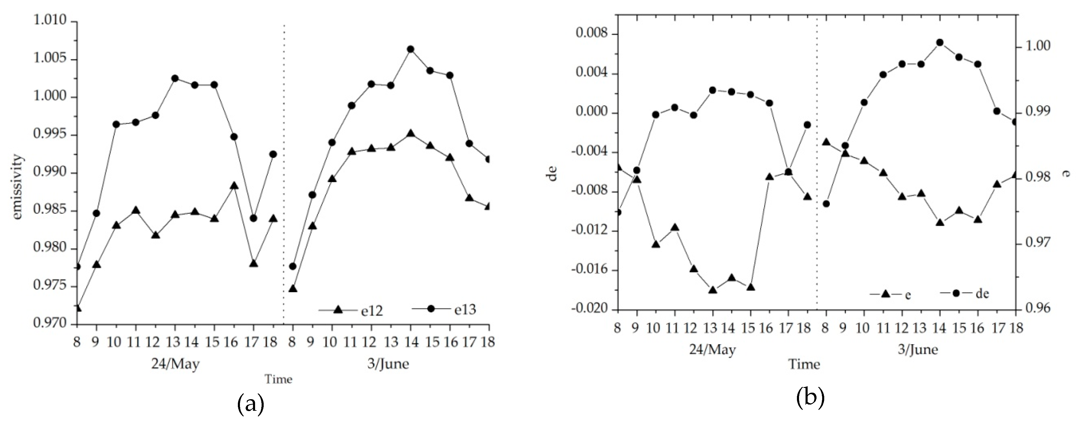
Figure 6 shows the diurnal variation of the measured emissivity for two typical sunny days from 08:00 to 18:00. In
Figure 6a, the e12 and e13, which correspond to the 12th and 13th channels of the AGRI, are between 0.97 to 0.99 and 0.97 to 1.005, respectively. Their diurnal amplitudes are 0.02 and 0.03 and their range of variation is small. However, the diurnal variations are obvious and reach their maximum values at noon.
Figure 6b shows the diurnal variation of the mean and difference of channel emissivity. The diurnal variation of channel emissivity difference is also obvious, but it reaches its minimum value at noon. When compared with the parameters of channel emissivity on 24 May and 3 June, the average emissivity of the two channels increases and the difference of emissivity decreases along with the growth of vegetation.
3.2. LST Retrieved by Local Split-Window Algorithms
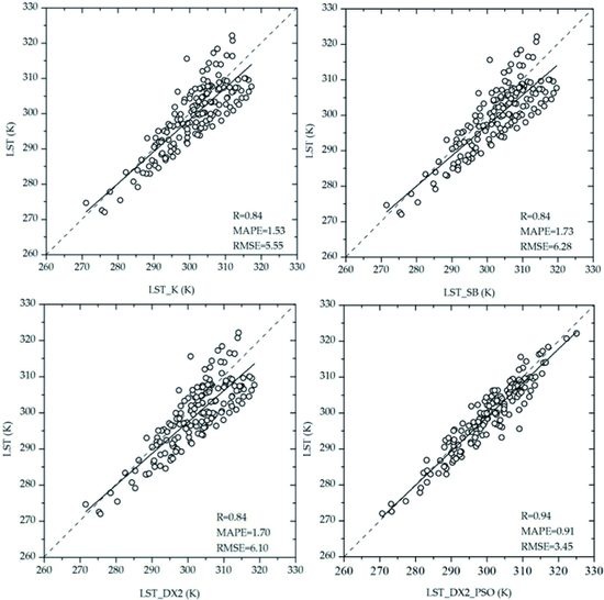
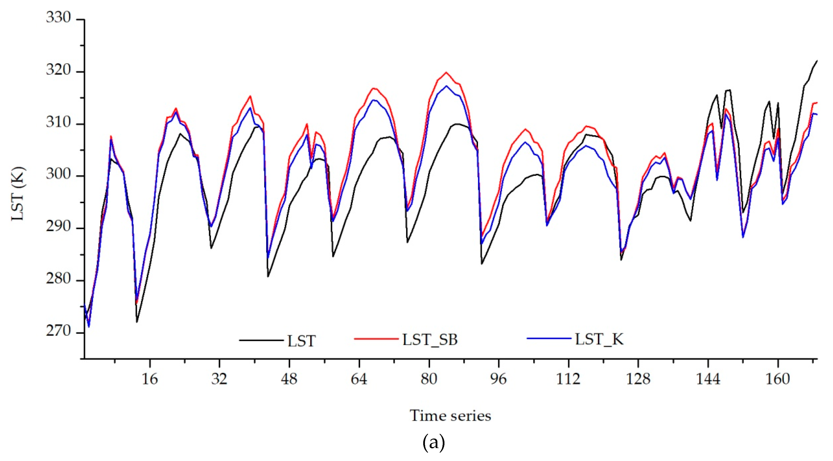
On the basis of FY-4A satellite data, the LSTs retrieved by different split-window algorithms and the measured values of various underlying surfaces in Northwest China are compared in
Figure 7. Given the large amount of precipitation in the summer of 2018 and 2019 in Gansu Province, the measured LSTs at all stations are all near 330 K. As shown in
Figure 7a, samples 1–123 were collected from the Dingxi station, samples 124–140 were collected from the Kangle station, and samples 141–169 were collected from the Qifeng station. The time series diagrams shown in this work are the same as
Figure 7a. Compared with the measured value, the LST retrieved by both the B&L and Kerr algorithms can reproduce the diurnal variation characteristics of LST. The correlation coefficients between the LST estimated by the split-window algorithms and the measured value all reached 0.84. However, the estimated LST of the two algorithms is higher than the measured value. In the low temperature region, the deviation between these two algorithms is small, and the estimated LST is close to the measured value. However, with an increasing LST, the deviation becomes greater (especially at noon), and the maximum deviation can reach approximately 10 K. The LST estimated by the Kerr algorithm is closer to the measured value than that estimated by the B&L algorithm. The RMSEs of the Kerr and B&L algorithms are 5.55 K and 6.28 K, respectively. From the analysis of different underlying surfaces, both split-window algorithms overestimate the LST of the vegetation underlying surface and underestimate the LST of the desert underlying surface.
3.3. Kerr Algorithm Optimization
The LST retrieved by the Kerr algorithm deviates from the measured value, especially in the high temperature region. In order to improve the accuracy of the estimated LST in Northwest China, the Kerr algorithm was directly optimized by PSO, while any other surface parameters, such as emissivity, were not included in the algorithm.
Figure 8 compares the LST estimated by the optimized Kerr algorithm with the measured value. Comparing this figure with
Figure 7c reveals that the PSO optimization cannot improve the accuracy of the LST estimated by the Kerr algorithm as a whole, and that the RMSE between the estimated LST and measured value is 5.84 K. Given the different underlying surfaces, as shown in
Figure 8a, when the vegetation of the Dingxi Station (i.e., before 13 May; samples 1–57 in the figure) and the Kangle Station (samples 124–140) is relatively low, the accuracy of the LST estimated by the Kerr algorithm is obviously improved after PSO optimization. In
Figure 8a, the blue line is closer to the black line (which denotes the time series of measured LST) than the red line (which denotes the time series of LST estimated by the Kerr algorithm before PSO optimization). In this case, with a higher LST, the improvements in the accuracy of the estimated LST becomes highly obvious. The vegetation of the Dingxi station is improved, along with the growth of wheat (that is, after 13 May; samples 58–123 in
Figure 8a), but such improvement significantly weakens the effect of PSO optimization. At the same time, the coefficients obtained by PSO on the vegetation underlying surface in the Dingxi station are not applicable to desert underlying surfaces as in the Qifeng station, where the deviation of the LST estimated by the optimized algorithm is larger than that of the LST estimated by the original Kerr algorithm. In sum, the Kerr algorithm has a simple calculation, and the LST estimated by the optimized Kerr algorithm on a sparse vegetation underlying surface is closer to the measured value than that before optimization.
3.4. B&L Algorithm Optimization
The accuracy of the LST estimated by the B&L algorithm is not only affected by the algorithm coefficients, but also by emissivity. Therefore, the influence of emissivity on the LST estimated by the B&L algorithm is discussed.
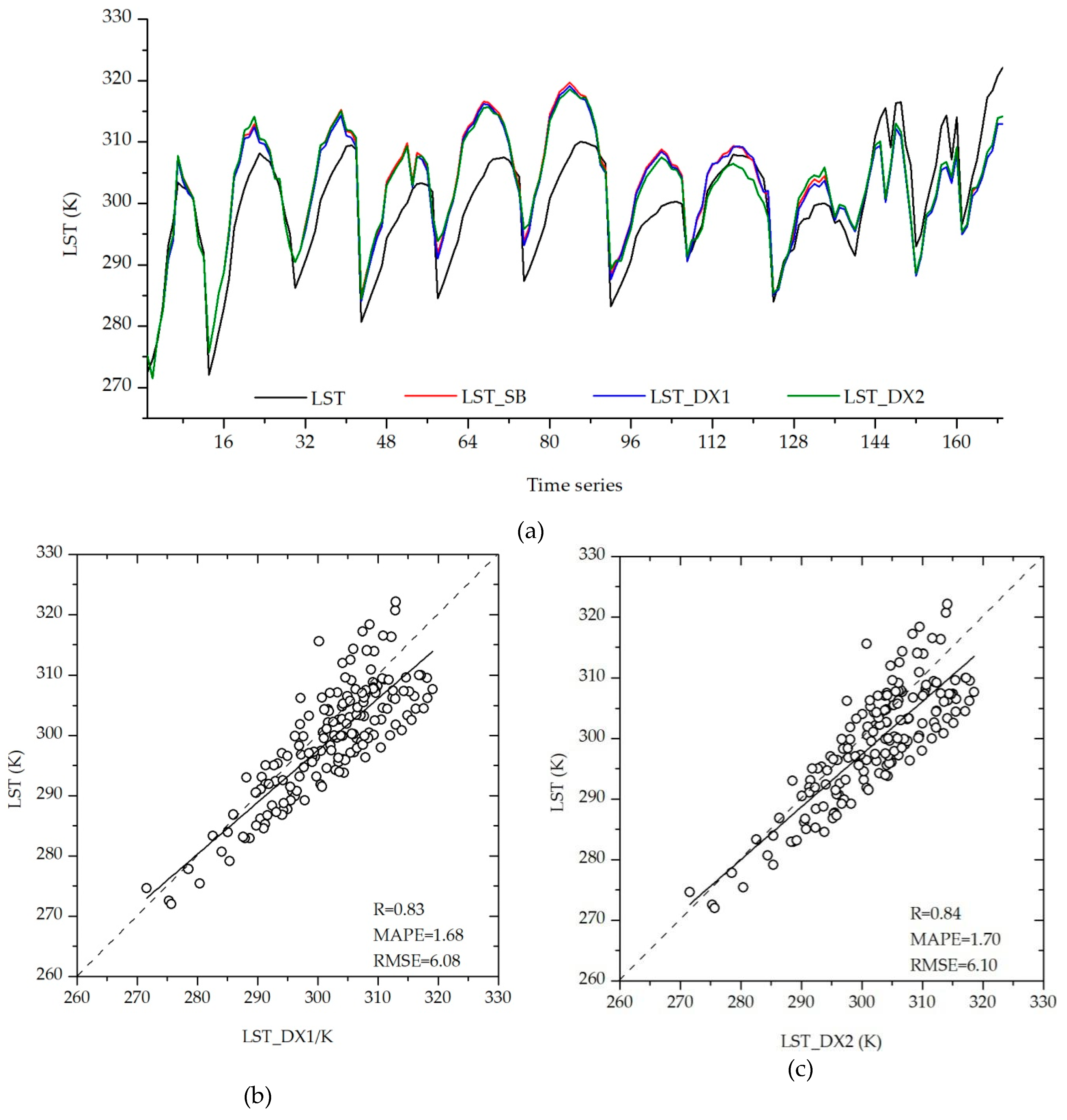
Figure 9 compares the observed value with the LST estimated by the B&L algorithm combined with different emissivity models. The variations in the LST estimated by the B&L algorithm combined with different emissivity models are in line with the measured values, and the correlation coefficients are all above 0.8. These numerical values all show that the LST estimation results deviate from the measured values. Comparing the LST estimated by different emissivity models reveals that the deviations among the LSTs estimated by the three emissivity models are small, and that the two new models developed by measured emissivity do not significantly reduce the retrieval error. The RMSE is only reduced by 0.2 K when using the new emissivity models for LST retrieval.
Given that the measured emissivity cannot significantly improve the accuracy of LST retrieval, one should consider whether the coefficients of the B&L algorithm are not optimal for the emissivity models. In this case, the PSO algorithm is applied to optimize the B&L algorithm. Given that both emissivity and LST are included in the B&L algorithm, the emissivity estimated by each model is assumed to be the “true emissivity” when the PSO is used to optimize the B&L algorithm. The coefficients in the B&L algorithm are then redefined based on this assumption.
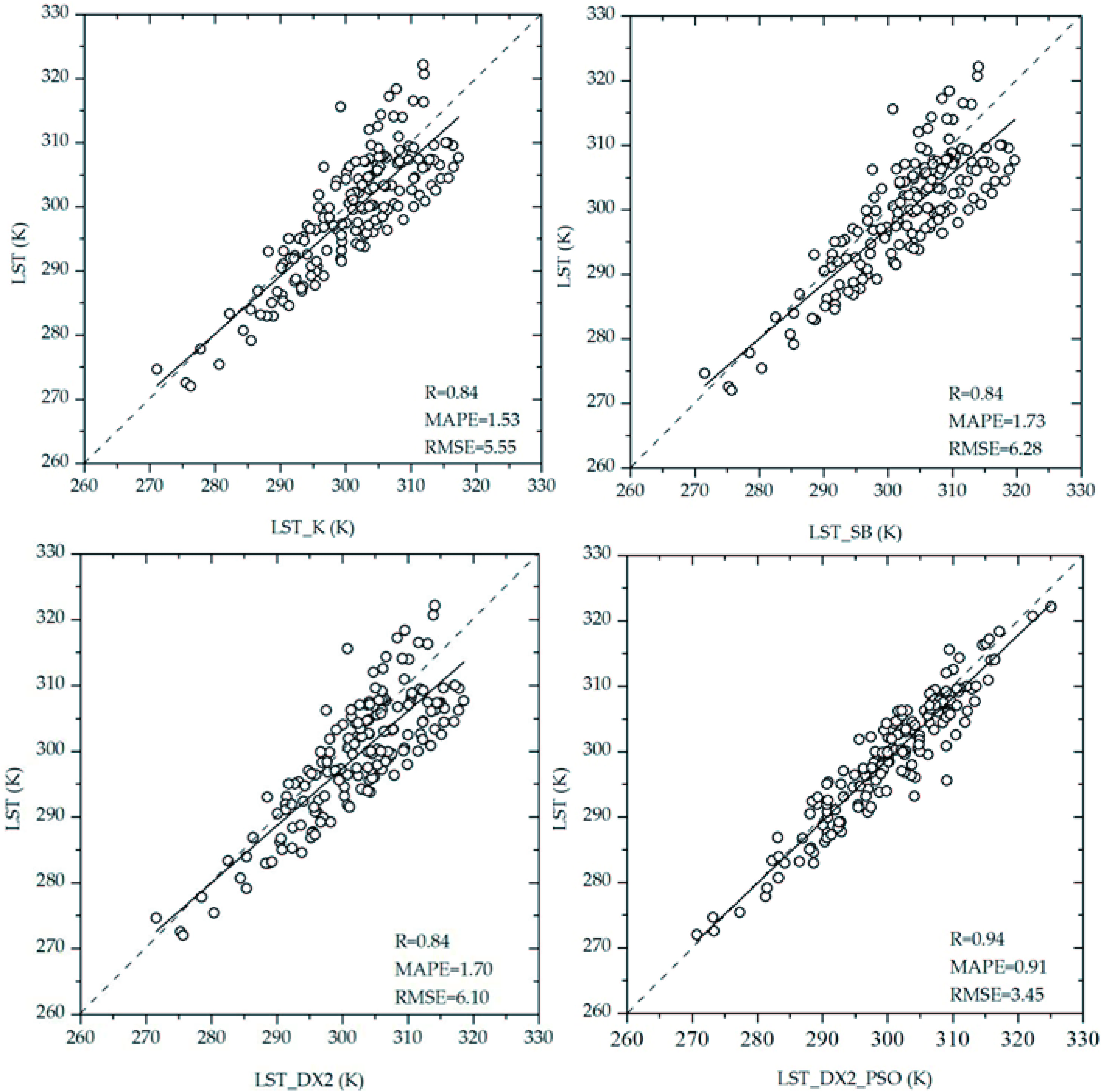
Figure 10b compares the observed value with the LST estimated by the B&L algorithm optimized based on the SB emissivity model. By comparing this figure with
Figure 7b, one can see that the estimated LST is closer to the measured value in the high temperature region, but the estimated LST is lower than the measured value in the low temperature region. Therefore, the LST estimated by the B&L algorithm optimized based on the SB emissivity model is not ideal, and the RMSE increases by 0.6 K after optimization, thereby suggesting that the original coefficients of the B&L algorithm are appropriate for the SB emissivity model and that local optimization cannot improve the retrieval accuracy of this algorithm.
Figure 10c compares the observed value with the LST estimated by the B&L algorithm that is optimized based on the DX1 emissivity model. By comparing this figure with
Figure 9b, one can see that the estimated LST is much closer to the measured value on the whole. The accuracy of LST retrieval is effectively improved by the local optimization of this algorithm, the RMSE decreases from 6.08 K to 4.84 K, and the error decreases by about 1.2 K via the local optimization of the algorithm. However,
Figure 10a shows that the LST estimated by the B&L algorithm that is optimized based on the DX1 emissivity model agrees with the measured values at the Dingxi (i.e., samples 1–123) and Kangle stations (i.e., samples 124–140). However, this LST is significantly lower than the measured value at the Qifeng station (i.e., the last 29 samples), and a huge deviation can be observed between the estimated LST and measured value. Therefore, for the measured emissivity, the coefficients of the B&L algorithm are no longer applicable. The accuracy of LST retrieval can be effectively improved via local optimization of the algorithm, but the DX1 model has poor universality. From the correlation analysis of channel emissivity and reflectance as shown in
Figure 5, both e12 and e13 are well correlated with the reflectance of the near-infrared channel. Therefore, the developed emissivity retrieval model is suitable for the vegetation underlying surface, such as the Dingxi and Kangle stations, and can estimate LSTs that are close to the measured values. However, the LST retrieval errors become larger when this model is extended to other underlying surfaces, such as the Qifeng station where the estimated LST is lower than the measured value.
Figure 10d compares the measured value with the LST estimated by the B&L algorithm that is optimized based on the DX2 emissivity model. By comparing this figure with
Figure 9c, one can see that the scatters between the estimated LST and the measured value are uniformly and closely distributed on both sides of the 1:1 line, the correlation coefficient increases from 0.84 to 0.91, and the RMSE decreases from 6.1 K to 3.45 K. The accuracy of the LST retrieval is therefore effective by the local optimization of the B&L algorithm. An analysis of
Figure 10a reveals that the emissivity model developed based on the differences in band reflectance is highly universal in Northwest China. The estimated LST of various underlying surfaces are all close to the measured values.
In sum, for the B&L algorithm, to obtain highly accurate LST retrieval results based on FY-4A satellite data, an improved emissivity retrieval model that is suitable for FY-4A must be developed. Comparing the LSTs retrieved by the two new emissivity models reveals that for the measured emissivity, the coefficients of the B&L algorithm are the main limiting factors for improving LST estimation accuracy based on FY-4A data. Therefore, to improve the accuracy of FY-4A LST retrieval, algorithm coefficients suitable for FY-4As satellites must be obtained via an algorithm optimization based on measured emissivity.
4. Discussion
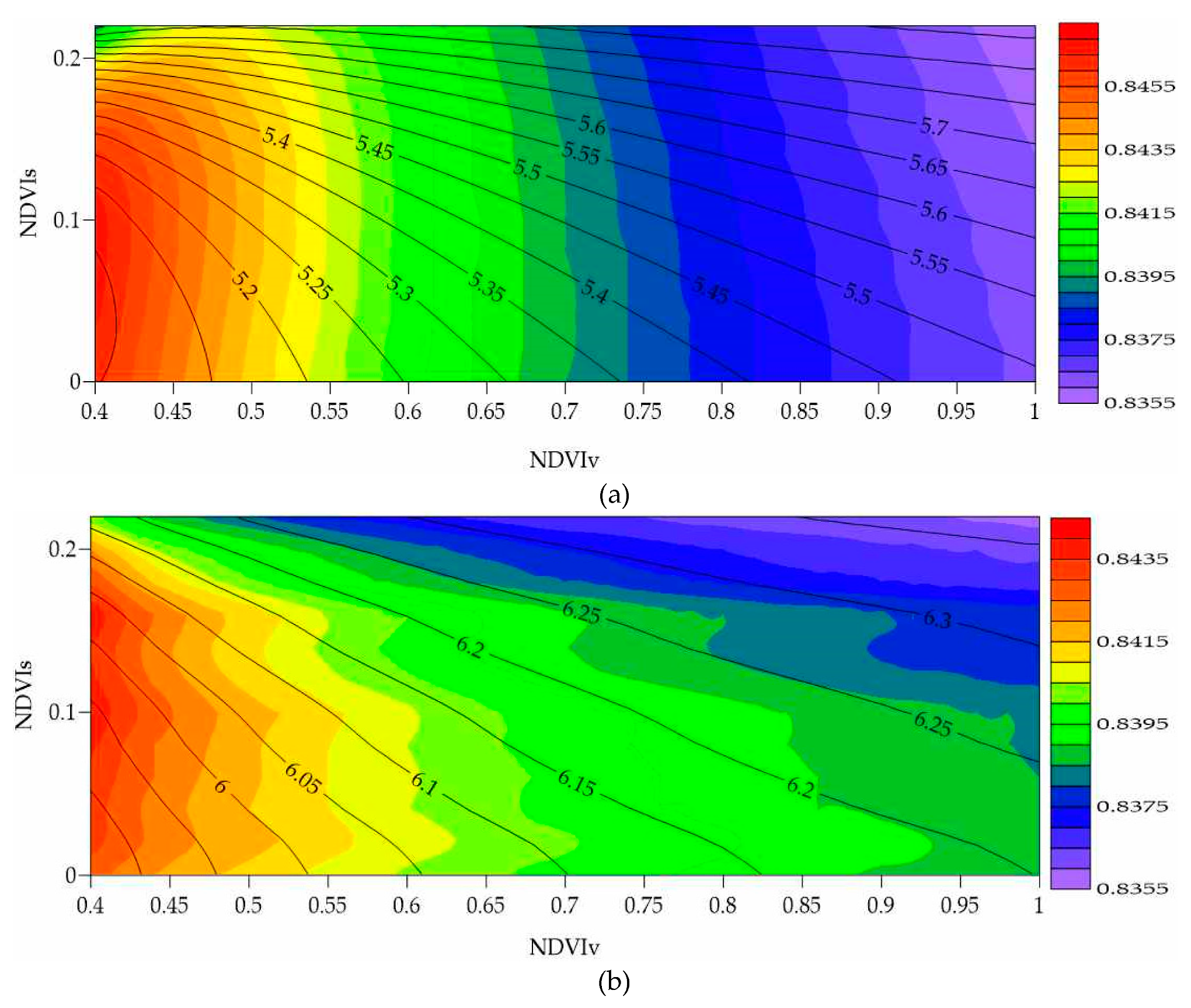
The results show that the Kerr algorithm only involves the calculation of vegetation coverage, while the calculation of vegetation coverage involves the determination of NDVIv and NDVIs. The differences in the LSTs estimated by the Kerr algorithm resulting from the changes in NDVIv and NDVIs are shown in
Figure 11. Based on FY-4A data, a smaller NDVI corresponds to a higher correlation and a smaller RMSE between the LST estimated by the Kerr algorithm and the measured value. By contrast, a larger NDVIv value corresponds to a smaller correlation coefficient and a larger RMSE between the LST estimated by the Kerr algorithm and the measured value in Northwest China. With increasing NDVIs, the color change becomes more obvious and the contour distribution becomes denser, especially at NDVIs values of above 0.2. In other words, with increasing NDVIs, the gradient of the correlation coefficient and the RMSE between the LST estimated by the Kerr algorithm and the measured value obviously increases. Given that the results of the B&L algorithm are similar to those of the Kerr algorithm, these results will not be discussed in detail. In sum, for retrieving LSTs in Northern China using FY-4A satellite data, the NDVIs and NDVIv should not exceed 0.12 and 0.5, respectively. In this way, the deviations in the RMSE resulting from the changes in the NDVIs and NDVIv values can be controlled within 0.1 K when the LST is estimated by the Kerr algorithm.
Given that the water vapor content products of FY-4A can be downloaded online from January 2019, the local split-window algorithm, which is related to water vapor, was not considered in this work. According to Quan, although the reflectance of 0.65 µm and 0.865 µm bands remains unchanged before and after atmospheric correction, the value of NDVI changes. However, the NDVI index is always used as a threshold parameter for classifying the underlying surface. Therefore, any change in NDVI will lead to different NDVI thresholds but will not greatly influence the accuracy of the LST estimated by the local split-window algorithm.
As can be observed from the LST estimated by the local split-window algorithm with optimized PSO, the original algorithm coefficients are identified as the optimal values for the local split-window algorithms after a long period of testing and improvement. Moreover, the accuracy of LST retrieval cannot be improved by algorithm optimization without changing any other parameter estimation model. To improve the LST retrieval accuracy, each parameter of the algorithm must be carefully estimated, and the coefficients of this algorithm must be redefined by using the artificial intelligence algorithm.
5. Conclusions
LST plays an important role in achieving energy balance. Therefore, accurately estimating the LST components is critical in studying land–atmosphere interaction and climate change. Remote sensing is the most convenient and effective means for obtaining regional-scale LST. Previous studies have shown that high-accuracy LST can be obtained by using the local split-window algorithm. Although a large number of local split-window algorithms have been developed to estimate LST for polar orbiting satellites, especially MODIS sensors, only few studies have attempted to develop algorithms for geostationary satellites. In 2016, China launched the FY-4A geostationary meteorological satellite, which can obtain high-resolution observational data. However, given the difference between FY-4A and polar orbiting satellites, the local split-window algorithm cannot be directly used for FY-4A. The data measured by FY-4A need to be revised and examined. The accuracy of the local split-window algorithm is verified based on the LST measured on different underlying surfaces in Northwest China. Meanwhile, on the basis of different emissivity models, the parameters of the B&L algorithm are optimized by using the artificial intelligence PSO algorithm. The major conclusions of this work are as follows:
(1) Based on FY-4A satellite data, the LST estimated by the Kerr and B&L algorithms can be used to reproduce diurnal variation characteristics. The estimated and measured values show a good correlation, but huge deviations can be observed in the estimated values. The correlation coefficients between the estimated LST and the measured value are all higher than 0.8, and the RMSEs of the Kerr and B&L algorithms are 5.55 K and 6.28 K, respectively. When the LST is high at noon, the deviation between the estimated and measured values increases. The estimated LST on the vegetation underlying surface is higher than the measured value, whereas the estimated LST on the desert underlying surface is lower than the measured value with a maximum deviation that can reach up to 10 K.
(2) The accuracy of the LST estimated by the optimized Kerr algorithm cannot be improved but can be influenced by the NDVIs and NDVIv values. For FY-4A satellite data, the NDVIs should not exceed 0.12 and NDVIv should not exceed 0.5 in Northwest China.
(3) The measured emissivity has obvious diurnal variation characteristics, but a small daily amplitude. The accuracy of the LST estimates retrieved by the B&L algorithm with measured emissivity also do not significantly improve.
(4) On the basis of different emissivity models, the B&L algorithm was optimized by the PSO algorithm, and the results show that the emissivity model and coefficients of the algorithm are two factors that limit LST retrieval accuracy. Only the optimal combination of these two factors can effectively improve the retrieval accuracy. According to the measured emissivity model, PSO can effectively reduce the deviation and improve the estimation accuracy, and the minimum RMSE of the LST estimated by the optimized B&L algorithm is 3.45 K.
This study is based on the idea that the FY-4A sensor is similar to the MODIS sensor in partial channel observations. Therefore, the B&L algorithm can be extended to FY-4A, and only a few empirical parameters need to be revised. As a new generation of geostationary satellite, FY-4A has its own characteristics in channel design, sensor response function, and satellite positioning. An important research task is to develop high-accuracy retrieval algorithms for the FY-4A satellite. Results of the present study show that, on the one hand, the existing split-window algorithms can be used for FY-4A. Combined with the advantages of the FY-4A satellite, such as the high-temporal-resolution observation data, the split-window algorithm can be applied to study diurnal variations of various variables, and the results could provide references for studies on diurnal variation characteristics of land surface variables or other parameters on regional and even larger scale. On the other hand, algorithm coefficients in the existing split-window algorithm and emissivity model cannot simply be used for FY-4A.


