1. Introduction
With the increasing complexity of the buildings in highly urban areas since the late 90s, 3D Cadastre has been a subject of interest. 3D Cadastre is beneficial for land registries, architects, surveyors, urban planners, engineers, real estate agencies, etc. [
1]. On one hand, it shows the spatial extent of the ownership and, on the other, it facilitates 3D property rights, restrictions, and responsibilities [
2,
3]. However, for realization of the 3D Cadastre concept, there is no one single solution. User needs, the national political and legal situation, and technical possibilities should be taken into account. This was also clear from the International Federation of Surveyors (FIG) questionnaire completed by many countries in 2010 [
4,
5]. In recent years, many 3D Cadastre activities have been initiated worldwide, since 3D information is essential for efficient land and property management [
6,
7,
8,
9]. An investigation into the legal foundation has been done for 15 countries covering Europe, North and Latin America, the Middle East, and Australia [
10], not only overground, but also underground [
11]. However, there is still no fully implemented 3D Cadastre in the world [
4] due to a lack of integration between legal, institutional, and technical parties involved. With the technical developments, physical and legal representation for the purposes of 3D Cadastre are being actively researched; however, considering the dynamics of the complex relationships between people and their properties, we must take into account the time aspect, which needs more attention [
12]. Most of the ongoing research on 3D Cadastre worldwide is focused on interrelations at the level of buildings and infrastructures. So far, the analysis of such interrelations in terms of indoor spaces, considering the time aspect, has not yet been explored. Therefore, the current paper aims to investigate the opportunities provided by automatic techniques for detecting changes based on point clouds in support of 3D indoor Cadastre. When using the term “automatic”, we mean that the process of change detection and separation of permanent changes from temporary changes are automatic. However, setting relevant parameters for each step is required by an expert. Moreover, Cadastral expert intervention is required to connect the land administration database, if it exists, to the physical space subdivision extracted from point clouds. The remainder of this section includes the relevance of our research, showing a real example in The Nederlands and related scientific work in the field.
In recent years, many examples can be found of changes in the functionality of buildings. According to the statistics shared by Rijksolverheid [
13] in The Netherlands, 17% of the commercial real estate is empty. The Ministry of Interior and Kingdom Relations (BZK) and the Association of Dutch Municipalities (VNG) set up an expert team to support municipalities in the transformation of empty buildings from commercial to residential use. One of the examples is a nursing home located in the city of Hoorn (
Figure 1a), 40% of which was owned by housing associations and 60% by health care organizations and was changed in 2015 into student accommodation and privately owned apartments (
Figure 1b).
From the recent research in the field, it was observed that point clouds are a valuable source for decision makers in the domain of urban planning and land administration. Laser scanner data acquired with aerial laser scanners (ALS), mobile laser scanners (MLS), and terrestrial laser scanners (TLS) have been used for reconstruction of 3D cities, building facades, roof reconstruction [
14,
15,
16], and damage assessment of the buildings before and after a disaster [
17]. In the domain of forestry, point clouds are used for monitoring the growth of trees and changes in the forest canopy. Xiao et al. [
18] used point clouds to monitor the changes of trees in urban canopies. Regarding buildings, some methods combine images with laser scanner data for facade reconstruction [
19,
20,
21]. There has been incredible progress in recent years in the automation of 3D modeling based on point clouds [
22,
23,
24] and more specifically in subdividing the space to semantic subdivisions, such as offices, corridors, staircases, and so forth [
25,
26,
27]. Challenges for detecting changes for updating 3D Cadastre in an urban environment using ALS and image-based point clouds for 3D Cadastre were also explored [
28]. Regarding indoor spaces, geometric changes during the lifetime of a building were analyzed for the Technical University of Munich (TUM) [
29], as shown in
Figure 2; however, they were not related to Cadastre. This fact motivates us to use point clouds and monitor changes for updating 3D Cadastre.
From a technical point of view, the three possibilities to detect geometric changes over time are:
Comparing two 3D models from two different epochs;
Comparing a 3D model with an external data source, e.g., point clouds, floor plans;
Comparing two point cloud datasets from two epochs to extract changes.
In the current paper, we are using the third option becausepoint clouds are used for change detection and representation of the 3D Cadastre because they reflect more detail of the environment and they are close to the current state of the building. Furthermore, it is easy to convert the point clouds to other data representation forms, such as vector and voxel, for usage in 3D Cadastre models [
30]. Having more than one point cloud dataset as an input information change detection can be done either in a low level of detail and just based on the geometry, or in a higher level of detail by interpretation of the geometry to semantics. The changes between two epochs could be due to differences in the furniture and not the permanent structure, which needs a higher level of interpretation from point clouds. However, only comparing the geometry of two point clouds is not sufficient to interpret 3D Cadastre related changes. Additionally, we need to have an understanding of the spaces inside the buildings to relate them to 3D spatial units in a 3D Cadastre model and properly register them in a database.
In the domain of Cadastre, there is a need to subdivide the spatial units vertically and have a 3D representation in 3D spatial databases. Van Oosterom discusses different types of data representation for 3D model storage. including voxels, vectors, and point clouds [
30]. The flexibility of point clouds in conversion to voxel or vector formats makes it easier to use point clouds in Cadastre. Additionally, point clouds can represent the 3D details of the buildings from inside and outside. From the standards and modelling aspects, researchers have developed models to provide a common framework for 3D Cadastre. The main international framework for 3D Cadastre is the Land Administration Model (LADM) [
31]. However, in LADM there is a lack of connection between spatial models, such as Building Information Models (BIM) and IndoorGML. Oldfield et al. [
32] try to fill this gap by enabling the registration of spatial units extracted from BIM into a land administration database. Aien et al. [
1] study the 3D Cadastre in relation to legal issues and their physical counterparts. The authors introduce a 3D Cadastral Data Model (3DCDM) to support the integration of physical objects linked with the legal objects into a 3D Cadastre. Another application of LADM is for using the access rights for indoor navigation purposes. The access rights of spatial units is defined in the LADM and could be connected to IndoorGML for customized navigation in the spatial units [
33]. Another model that builds on LADM for supporting the 3D spatial databases in terms of land administration was developed by Kalantari et al. [
34]. The authors propose strategies for the implementation of the 3D National Digital Cadastral Database (3D-NDCDB) in Malaysia. The proposed database gives instructions for cadastral data collection, updating the data and storage. Their database is a one-source 3D database which is compliant with the LADM. Other researchers discuss the need for new spatial representations and profiles (e.g., a point clouds profile for non-topological 3D parcels) [
35,
36]. Atazadeh et al. investigate the integration of legal and physical information based on international standards [
37].
It is challenging to automatically link the right spaces to the 3D Cadastre and database. For this task, each space subdivision can represent a spatial unit or a group of spatial units in a building. These spatial units, to some extent, are supported in LADM through four main classes: LA_Party, LA_RRR, LA_BAUnit, and LA_SpatialUnit [
38]. From the point of view of changes in indoor spaces LA_SpatialUnit, which represents legal objects, and LA_RRR, which represents rights, restrictions, and responsibilities, are the interesting classes. The reason that we decided to use the LADM for our experiments is that it is more complete and recent than other cadastral data models, such as the Federal Geographic Data Committee (FGDC) (Cadastral Data Content Standard—Federal Geographic Data Committee) [
39], DM01 [
40], and The Legal Property Object Model [
41]. Additionally, unlike other cadastral data models that are based on 2D land parcels, LADM suggests modeling classes for 3D objects [
1]. However, there is a lack of support for 3D Cadastre in terms of data representation and spatial operations in the current 3D Cadastre models, such as LADM. For example, Cadastre parcels are mainly represented as 2D parcels, while, in a multi-storey building, there is a need to show the property as a volumetric object. The only class for supporting 3D spatial units in the LADM is the Class LA_BoundaryFace, which uses GM_MultiSurface to model 3D objects. The problem of GM_MultiSurface is that it is not sufficient for 3D spatial analysis and representation [
1]. To compensate for this shortage in our workflow, enriched point clouds were used as an external database to store and represent the 3D objects. Using attributed point clouds enabled us to calculate necessary spatial attributes for 3D Cadastre.
Currently, there is no framework or standard for connecting point clouds, 3D models, and the LADM. Therefore, in this paper, we propose such workflow based on experiments on two different datasets. One example is of a commercial building, of which the point clouds are acquired using two different MLS systems before and after renovation. In addition, one more example of a building captured at different moments with TLS will be shown. This research shows the usage of point clouds as a primary and final format of data representation to enrich the 3D Cadastre. The remainder of this article explains the used methodology and the obtained results, followed by critical discussion and conclusions with a shared view on the way forward.
2. Materials and Methods
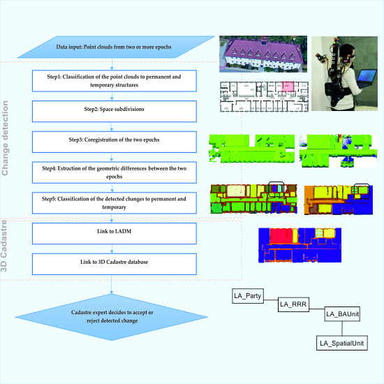
In the current section, the methods for detecting changes from point clouds and their possible links with LADM and the 3D database will be explained (
Figure 3). We set an external model between the attributed point clouds and LADM to execute 3D operations (e.g., to check the topology and calculate the area) on the point clouds and fed into the LADM. For understanding the changes, first, we classified the point clouds of each epoch to permanent (e.g., walls, floors, ceilings) and temporary structures (e.g., furniture, outliers) using the methods in [
42] (Step 1,
Figure 3). Second, space subdivisions, such as rooms, corridors, staircases, were extracted from the point clouds of each epoch (Step 2,
Figure 3). Two epochs were then co-registered and the geometric differences were extracted. The changes were classified as important changes, such as permanent structure and temporary changes, such as changes in the furniture (Step 3,
Figure 3). Furthermore, the relevant changes for 3D Cadastre were distinguished from other changes (Step 4,
Figure 3) and were connected to the space subdivisions. Each space subdivision represented a semantic space that was associated with the 3D Cadastre attributes (Step 5,
Figure 3). Finally, the related 3D Cadastre changes were queried from the database and a Cadastre expert decided the updating of the Cadastre records (
Figure 3).
2.1. Case Studies
For the current research, two case study examples are used. The first case study is the building of the Technical University in Braunschweig (TUB) and the second is the University of Twente Faculty of Geo-Information Science and Earth Observation (ITC) building. The floor plans of these buildings are shown in
Figure 4. In
Figure 4a, the highlighted area shows that a wall was removed and rooms were merged into one, and
Figure 4b shows the two rooms before removing the walls.
Point cloud data for the two case studies were collected with different scanners (
Figure 5). The data for the Braunschweig building were collected with an ITC Indoor Mobile Mapping System (ITC-IMMS) (epoch1) [
43] and a Zeb-Revo (epoch2) [
44]. For the ITC building, we used the Riegl [
45] terrestrial laser scanning system and a Viametris device. The accuracy of the point clouds varied from 0.01 to 0.06 m depending on the laser scanner system. While the noise in mobile mapping systems was louder than the terrestrial laser scanner (TLS), the scene coverage of a mobile mapping system was more than a TLS. The noise in the data could have been caused by sensors, data acquisition algorithms, and the reflective surfaces. For more information on the comparison of scanning systems, refer to the study by Lehtola et al. [
46].
In the following subsections, the detailed methodology is explained based on the first case study.
2.2. Indoor Change Detection from Point Clouds
Differences in two epochs of point clouds inside the buildings can be categorized as:
Changes in the dynamic objects (e.g., furniture);
Changes in the permanent structure (walls, floors, rooms).
There are some other differences between two epochs of point clouds that are interpreted as:
- 3.
Differences because of the acquisition coverage;
- 4.
Differences because of the difference in the sensors.
In our approach, categories number 1 and 2 were dealt with as important changes for 3D Cadastre, and categories 3 and 4 were just inevitable differences in two epochs that occurred because of data acquisition systems and were not relevant to the 3D Cadastre. We acquired two point clouds of two time periods with two different laser scanners, one a Zeb-Revo [
44] handheld MLS and the other an ITC-IMMS [
43]. The motivation to use different sensors is to explore all realistic possible causes of differences between epochs. The process of change detection starts with the co-registration of two point clouds (Step 3 from
Figure 3). The co-registration of two point cloud datasets was a straightforward approach, such as using the iterative closest point (ICP) [
47,
48,
49]. After the registration, two point clouds were compared based on the distance threshold to detect the differences caused by the registration error and sensors differences (4th category; Step 4 from
Figure 3). The distance threshold was chosen by summing the registration error and sensor noise. The registration error and sensor noise already introduced some differences between the two datasets. The registration errors were the residuals of each co-registration process (less than 10 cm). The sensor noise was specified in the specification of the systems. This threshold,
d, described points from two datasets with the distance less than the threshold. They were not considered as changes and they were in the 4th category because of the differences in the sensors. Points that had distances more than the threshold were in one of the other three categories. In our experiment, we defined the distance threshold of less than 0.10 m.
Let the point clouds (PC) from epoch one (acquired by a backpack) be PC1 and the point clouds from the second epoch (acquired by Zeb-Revo) be PC2. The point to point comparison was based on the reconstruction of a Kd-tree [
50,
51] and a comparison of the distance of the points in PC1 from PC2 and was stored in PC1. Using this method, the differences caused by the acquisition system and registration errors were excluded from the real changes.
In the next Step 5 from
Figure 3, the differences were further analyzed to detect and exclude the acquisition coverage (3rd category). Our change detection method was based on analyzing two geometric differences between two point clouds. This was done in two steps: (1) The distinction was made between object changes and coverage differences and (2) the object changes were separated into changes on permanent structures and dynamic objects, such as persons and furniture (
Section 2.2).
The geometric differences were calculated by determining the nearest 2D point and the nearest 3D point in the other epoch. The first nearest point was based on the X, Y coordinates and the second on X, Y, Z coordinates.
Figure 6 shows both geometric distances as a point attribute categorized in three colors: Green <20 cm, yellow >20 cm and <50 cm, red >50 cm to the nearest.
For both object changes and coverage differences, it was expected that the nearest 3D point was further than a certain threshold. However, the nearest 2D point may have been close to a changed object, but not in case of coverage differences. Points were temporarily labeled as part of changed objects if the distance to the nearest point in 3D was larger than 20 cm, but the nearest point in 2D was less than 20 cm. Threshold values were chosen such that they were larger than the expected registration errors but small enough to detect changes larger than 20 cm. Next, the whole point cloud was segmented into planar segments and only the vertical segments with a majority (more than 50%) of points labeled as potentially changed were considered to be changed. The planar segmentation was performed by a region growing algorithm presented by Vosselman et al., [
52]. Note that, in this way, the points on a newly built wall near the ground or ceiling, with a small 3D distance to the nearest point in the other epoch, were included in the changed objects as they belonged to a segment with more than 50% points with a large perpendicular distance to the plane in the other epoch. By using planar segments and calculating perpendicular distances from a point in one epoch to a plane in the other epoch, we avoided the influence of differences in point densities between the point clouds. The vertical segments labeled as changed objects included permanent structures, such as walls, but also dynamic objects, such as persons. In the second step, the aim was to separate permanent from temporary changes by looking at a method described in [
23] and [
42].
2.2.1. Classify Changes to Permanent and Non-Permanent
The next step was to separate the changes that were part of the permanent structure from dynamic objects. This involved classifying the point clouds in each epoch to a permanent structure (e.g., walls, floors, ceilings) and a non-permanent structure (e.g., furniture, clutter and outliers).
In
Figure 7c, the blue color represents the areas captured by Zeb-Revo and the red areas show the differences in the coverage where PC1 is not covered by PC2. In
Figure 7d, the point clouds of epoch1 after the comparison with the epoch2 are shown and the blue points show the points in which their distance differences are less than the threshold and are not changed. The green points show the changes, because of coverage or furniture, or a permanent change, and the ceiling is removed for better visualization. We applied a method from [
23] to classify the permanent structures in each epoch (see
Figure 8). Four main classes were important for our change detection process. Walls, floors, and ceilings were three classes that belonged to the permanent structures. The non-permanent structures were, for example, furniture, outliers, and unknown points, which were classified as the clutter. The classification started with surface growing segmentation and generating an adjacency graph from the connected segments. By analyzing the adjacency graph, it was possible to separate permanent structures, such as walls, because of their connection to the floor and ceiling. The normal angle of the planes was important in this decision because walls in most indoor environments have an angle of more than 45 degrees with the positive direction of the
z-axis.
Figure 8c shows that the permanent structure (walls and floor) was separated from the clutter.
After the classification of points in each epoch, by comparing the changes with the semantic labels (walls, floors, and ceilings), it is possible to distinguish relevant changes for 3D Cadastre. Each point in the set of changes is a possible change for 3D Cadastre if is labeled as a wall, floor, or ceiling, otherwise it is a change only because of furniture or dynamic objects or outliers.
Table 1 shows how we identified changes with labels per point, respecting the permanent structure. According to the table, points with label 1 are important for change detection in 3D Cadastre because they represent a permanent change in the building.
Figure 5 represents the changes with different colors according to their label.
2.2.2. Changes in Relation to Indoor Space Subdivisions
The process of detection of permanent changes is continued by linking detected changes to the volumetric space or space subdivisions. Space subdivisions represent the semantic space in an indoor environment, such as offices, corridors, parking areas, staircases, and so forth. Each space subdivision is connected to space in a spatial unit in the 3D Cadastre model and all laser points in the space subdivisions carry the attributes of the corresponding Cadastre administration. In this step, we explain how these space subdivisions were extracted from the point clouds and linked to the previously detected changes. Note that an apartment may consist of one or more spatial units, a spatial unit may consist of one or more spaces, and a spatial unit may have invisible boundaries and needs to be checked by a Cadastre expert.
Following the method in [
23], after the extraction of the permanent structures in each epoch, a voxel grid was reconstructed from the point clouds, including walls, floors, and ceilings. Using a 3D morphology operation on the voxel grid, space was then subdivided into rooms and corridors. Each space subdivision was represented with the center of voxels as a point cloud segment. To find out which changes occured in which space subdivisions, we intersected the space subdivisions of each epoch with the permanent changes detected earlier (see
Figure 9). For example, in
Figure 8, we can see that in the second epoch (
Figure 8b) a wall was removed and two spaces were merged. Since this wall was detected as a change during the previous step (
Figure 8c) by the intersection of changed objects with subdivisions, the changes in the two epochs were extracted (
Figure 9). These changes were linked to a space subdivision, and each space subdivision or a group of them (e.g., a building level) may represent a spatial unit in the 3D Cadastre model.
2.2.3. Changes in Relation to the 3D Cadastre Model
To link the Cadastre to the detected changes, we assumed that every space subdivision in the point clouds was represented in the object description of the spatial unit in the LADM, considering that an interactive refinement on the space subdivision from the previous step was necessary to group some of the subdivisions, according to the 3D Cadastre legal spatial units. For example, a group of offices that belonged to the same owner had an invisible boundary that should be interactively corrected. LADM represents legal spaces in spatial units. Spatial units were refined into two specializations [
38].
- (1)
Building units, as instances of class:
LA_LegalSpaceBuildingUnit. A building unit concerns the legal space, which does not necessarily coincide with the physical space of a building. A building unit is a component of the building (the legal, recorded, or informal space of the physical entity). A building unit may be used for different purposes (e.g., living or commercial) or it can be under construction. An example of a building unit is a space in a building, an apartment, a garage, a parking space, or a laundry space.
- (2)
Utility networks, as instances of a class:
LA_LegalSpaceUtilityNetwork. A utility network concerns legal space, which does not necessarily coincide with the physical space of a utility network.
The LADM class LA_BAUnit (
Figure 10) allowed the association of one right to a combination of spatial units (e.g., an apartment and a parking place).
A basic administrative unit (LA_BAUnit) in LADM is an administrative entity, subject to registration, consisting of 0 or more spatial units, against which (one or more) homogeneous and unique rights (e.g., ownership right or land use right), responsibilities, or restrictions are associated to the whole entity, as included in a land administration system. In LADM, each space is represented as a spatial unit and then uses a LADM class LA_BAUnit to associate those spatial units to a legal unit. The type of building units were individual or shared. An individual building unit is an apartment and represents a legal space. A building contains individual units (apartments), a shared unit with a common threshold (entrance), and a ground parcel. Each unit owner holds a share in the shared unit and the ground parcel.
Every spatial unit in LADM was modelled with GM_MultiSurface. 2D parcels were modelled by boundary face string (LA_BoundaryFace). The representation of 3D spatial units was done by boundary face (LA_BoundaryFace), and for the storage a GM_Surface was used (see
Figure 11). However, in our approach, we are aiming to keep the point clouds until the last step for spatial analysis. Therefore, we just used the calculated features, such as volume, area, and neighboring units, to insert them as classes in the LADM. All spatial attributes and legal issues, such as rights, restrictions, and responsibilities, could be associated between point clouds and LADM. The measured spaces were important because, apart from the floor space, the volumes are also known. This is relevant for valuation purposes of the individual spaces in apartments.
Figure 12 illustrates the LADM representation of an apartment—in this case, owned by a party (right holder) named Frank. This party has an individual space and a share (1/100) in the common or shared space. Individual and shared spaces (including the ground parcel) compose the building as a whole.
The limiting factor of associating detected space changes to the LADM is that the LADM only provides an abstract representation of 3D objects with no direct mapping to an implementation. There are also specialized data structures, such as CityGML or IndoorGML, which can be used to store 3D data as specified in the LADM model. The issue here is that these data structures are primarily designed for visualization and indoor navigation and not for the management of rights of legal spaces. This becomes more apparent when looking at the definition of primal and dual spaces. The primal space is used to represent semantic subdivisions (e.g., a room, a corridor) and the dual space is used to represent the navigability of the primal space. For the proper management of legal space in a database and to properly determine which changes in the layout of a building affect legal spaces, additional information is needed to be stored in the database, namely, a direct relationship between visible and invisible subdivisions of space and the legal objects in the 3D Cadastre.
Given today’s database technology, the available option for the implementation of 3D legal spaces and their corresponding topological relationships is a GM_PolyhedralSurface [
53]. A PolyhedralSurface datatype is defined as a collection of polygons connected by edges which may enclose a solid. When using such a data structure, it is possible to define a subdivision in a building as the primal space and a legal object as the dual space. This way, properties can be assigned to, for example, walls to define whether it corresponds to a legal boundary or not (or where in the wall the boundary is). Similarly, properties can be assigned to invisible space subdivisions that define a change in the rights of the spaces. In this scenario, the dual of an edge is a face and the dual of a face is solid, which will represent a LA_BAUnit. A database implementation of the topological relationships of a PolyhedralSurface as required by a 3D Cadastre can be based on dual half-edges [
54,
55]. With this approach, each face is stored as an array of half-edges and can be associated with a set of attributes. These attributes can be defined as a result of the face detection from the point-cloud analysis. Since each face is associated to a legal object, it is possible to support the update of the 3D Cadastre by directly updating changes detected in the latest point cloud epoch on the database structure of the 3D Cadastre. This has to be followed by an update on the rights of the legal objects which will require the intervention of the cadastral expert responsible for mutations and transaction in the land administration system.
3. Results and Discussion
The proposed method is tested on two datasets. One dataset has a smaller amount of clutter and the shape of the building has a regular structure. Therefore, the separation of walls is easier. To challenge the robustness of our method with a complex structure and more furniture, a dataset with arbitrary wall layout and glass surfaces is selected (ITC restaurant,
Figure 12). The details of the datasets for each epoch are in
Table 2.
First, the datasets from two different epochs were co-registered using the iterative closest point ICP algorithm (
Figure 13). Then the changes between two epochs were identified in 2D and 3D, as explained in the methodology (
Section 2.2). The classification algorithm separated the permanent changes from non-permanent changes and then we intersected the permanent changes with the reconstructed spaces from two epochs (
Figure 14 and
Figure 15). In this way, the changes in the rooms in the second epoch of both datasets can automatically be identified. To identify the relation of physical changes with the 3D Cadastre, a user adds the ownership of the spaces as an attribute to each space. For example, the spaces which have the same rights and ownership obtain the same label and form a new physical space (
Figure 16). Then it is possible to connect them to the basic class of the LA_Spatial Unit in the LADM and update the spatial unit class in the LADM.
In dataset 2 (ITC restaurant), part of the curtain was identified as the permanent change because the curtains were covering the walls and they were detected as a permanent structure. However, this can be the inaccuracy of the classification method, for identifying the changes in the space is not problematic because it has a slight change in the space partitioning.
The important parameter for the detection of changes is the distance threshold (d) to identify the changes from the differences caused by noise and registration errors. We set this parameter slightly larger than the sum up of the sensor noise coming from the scanning device and the residuals coming from the ICP algorithm (less than 10 cm). In our experiments, we set this threshold on 20 cm, which implies that we cannot detect changes which are smaller than 20 cm. For planar segmentation of the point clouds, the smoothness parameter for a surface growing algorithm is important, which depends on the noise and point spacing in the data. We set the smoothness threshold to 8 cm because the noise from MLS systems (Viametris and Zeb-Revo) is around 5 cm. The smoothness parameter was set slightly larger than the sensor noise and point spacing. The point spacing was 5 cm, which meant we could subsample point clouds to reach 5 cm point spacing. The parameters for detecting the permanent structure were chosen according to [
23]. Segments with more than 500 supporting points were selected for creating the adjacency graph and smaller segments were discarded. The voxel size for space partitioning was 10 cm, which is an apppriate voxel size to have enough precision to identify changes and avoid expensive computations.
The running time for surface growing segmentation, identifying the permanent structure, and detecting the changes for the first dataset with 1.7 million points took 2.4 min, 5.6 min, and 7 min, respectively. The space partitioning was computationally more expensive than other processes and it took 10 min for dataset 1 with the voxel size of 10 cm, and it depended on the volume of the building. Larger volumes required more voxels for morphological space partitioning.
In our workflow, the challenge was detecting the permanent changes from the dynamic changes, which were not important for the Cadastre. According to [
23], this process can have an average accuracy of 93% for permanent structures and 90% for spaces [
57]. Furthermore, the extraction of spaces are really crucial in the process, because the volume and area is calculated from the space subdivision result. Therefore, an expert should check the results of space subdivision and merge or split some of the spaces that are extracted from the point clouds. The interactive corrections are less than 10% of the whole process and, for a building of three floors as large as our case study, it does not take more than 10 min.
The process of linking the spatial units to the 3D Cadastre model was not automated in our approach. This was because of the lack of possibilities for representation and visualization of 3D objects in the 3D Cadastre models. Therefore, our method was limited when it comes to the storage of 3D spatial objects in the Cadastre databases. As future work, linking the 3D objects and 3D Cadastre models, one solution we intend to investigate is using the point clouds as external classes and trying to keep the 3D objects as point clouds for all steps. The extraction of vector boundaries for the Cadastre models can be done with functions from the point clouds.

 ,
, 


