Article

A Modeling and Measurement Approach for the Uncertainty of Features Extracted from Remote Sensing Images

1
School of Remote Sensing and Information Engineering, Wuhan University, Wuhan 430079, China
2
State Key Laboratory of Information Engineering in Surveying, Mapping and Remote Sensing, Wuhan University, Wuhan 430079, China
*
Author to whom correspondence should be addressed.
Remote Sens. 2019, 11(16), 1841; https://doi.org/10.3390/rs11161841
Submission received: 9 July 2019 / Revised: 2 August 2019 / Accepted: 6 August 2019 / Published: 7 August 2019

Abstract

:
The reliability of remote sensing (RS) image classification is crucial for applying RS image classification results. However, it has received minimal attention, especially the uncertainty of features extracted from RS images. The uncertainty of image features constantly accumulates, propagates, and ultimately affects the reliability and accuracy of image classification results. Thus, research on the quantitative modeling and measurement of the feature uncertainty of RS images is very necessary. To make up for the lack of research on quantitative modeling and measurement of uncertainty of image features, this study first investigates and summarizes the appearance characteristics of the feature uncertainty of RS images in geospatial and feature space domains based on the source and formation mechanisms of feature uncertainty. Then, a modeling and measurement approach for the uncertainty of image features is proposed on the basis of these characteristics. In this approach, a new Local Adaptive Multi-Feature Weighting Method based on Information Entropy and the Local Distribution Density of Points is proposed to model and measure the feature uncertainty of an image in the geospatial and feature space domains. In addition, a feature uncertainty index is also constructed to comprehensively describe and quantify the feature uncertainty, which can also be used to refine the classification map to improve its accuracy. Finally, we propose two effectiveness verification schemes in two perspectives, namely, statistical analysis and image classification, to verify the validity of the proposed approach. Experimental results on two real RS images confirm the validity of the proposed approach. Our study on the feature uncertainty of images may contribute to the development of uncertainty control methods or reliable classification schemes for RS images.

Graphical Abstract

1. Introduction

With the continuous development of space-to-earth observation technology, increasingly different types of remote sensing (RS) imagery have been developed, and the spatial and temporal resolutions of RS imagery have increased. Accordingly, many types of image classification methods have been proposed. These methods include maximum likelihood classification [1], support vector machine (SVM) [2,3], random forest [4], rotation forest [5], object-oriented image classification methods [6,7,8,9,10], and deep learning-based classification methods [11,12]. However, the results of image classification still cannot achieve 100% accuracy or a sufficiently convincing level of accuracy and sufficient reliability despite significant progress in the field of RS image classification. Thus, RS image classification remains a problem that must be solved [13].
Uncertainty propagation theory [14,15] states that uncertainties are present in every stage of RS image classification. These uncertainties constantly propagate and accumulate during classification and ultimately affect the accuracy and reliability of the classification results. To achieve further breakthroughs in the field of image classification, we must systematically investigate the uncertainties in image classification [16,17] because they are the root cause of the reduction in the reliability of image classification results. Furthermore, these uncertainties inevitably cause errors in classification results and significantly limit the improvement of the accuracy and reliability of current image classification.
At present, numerous studies have been conducted on RS image classification, but studies on the reliability or uncertainty of RS image classification have received relatively minimal attention. Wilson and Granlund [18] proposed that uncertainty is a fundamental result in signal processing, and its impact must be considered throughout the entire image processing pipeline. Carmel [19] introduced an aggregation-based uncertainty control method for RS data. Li and Zhang [20] presented a Markov chain geostatistical framework for land cover classification. This model can provide an uncertainty assessment of the classified data. Gillmann et al. [21] proposed that the main source of data uncertainty was the data acquisition process itself, and additional uncertainty would be introduced during data processing. Gillmann et al. [22] also proposed an uncertainty-aware image pre-processing paradigm, which considered the input image’s uncertainty and propagated it through the entire pipeline. Giacco et al. [23] demonstrated the importance of uncertainty measurement in fusing several classifiers by analyzing the uncertainty in multispectral image classification using SVMs and self-organizing maps. Hughes and Hase [15] presented a practical guide for uncertainty/error analysis of measurements. This guideline describes some rules for uncertainty propagation. Feizizadeh [24] developed an approach for accuracy assessment and spatial uncertainty analysis in object-based image classification. This approach integrates fuzzy synthetic evaluation and the Dempster–Shafer theory. Gillmann et al. [25] considered the uncertainty of image segmentation and presented a flexible multiclass segmentation method, which fuses a fuzzy and a hierarchical segmentation approach to obtain an efficient segmentation result. Moreover, the uncertainty of the segmentation result was visualized. Shi et al. [26] designed a validation scheme for the reliability evaluation of results and processes of land cover classification to evaluate the reliability of land cover products. However, most existing studies on the uncertainty/reliability of RS image classification have focused on evaluating the reliability/uncertainty of classification results or improving the reliability of classification results by controlling uncertainty. The uncertainties in each stage of image classification have been rarely investigated and quantitatively described.
The uncertainty in image classification limits the reliability and accuracy of image classification results. To overcome this limitation, we must first understand the characteristics of the uncertainty in image classification and quantitatively measure and model it accordingly. Subsequently, we can control or constrain the uncertainty to reduce its negative impact on the image classification results and thus improve the reliability and accuracy of image classification. Feature extraction is a crucial stage of image classification, and the features constructed by feature extraction are the basis and premise of image classification [27,28,29,30]. Therefore, the uncertainties in image classification, especially the uncertainty of features extracted from RS images, must be quantitatively described and modeled.
However, as mentioned previously, to date, few relevant studies or methods have been proposed to model and measure the uncertainty of features of RS images in existing studies on uncertainty. To make up for this deficiency, this study focuses on quantitatively modeling and measuring the uncertainty of image features and proposes an effective modeling and measurement approach. Moreover, this study is expected to provide a basis for studying the accumulation and propagation mechanisms of uncertainty in RS image classification and guidance for studying RS image uncertainty control methods, which will contribute to improving the accuracy and reliability of RS image classification. Note that the feature uncertainty here mainly refers to classification uncertainty/confusion caused by mutual interference and confusion between features of different classes in the image due to adjacency effects, intra-class differences, and inter-class similarities, etc. The uncertainties caused by other factors, such as the accuracy of radiation correction, the representativeness of the selected samples, and the robustness of the classification algorithm, are not investigated in this study.
To achieve the modeling and quantification of the uncertainty of image features, the characteristics of feature uncertainty are first systematically investigated and summarized in this study from the perspectives of geospatial and feature space domains. The formation of the topic on the classification uncertainty of image features is one of the innovations of this study. Then, to make up for the lack of research on quantitative modeling and measurement of uncertainty of features extracted from RS images, this study proposes a modeling and measurement approach for quantifying uncertainty of image features. In this approach, a Local Adaptive Multi-Feature Weighting Method based on Information Entropy is proposed to model and measure the feature uncertainty of the image in the geospatial domain; and the Local Distribution Density of Points (LDDP) is proposed to model and measure the feature uncertainty in the feature space domain. In addition, a new feature uncertainty index is also constructed to comprehensively describe and quantify the feature uncertainty. The constructed feature uncertainty modeling approach (including the proposed index FUI) is one of the main contributions of this study. Finally, to verify the validity of the proposed approach, two different verification schemes are also proposed from two perspectives, namely, statistical analysis and image classification. These perspectives can prove the validity of the proposed approach and its practical value in image classification. Moreover, the proposed verification schemes will be useful for the validation of uncertainty quantification results of other stages of image classification in the future. It should be noted that this paper is different from our previous work [31], which proposes an uncertainty descriptor to quantify the effect of image quality itself on image classification results.
The remaining parts of this paper are organized as follows. Section 2 conducts a characteristic analysis of the feature uncertainty of RS images based on geospatial and feature space domains. Section 3 presents an approach for modeling and quantifying the feature uncertainties analyzed in Section 2 and constructs a feature uncertainty index (FUI). Section 4 designs two validity verification schemes for the proposed modeling and measurement approach. After that, Section 5 describes the experimental results and analysis on two test RS images and discusses the sensitivity of the parameters in the proposed approach. Finally, Section 6 draws the conclusions of this paper.

2. Characteristic Analysis of Feature Uncertainty

A crucial step before classifying an RS image X is to extract a series of features from an image (such as spectral and texture features). This process is the basis for image classification. Let the total dimension of the features extracted from image X be n. Evidently, due to the effects of image noise, mixed pixels, and the phenomenon wherein the same objects have different spectra or the different objects have the same spectra, the extracted n-dimensional features for different pixels in the image typically contain different degrees of uncertainty. The various degrees of uncertainty cause inevitable classification confusion among different categories of pixels when performing image classification. This uncertainty of features makes different pixels have distinct distribution or appearance characteristics in the image. Next, the distribution or appearance characteristics of pixels with different degrees of feature uncertainty are analyzed in detail from the perspectives of geospatial and feature space domains.

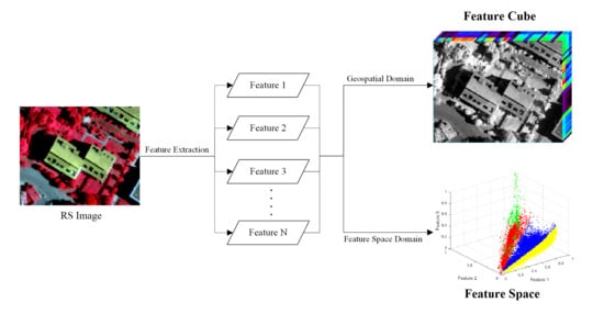
2.1. From the Perspective of the Geospatial Domain

From the perspective of the geospatial domain, RS images are composed of many different ground objects, such as trees, houses, and water bodies. For the objects in an RS image, the spatial distribution of their internal pixels is usually as illustrated in Figure 1 [32]. Specifically, mixed pixels with different mixing levels (e.g., pixels in part C in Figure 1) tend to appear at the boundary of various objects in the image. Moreover, since the pixels that are close to the boundary of the object (e.g., the pixels in Figure 1B) are usually affected by the spectral reflection of the other types of adjacent objects, whose features typically have different degrees of change, thus resulting in a certain difference between the features of these pixels and the features of the object to which these pixels belong. The closer the pixels are to the boundary, the more they are affected and the greater this difference is. Therefore, these mixed pixels and the pixels close to the boundary of the object tend to have significant differences from the surrounding neighborhood pixels. Moreover, they tend to have high classification uncertainty and are easily misclassified in an image classification task because they are mixed with the features of other categories in different proportions. However, the object’s central pixels (e.g., pixels in part A in Figure 1), which are far from object’s boundary, are hardly affected by the spectral reflection of other adjacent objects. Thus, their features tend to be relatively pure and consistent. In other words, they are less different from the surrounding neighborhood pixels. During image classification, these pixels tend to have low uncertainty and are easily classified correctly. For random noises in the image (e.g., the pixels in Figure 1D), their features are random and frequently have significant differences with the surrounding neighborhood pixels. Thus, they have very high uncertainty and are very easily misclassified in image classification. From the abovementioned analysis, we can conclude that the pixels with high uncertainty, such as noises, mixed pixels at the boundary of the object, and pixels close to the boundary of the object, have a common characteristic in that their features are generally different from those of their surrounding neighborhood pixels in the geospatial domain. Conversely, for pixels with low uncertainty, such as central pixels far from the boundary of the object, the difference between their features and the features of their surrounding neighborhood pixels is very small in the geospatial domain. On this basis, we can quantitatively measure and model the uncertainty of the features of different pixels in the geospatial domain.
As shown in Figure 2, from the perspective of the geospatial domain, the n-dimensional features extracted from image X can be constructed into a “feature cube”, which is formed by stacking the n-dimensional features of the image layer by layer. The n-layer features in this cube can be viewed as the description and expression of information from various ground objects in the same geospatial range from n different aspects. Evidently, various feature layers have certain differences in their ability to record and express information of ground objects, so their degree of uncertainty is also different. Thus, the differences between the uncertainties contained in various feature layers must be considered when modeling and measuring the uncertainty of features in the geospatial domain (that is, different features should be treated distinctly).

2.2. From the Perspective of the Feature Space Domain

As shown in Figure 2, from the perspective of the feature space domain, an image X with n-dimensional features can be regarded as a set of feature points in an n-dimensional coordinate system, which is also called a feature space. Every feature point in the n-dimensional coordinate system corresponds to one pixel in the image. In an ideal case, the feature points in the feature space should be densely clustered near several cluster centers (that is, the corresponding feature centers of various categories), and the number of cluster centers is the number of categories in the image. However, in reality, the distribution of feature points in the feature space naturally has different degrees of uncertainty due to many uncertain factors, such as image noises, mixed pixels, and intra-class differences. Figure 3a demonstrates a feature space that corresponds to a real RS image. As shown in Figure 3a, pixels with high uncertainty, such as mixed pixels, are frequently distributed at the boundaries of several clusters, which is why they are easily misclassified during image classification. For pixels with low uncertainty, such as pure pixels, they tend to gather closely near the cluster centers in the feature space. Moreover, during image classification, the lower the uncertainty of the features of the pixels is, the closer the feature points corresponding to these pixels are to the cluster center in the feature space, and vice versa. According to the intensity of the distribution of feature points in the feature space, we can find that the lower the uncertainty of the feature points is, the closer they are to the cluster center, and the higher the density of feature points distributed around them is. Otherwise, the higher the uncertainty of the feature points is, the closer they are to the boundary of the clusters, and the lower the density of feature points distributed around them is. Thus, based on the relationship between the feature uncertainty of the pixels and the intensity of the distribution of feature points around their corresponding feature points in the feature space, the feature uncertainty of the pixels can be quantified and modeled from the perspective of the feature space. That is, the distribution intensity of the feature points is used in the feature space domain. In particular, the denser the distribution of feature points in the feature space is, the lower their uncertainty is. Furthermore, the sparse distribution of feature points denotes their high uncertainty.

3. Approach for Modeling and Measurement of Feature Uncertainty

Feature uncertainty is derived from the confusion of features between different classes of pixels caused by mixed pixels, noises, and the phenomenon where the same objects have different spectra or different objects have the same spectra, which will result in confusion between the categories of these pixels in image classification. In Section 2, we have analyzed the appearance the characteristics of feature uncertainty from the geospatial and feature space domains. Therefore, we can construct the corresponding quantitative models to measure the feature uncertainty of an image according to these characteristics. Correspondingly, in this section, we first measure and model the uncertainty of features from the perspective of geospatial and feature space domains and then combine them to form a feature uncertainty index to describe the uncertainty of image features more accurately and effectively. The specific approach is presented as follows.

3.1. Geospatial Domain

According to the characteristics of feature uncertainty analyzed in Section 2, from the perspective of the geospatial domain, pixels with a high feature uncertainty tend to have significant differences in features from other adjacent neighboring pixels (such as mixed pixels, noises, and the pixels close to the object boundary), whereas pixels with low feature uncertainty tend to have fewer difference in features from other pixels adjacent to them. Thus, the uncertainty of pixel features is high when the difference between features of this pixel and its neighborhood pixels is large, and vice versa. On this basis, we can quantitatively describe and measure the feature uncertainty of pixels in the geospatial domain. In addition, as analyzed in Section 2, various features have certain differences in the ability to record and express ground information. Thus, the difference between the uncertainties contained in the different features must be considered when measuring the uncertainty of image features. To this end, a Local Adaptive Multi-Feature Weighting Method based on Information Entropy is proposed to measure the feature uncertainty of the image in the geospatial domain when we use the multi-dimensional features of the image to describe and model its feature uncertainty comprehensively. The proposed method uses the information entropy in the neighborhood of the target pixel as the weight and calculates the weighted summation of the uncertainties of different features to obtain the comprehensive feature uncertainty of the pixel in the geospatial domain. The specific implementation process is presented as follows.

3.1.1. Uncertainty of the Single-Dimension Feature in the Geospatial Domain

We first calculate the feature uncertainty of the image in each dimension feature. Let P i j be a pixel in image X. In the n-th-dimensional feature of the image, the K*K neighborhood centered on P i j is represented by O p i j n (including the central pixel P i j ) and n = 1 , 2 , , N , where N is the total dimension of the extracted features from image X. Figure 4 depicts an example of the K*K neighborhood O p i j n of pixel P i j (K = 5). Pixel P x y is the pixel of the x-th row and the y-th column in the K*K neighborhood O p i j n . In addition, the n-th-dimensional features of pixel P i j and pixel P x y are represented by f p i j n and f p x y n , respectively.
As mentioned previously, the feature uncertainty of a pixel is high in the geospatial domain when the difference between its features and the features of its surrounding neighborhood pixels is large. Thus, feature uncertainty U p i j n of pixel P i j in the n-th-dimensional feature can be calculated using Equation (1):
U p i j n = p x y O p i j n w p x y · | f p x y n f p i j n | K 2 1 ,
where w p x y represents the weight of the influence of pixel P x y on target pixel P i j , which is determined by the distance from pixel P x y to pixel P i j . According to the first law of geography [33,34], the weight is high when the distance is small, and vice versa. The calculation method of w p x y is expressed in Equation (2):
w p x y = 1 D x y x = 1 K y = 1 K 1 D x y ,
D x y = ( x K + 1 2 ) 2 + ( y K + 1 2 ) 2 + 1 x , y ( 1 , 2 , 3 K ) ,
where x and y correspond to the row and column numbers of pixel P x y in the K*K neighborhood O p i j n of pixel P i j , and D x y represents the distance from pixel P x y to the central pixel P i j . The last "+1" term in Equation (3) is used to prevent the case of D x y = 0 . When the pixel P x y overlaps with the central pixel P i j (that is, x = K + 1 2 and y = K + 1 2 ), D x y = 0 , which is not conducive to the calculation of weights ( w p x y ).

3.1.2. Weights of Different Features

As analyzed in Section 2, various features have certain differences in their ability to record and express ground information, and their degree of uncertainty is also different. Thus, various features must be given different weights when measuring the feature uncertainty of an image.
This study presents a Local Adaptive Multi-Feature Weighting Method based on Information Entropy to describe the feature uncertainty of an image in the geospatial domain. The proposed method uses the information entropy in the local neighborhood of the target pixel as the weight to combine the uncertainty of different features through the weighted summation method. Shannon’s information entropy theory [35] states that the higher the entropy is, the more information contained in the local neighborhood, thereby indicating that the complexity of the neighborhood is higher. Thus, the corresponding weight should be greater. In each dimension feature, the weight and entropy of each pixel is automatically determined on the basis of the difference in the pixels’ features within the local neighborhood of the pixel. That is, the proposed method adaptively determines the weight of each pixel in different feature dimensions. Moreover, the weight of the feature uncertainty of different pixels in the same dimension feature is different, which can more accurately describe the spatial heterogeneity of the feature uncertainty of the image. The calculation method of the weight for every pixel in each dimension feature is described as follows.
According to the information entropy theory [35], in the n-th-dimensional feature, the information entropy of the local K*K neighborhood O p i j n of pixel P i j (that is, the weight of the uncertainty of the nth-dimensional feature of pixel P i j ) is calculated using Equation (4):
E p i j n = p x y O p i j n p p x y log 2 p p x y ,
p p x y = | f p x y n 1 K 2 · p x y O p i j n f p x y n | p x y O p i j n | f p x y n 1 K 2 · p x y O p i j n f p x y n | ,
where pixel P x y is the pixel of the x-th row and the y-th column in the K*K neighborhood O p i j n of pixel P i j in the n-th-dimensional feature.

3.1.3. Integrating Uncertainties of Different Features to Measure the Comprehensive Feature Uncertainty in the Geospatial Domain

Based on the calculated uncertainty of each dimension feature of the pixel and its weight, we use the weighted summation method to combine the uncertainties of different features for obtaining the comprehensive feature uncertainty of every pixel in the geospatial domain. For pixel P i j in image X with n-dimensional features, its comprehensive feature uncertainty in the geospatial domain can be calculated using Equation (6):
U p i j = n = 1 N U p i j n · E p i j n ,
Finally, after normalizing the feature uncertainty of all pixels in the image by using Equation (7), a normalized measurement index of the feature uncertainty of the entire image in the geospatial domain can be obtained and is referred to as GeoSpatial Uncertainty (GSU):
G S U = U min ( U ) max ( U ) min ( U ) ,
where U represents the feature uncertainty of all pixels in the geospatial domain before normalization, U = { U p i j | P i j X } , and max ( U ) and min ( U ) represent the maximum and minimum values of U , correspondingly.

3.2. Feature Space Domain

According to the analysis presented in Section 2, ideally, different categories of pixels in an image will form several very dense cluster centers in the feature space. However, due to the influence of many uncertainty factors, such as inter-class similarities, mixed pixels, and noise, not all feature points are very densely distributed in the feature space. Moreover, the feature points with low feature uncertainty are frequently distributed near the cluster centers, and the lower the uncertainty of the feature points, the greater the distribution density of the feature points around them. By contrast, the feature points with high feature uncertainty tend to be discrete in the feature space, and the higher the uncertainty of the feature points, the smaller the distribution density of the feature points around them.
Thus, we can quantify and model the feature uncertainty of pixels in the feature space domain based on the distribution law of the feature points with different degrees of feature uncertainty in the feature space.
Here, we propose the Local Distribution Density of Points (LDDP) to measure the intensity of the distribution of feature points in the feature space and use it to represent the feature uncertainty of pixels in the feature space domain. In this study, as shown in Figure 3b, the LDDP ( Φ i ) of the i-th feature point P in the feature space (corresponding to the i-th pixel P in the image) is defined as the average of the distances between the m feature points closest to P and point P in the feature space. LDDP is calculated using Equation (8):
Φ i = 1 m j = 1 m d i j ,
where d i j represents the Euclidean distance from the j-th feature point closest to the current feature point P to point P, j = 1, 2, … m; d i j can be calculated using Equation (9) [36]:
d i j = n = 1 N ( f i n f j n ) 2 ,
where f i n and f j n represent the n-th feature of the current i-th pixel P and its j-th nearest pixel in the feature space, correspondingly, n = 1 , 2 , , N , where N is the total dimension of features of the image.
The LDDP of all pixels in the feature space can be obtained by traversing each pixel in the image (that is, each feature point in the feature space). As previously mentioned, the difference in the LDDP between different pixels reflects the variation in feature uncertainty between different pixels in the feature space domain. Thus, we can normalize the LDDPs of all pixels in the entire image by using Equation (10) and use the normalized LDDP to measure the feature uncertainty of the pixels (feature points) in the feature space domain, referred to as the Feature Space Uncertainty (FSU):
F S U = Φ min ( Φ ) max ( Φ ) min ( Φ ) ,
where Φ represents the LDDP of all pixels in the image, and the max ( Φ ) and min ( Φ ) represent the maximum and minimum values of the LDDP of all pixels, respectively.

3.3. Feature Uncertainty Index Integrated Geospatial and Feature Space Domains

GeoSpatial Uncertainty (GSU) and Feature Space Uncertainty (FSU) describe the feature uncertainty of an image from two different domains. Generally, the feature uncertainty of an image can be more effectively and comprehensively described and measured by reasonably integrating the two domains. Thus, this study integrates GSU and FSU to obtain a new Feature Uncertainty Index (FUI) to comprehensively describe and quantify the feature uncertainty of an image. FUI is calculated using Equation (11):
F U I = ( 1 λ ) · G S U + λ · F S U ,
where the non-negative constant λ is the adjustment coefficient and is used to adjust the weights of the geospatial and feature space domains.

4. Validation Schemes

To verify the validity of the proposed feature uncertainty modeling approach (that is, the constructed index FUI), this study improves the verification strategy in the literature [31] and tests the effectiveness of the approach from two aspects: (i) Statistical analysis: Statistical analysis of the correlation between classification error rate and feature uncertainty (which is measured by FUI) in the image classification results. In theory, the higher the feature uncertainty of the pixels, the more likely they are to be misclassified during image classification [14]. Thus, in the classification results, the classification error rate and feature uncertainty should have a significantly positive correlation. In actual statistics and correlation analysis of the experimental results, if a significant positive correlation does exist between the classification error rate and feature uncertainty, then the proposed feature uncertainty modeling approach is indeed effective. Moreover, the stronger this positive correlation is, the more effective the proposed approach is. (ii) Analysis of the effect on image classification: The FUI constructed by the proposed approach is applied to the image classification process to improve the accuracy of the classification results. If the accuracy of the image classification results is indeed improved by using the FUI in the classification process, then the proposed feature uncertainty modeling approach is indeed effective and valuable [14]. The flowcharts of the two verification schemes are exhibited in Figure 5. Next, the two verification schemes are specifically described below.

4.1. Scheme I: Statistical Analysis

As mentioned above, the higher the feature uncertainty of the pixels in an image, the more likely the pixels are to be misclassified. Thus, in the classification map, the classification error rate is higher in pixels with higher feature uncertainty. In the statistical analysis of the classification results, if this positive correlation does exist between the FUI and classification error, then the proposed approach is effective. The stronger this positive correlation is, the more effective the proposed approach is.
To describe this relationship quantitatively, this study uses the Pearson correlation coefficient to measure the correlation between feature uncertainty measured using the FUI and classification error rate quantitatively. The specific process is expressed as follows.
(1) Selecting an appropriate method for image classification:
The statistical analysis in the experiments is based on the image classification results. Thus, it is necessary to select appropriate classification methods to classify the image for subsequent statistical analysis. SVM is a machine learning algorithm based on statistical learning theory. It has evolved into a well-developed and widely used classical classification method in image classification [2,3,37]. Therefore, the SVM classification algorithm is used in this study for image classification.
Notably, to facilitate the verification of the second scheme, an SVM soft classification method is used to classify the image here, and the soft classification results are hardened on the basis of the principle of maximum membership to obtain the final classification results [38]. That is, each pixel is classified into the category that corresponds to its maximum membership. The soft classification results and hardened classification map are used in the second scheme. Moreover, SVM soft classification is implemented by using the open-source LibSVM tool [39]. Additional details on the SVM soft classification can be found in the literature [39,40].
(2) Determining the range of valid values for the FUI:
Some abnormally large or small values are inevitable in the calculated FUI due to the influence of the image noise. In subsequent statistical analyses, a division of the different levels of feature uncertainty and related statistics will be performed. If these abnormal values are not excluded, they will affect the accuracy and reliability of the results of subsequent statistical analyses. Thus, we must determine an effective and reliable range of values for the FUI. In the present study, the range of valid values for the FUI is determined on the basis of its valid maximum and minimum values.
According to the 3δ theory in statistics [41], we determine that the valid maximum and minimum values of FUI are v a l u e max and v a l u e min , respectively, and their expressions are presented in Equation (12):
v a l u e min = μ 3 δ v a l u e max = μ + 3 δ ,
where μ and δ are the mean and standard deviation of the FUI of all pixels in the entire image, correspondingly.
Thus, in the image, only pixels with feature uncertainties in the range [ v a l u e min , v a l u e max ] are included in subsequent statistical analysis. According to statistical theory [41], [ v a l u e min , v a l u e max ] has a confidence interval of 99.74%. In particular, in terms of the FUI, the pixels in [ v a l u e min , v a l u e max ] contain 99.74% of the information of the entire image.
(3) Division of uncertainty levels:
All the pixels in the interval [ v a l u e min , v a l u e max ] are divided into N levels with an equal interval of uncertainty based on the degree of feature uncertainty, and the range of uncertainty that corresponds to the n-th level is expressed as follows:
[ v a l u e min + ( n 1 ) v a l u e max v a l u e min N , v a l u e min + n v a l u e max v a l u e min N ] ,
where n = 1 , 2 , , N , and N represents the total number of the divided uncertainty levels.
(4) Calculation of classification error rates for each feature uncertainty level:
The number of misclassified pixels in each level of uncertainty is first counted from the classification maps. Then, the overall classification error rate δ n of each level is calculated using Equation (14):
δ n = n u m n N U M n ,
where δ n is the overall classification error rate of the n-th level, n u m n is the total number of misclassified pixels within the n-th level, and N U M n is the total number of pixels within the n-th level.
(5) Correlation analysis between classification error rates and feature uncertainty levels:
The correlation coefficient R between the classification error rates and feature uncertainty levels is calculated in accordance with the definition of the Pearson correlation coefficient [42]. The calculation method is expressed as follows:
R = n = 1 N ( δ n δ ¯ ) ( n n ¯ ) n = 1 N ( δ n δ ¯ ) 2 n = 1 N ( n n ¯ ) 2 ,
where δ ¯ and n ¯ represent the average values of δ n and n, respectively; n = 1, 2⋯⋯N; and N is the total number of the divided uncertainty levels.
According to the statistical meaning of Pearson correlation coefficient [42], the larger the absolute value of coefficient R between feature uncertainty levels and classification error rates is, the stronger the correlation between them. Furthermore, they are positively correlated when the coefficient R’s value is positive, and vice versa. Evidently, the stronger the correlation is, the more effective the proposed feature uncertainty modeling approach.

4.2. Scheme II: Analysis of the Effect on Image Classification

In addition to demonstrating the validity of the proposed approach from the perspective of statistical analysis, this study also analyzes the effect of the FUI constructed by using this approach on the reliability and accuracy of the classification results to further confirm the validity and practical value of the proposed approach. Specifically, the calculated FUI is applied to image classification. Theoretically, the reliability of the image classification results can be improved by controlling or constraining the image’s feature uncertainty, which is quantified using the proposed FUI during image classification [14]. Then, the accuracy of the classification results will naturally increase when their reliability is improved. Furthermore, in the experimental results, if the accuracy of classification results is indeed improved by using the proposed FUI, it means that the proposed FUI does play a role, which can prove that the proposed feature uncertainty modeling approach is effective. This verification scheme is subsequently presented in detail.
As stated in the literature [31], the post-processing of image classification is also an important part of the image classification task. Reasonable post-classification methods can effectively improve the preliminary classification maps and enhance the performance and reliability of classification [43,44]. On this basis, the present study applies the FUI calculated by the proposed approach to the post-processing of image classification to improve the accuracy of image classification results.
For the traditional post-processing of image classification, a common method is to refine the initial classification results through spatial filtering (SF) [45], which utilizes the spatial information of an image to maintain the spatial consistency of the image classification map based on the first law of geography [33,34]. For an image soft classification task, after performing SF on each layer from the image initial soft classification results (taking 3 × 3 spatial filtering as an example), the new soft classification results of pixel P (i, j) in the image can be presented by using Equation (16):
ρ P , c = n = 1 9 w n ρ n , c ,
where ρ P , c denotes the probability that pixel P belongs to the c-th category after SF; c = 1 , 2 C ; and C is the total number of categories predefined for image classification. w n and ρ n , c , respectively, represent the weight of the n-th pixel in the eight-neighborhood O p and its probability that it belongs to the c-th category in the initial soft classification results.
For traditional SF, the weight w n of different pixels in the neighborhood of pixel P (i, j) is determined on the basis of its spatial distance to the target pixel P. The weight w n of different pixels can be calculated using Equation (17):
w n = 1 d n n = 1 9 1 d n d n = ( m i ) 2 + ( n j ) 2 + 1 ,
where w n and d n represent the weight of the n-th pixel (m,n) in the neighborhood O p of pixel P and its distance to pixel P, correspondingly. The variables (i, j) and (m, n) represent the map coordinates (row, column) of pixel P and the n-th pixel from the neighborhood O p in the entire image, respectively.
To verify the validity of the proposed approach, we use the calculated FUI to improve the traditional SF method and propose a new Distance and Reliability-based Spatial Filtering (DR_SF) method, which adds uncertainty constraints to the traditional SF to enhance the reliability and accuracy of the filtered results. Specifically, the uncertainty constraint (or reliability) is added to the weight w n of the traditional SF to adjust the weight of the neighboring pixels appropriately. The new adjusted weight is w n , which is calculated using Equation (18).
w n = w n + R n 2 R n = 1 F U I n ,
where F U I n , R n , and w n correspond to the feature uncertainty index, reliability, and new adjusted weight of the n-th pixel in the neighborhood O p . There is an inverse relationship between R n and F U I n and their range of values is [0,1].
The specific implementation process of Scheme II is presented as follows:
(1) We first use the SVM soft classification algorithm to initially classify the RS image, and the results of the preliminary soft classification are obtained. As previously mentioned, the soft classification results from Scheme I are directly used for subsequent verification.
(2) Then, we use the traditional SF and DR_SF to filter and refine each layer of the initial image soft classification results, respectively.
(3) Finally, the new soft classification results are hardened according to the principle of maximum membership [38], and the final classification maps (FCMs) are obtained. Among these FCMs, the FCM obtained through traditional SF is denoted as FCM_SF, and the FCM obtained through DR_SF is recorded as FCM_DR_SF.
Subsequently, the classification accuracies of FCM_SF and FCM_DR_SF are compared and analyzed. If the classification accuracy is higher in FCM_DR_SF than in FCM_SF, it shows that the improved DR_SF filtering method is effective, which further proves the validity of the proposed feature uncertainty modeling approach.

5. Experimental Results and Discussion

5.1. Experimental Data and Settings

To verify the validity and robustness of the proposed feature uncertainty modeling approach, we perform validation experiments on two real RS images (Vaihingen and Potsdam images) by using the two previously designed verification schemes. These images are obtained from the RS image semantic segmentation datasets published by the International Society for Photogrammetry and Remote Sensing (ISPRS) [46]. The ISPRS also provides the corresponding ground truth reference images derived from manual visual interpretation. Obviously, there are some inevitable errors in the determination of the boundary of the object during visual interpretation. Also, pixels with high uncertainty tend to gather near the object boundary. Therefore, to minimize the influence of the ground truths’ errors caused by the inaccurate object boundary on the statistical analysis of the uncertainty (FUI) and final accuracy assessment, the test images used in the experiments are upscaled images (whose spatial resolution is slightly reduced) obtained by pixel aggregation of the original image. Furthermore, the image classification accuracy is evaluated at a sub-pixel scale [31]. The details of the two images and their related experimental parameters are presented as follows.
Vaihingen and Potsdam images are obtained from different airborne image datasets published by the ISPRS for 2D semantic labeling. They consist of three bands (namely, red, green, and blue bands), with a resolution of 9 cm and 5 cm. The original Vaihingen image, Potsdam image, and their corresponding ground truth reference images are illustrated in Figure 6. In actual experiments, the original Vaihingen image is resampled by pixel aggregation from 805 × 620 pixels to 161 × 124 pixels to minimize the influence of the ground truth errors caused by inaccurate visual interpretation on the statistical analysis of the uncertainty (FUI) and final accuracy assessment, and the resampled image has a resolution of 45 cm. The original Potsdam image’s size is 770 × 1500 pixels and is resampled to 154 × 300 pixels during the experiment. The resampled Potsdam image’s resolution is 25 cm. In addition, there are four main categories in the Vaihingen image: impervious surface, buildings, low vegetation, and trees. The Potsdam image mainly includes three types of categories, namely, impervious surfaces, buildings, and low vegetation.
During verification, the image features used in image classification are similar to those used in the modeling and calculation of feature uncertainty (including GSU, FSU, and FUI). These features include spectral and texture features. The spectral features include all the spectral bands of the experimental images. The texture features include features (such as mean, variance, and entropy) extracted from each band of the experimental images by using the Grey Level Co-occurrence Matrix. In addition, the kernel size used to extract texture features is 3 × 3.
In the experiments, three key parameters must be set. These parameters are neighborhood window size K when calculating the GSU, the number m of adjacent feature points when calculating the FSU, and the adjustment coefficient λ , which is used to adjust the weights of the geospatial and feature space domains when calculating the final FUI. In the experiments on the two images, the settings of the three parameters are summarized in Table 1. Evidently, the setting of the three parameters may affect the measurement of feature uncertainty. The discussion of these parameters is presented in detail in the last section.

5.2. Results and Analysis

The GSUs and FSUs of the Vaihingen and Potsdam images are first calculated on the basis of the methods described in Section 3. Then, the GSUs and FSUs are integrated to obtain the final FUIs. The GSUs, FSUs, and FUIs of the two images are depicted in Figure 7.
The images need to be classified before the statistical analysis. The classic SVM algorithm is used in this study. The classification results of the two images are demonstrated in Figure 8a,d.
According to the designed Scheme I, we divide the obtained FUI map into 10 levels with equal uncertainty intervals. Then, in the classification maps exhibited in Figure 8a,d, the classification error rate of each level is calculated, and, finally, scatterplot fitting and a Pearson correlation analysis are performed between the uncertainty levels and classification error rates. The scatterplots and fitted curves are displayed in Figure 9. The correlation coefficients and fitted curve equations are listed in Table 2.
As can be seen from Figure 9 and Table 2, the fitting degree of the curves in the scatterplots is very high, and the levels of uncertainty and classification error rates show a significant positive correlation. That is, the higher the level of uncertainty is, the higher the classification error rate is. Moreover, their positive correlation is very strong. In particular, the correlation coefficient R is greater than 0.98 (Vaihingen: 0.9867 and Potsdam: 0.9818). Thus, from a statistical perspective, the proposed feature uncertainty modeling approach is evidently effective, and its ability to indicate classification errors is very strong.
Based on the Scheme II designed previously, we use SF and DR_SF to refine each layer of the initial image soft classification results and then harden the new soft classification results according to the principle of maximum membership to obtain the final classification maps (FCMs), as illustrated in Figure 8b,c,e,f. As previously mentioned, the FCM obtained through the traditional SF is denoted as FCM_SF, and the FCM obtained through the DR_SF is recorded as FCM_DR_SF. Similarly, the initial soft classification results are also hardened to obtain the original classification map (OCM), as depicted in Figure 8a,d. Finally, we use the Overall Accuracy (OA) and Kappa Coefficient (KC) to evaluate and compare the classification accuracy of the OCM, FCM_SF, and FCM_DR_SF. The results of the accuracy evaluation of OCM, FCM_SF, and FCM_DR_SF are summarized in Table 3.
In Table 3, the accuracies are higher in FCM_SF and FCM_DR_SF than in OCM, regardless of OA or KC, thereby indicating that the accuracy of the classification results is significantly improved after filtering. Moreover, the classification accuracy after filtering is higher through the DR_SF than through the traditional SF (in Table 3, the accuracy is higher in FCM_DR_SF than in FCM_SF), thereby indicating that the improved DR_SF method is effective. Evidently, the only difference between the DR_SF and traditional SF is that DR_SF filtering uses the FUI obtained by the proposed uncertainty modeling approach to constrain or control the feature uncertainty of the images. Now, the improved DR_SF method is confirmed to be effective, thereby indicating that the proposed feature uncertainty modeling approach is indeed effective and valuable and can be used for image classification to improve the accuracy of classification results.

5.3. Discussion of Parameter Sensitivity

The experimental results presented in Section 5.2 confirm the validity of the proposed feature uncertainty modeling approach. To promote the application of the proposed approach in practice, the parameter sensitivity of the approach is discussed as follows.
The proposed approach mainly involves three parameters, namely, the neighborhood window size K when calculating the GSU, the number m of adjacent feature points when calculating the FSU, and the adjustment coefficient λ when calculating the FUI. In the discussion, we use a control variable method [47] to analyze the sensitivity between the three parameters and the measurement accuracy of feature uncertainty in accordance with the designed verification scheme I. Moreover, the correlation coefficient R between the feature uncertainty levels and classification error rates is used to represent the measurement accuracy of feature uncertainty. Specifically, the sensitivity between a parameter and measurement accuracy is analyzed by fixing the value of the two other parameters of the proposed approach. The details of the discussion are presented as follows.
(1) To adjust coefficient λ , we fix the values of K and m (K = 5, m = 15 for Vaihingen; and K = 5, m = 15 for Potsdam) and let the value of λ vary from 0 to 1 at intervals of 0.1. The relationship between parameter λ and the square of correlation coefficient R (R2) for each dataset is depicted in Figure 10.
As shown in Figure 10, the variation of R2 with λ (from small to large) shows a downward trend as a whole, and the downward trend becomes more evident when λ is greater than 0.5. In addition, R2 obtains the maximum value when the value of λ is 0.1–0.2. This condition indicates that the value of λ should not be too large. Especially when λ is greater than 0.5, the measurement accuracy of the proposed uncertainty modeling approach may be significantly reduced. Thus, we recommend that the default value of λ be 0.1–0.2. It should be noted that there are two abnormal points in Figure 10 (0.7 for Vaihingen and 0.9 for Potsdam), which may be caused by abnormal values in the FUI. In Scheme I, we use the 3δ rule [41] to exclude some abnormal values, but there is no guarantee that all abnormal values will be eliminated. Abnormal values may cause inaccuracies in a valid range [ v a l u e min , v a l u e max ] , thereby causing anomalies in R2.
(2) For the neighborhood window size K, we fix the values of λ and m ( λ = 0.2, m = 15 for Vaihingen; and λ = 0.1, m = 15 for Potsdam), and let the value of K vary from 3 to 11 at intervals of 2. The relationship between parameter K and R2 for each dataset is displayed in Table 4.
In Table 4, the change in R2 with K (from small to large) is relatively stable with a small fluctuation, thus indicating that parameter K slightly affects the measurement accuracy of the approach. It should be noted that when the value of K changes, the valid statistical range [ v a l u e min , v a l u e max ] determined by the 3δ rule is not completely the same, which affects the division of uncertainty levels. Therefore, it is acceptable that the R2 obtained by statistical analysis exhibits a nonlinear change with a small fluctuation, while the R2 of the Vaihingen and Potsdam images reaches a maximum at K = 5 and K = 3, respectively, which may be related to the local spatial autocorrelation of the images. According to the first law of geography [33], RS images often show a high correlation in small local neighborhoods. We recommend the default value of K to be approximately 5 for the sake of the accuracy and efficiency of image processing.
(3) For the number m of adjacent feature points, we fix the values of λ and K ( λ = 0.2, K = 5 for Vaihingen; and λ = 0.1, K = 5 for Potsdam) and let the value of m vary from 5 to 25 at intervals of 5. The relationship between parameter m and R2 for each dataset is presented in Table 5.
Table 5 shows that, like the parameter K, the change in R2 with m (from small to large) is also relatively stable overall, thereby indicating that parameter m also slightly influences the measurement accuracy of the proposed approach. Similarly, the nonlinear change with a small fluctuation of R2 may be caused by a change in the valid statistical range [ v a l u e min , v a l u e max ] . We recommend the default value of m to be approximately 10–15 because in a large number of experiments on the two images, R2 can obtain the corresponding maximum value when the values of m are 10 and 15, which may be related to the spatial autocorrelation of images.
Notably, no experiments have been conducted on larger values of K and m because too large a K and m are generally not considered in practical applications.

6. Conclusions

To make up for the lack of research on the quantitative modeling and measurement of the uncertainty of features extracted from RS images, this study proposes a modeling and measurement approach for the uncertainty of image features. Specifically, on the basis of the source and formation mechanism of the feature uncertainty of RS images, the appearance characteristics of feature uncertaintyies are first investigated and summarized in this study from the perspectives of geospatial and feature space domains. The formation of the topic on the classification uncertainty of image features is one of the main innovations of this study. Then, in accordance with these characteristics, a new local adaptive multi-feature weighting method based on information entropy and the local distribution density of points is proposed to quantitatively describe and model the feature uncertainties of images in the geospatial and feature space domains, respectively. Moreover, two uncertainty measurement indices, namely, GeoSpatial Uncertainty (GSU) and Feature Space Uncertainty (FSU) are proposed accordingly in these two domains. After that, the proposed approach effectively integrates GSU and FSU to obtain a new Feature Uncertainty Index (FUI) to comprehensively quantify the feature uncertainty of images. The proposed feature uncertainty modeling approach (include the proposed index FUI) is one of the main contributions of this study.
In addition, to verify the validity of the proposed feature uncertainty modeling approach, two different effectiveness verification schemes are also designed from two perspectives, namely, statistical analysis and image classification. The former analyzes the correlation between the error rates of image classification and the levels of feature uncertainty, which can confirm the validity of the proposed approach and the ability of the calculated FUI to indicate classification errors. The latter proposes an FUI-based uncertainty control method (the DR_SF) to improve the accuracy of image classification results. This improvement can further prove the validity of the proposed approach and its practical value in image classification. In the future, the proposed two verification schemes will also be useful for the validation of uncertainty modeling and quantification results of other stages of image classification, such as the uncertainty quantification of image segmentation.
Finally, the experimental results on two open and real RS images from the ISPRS confirm the validity and practical value of the proposed approach. The ideal parameter setting of the approach is also supported by discussing the sensitivity of the parameters in the approach, which will be beneficial to the practical application of the proposed approach.
The proposed feature uncertainty modeling approach is effective and practical. According to the results of statistical analysis experiments, the FUI calculated by the proposed approach has a favorable indication ability for image classification errors. This ability may contribute to the prediction of the spatial distribution of image classification errors and the spatial evaluation of the accuracy of classification results. The results of the classification verification experiment show that the proposed approach can accurately measure the uncertainty of image features, and the measurement results can be used to control the uncertainty in image classification for improving the reliability and overall accuracy of the classification results. These findings may have guiding significance for research on reliable image classification schemes or uncertainty control methods for image classification.
The main limitation of our proposed approach is that some assumptions on the spatial distribution of pixels in the image object may not be fully satisfied when the spatial resolution of the image is very low (such as MODIS images with a spatial resolution of 250~1000 meters or other images with lower spatial resolution), which could possibly lead to a decline in the validity of the approach. Moreover, the spatial resolution of the images used in the experiments is high, and the applicability of the proposed approach to low-resolution images should be tested and verified further. Therefore, in future research, we will continue to use images with different types of low, medium, and high spatial resolutions to further test and analyze the validity, applicability, and robustness of the proposed approach and optimize it accordingly.
In the future, we will also further investigate and design more effective uncertainty control methods or strategies based on the proposed model to improve the reliability and accuracy of the image classification results. Furthermore, the propagation laws of uncertainty at different stages of image classification, and the mechanisms behind the influence of these laws on the classification results, will also be thoroughly studied.

Author Contributions

Q.Z. and P.Z. were responsible for the overall design of the study. Q.Z. and Y.X. performed all the experiments. Q.Z. drafted the manuscript. P.Z. provided ideas to improve the quality of the paper. All authors read and approved the final manuscript.

Funding

This research was funded by “The National Key Research and Development Program of China” (2018YFF0215006). It was also funded by the Geomatics Technology and Application key Laboratory of Qinghai Province (Grant No.QHDX-2018-09).

Acknowledgments

The authors would like to thank the International Society for Photogrammetry and Remote Sensing (ISPRS) for providing the datasets. The authors are also grateful to the anonymous referees for their constructive criticism and insightful suggestions.

Conflicts of Interest

The authors declare no conflict of interest.

References

  1. Murthy, C.S.; Raju, P.V.; Badrinath, K.V.S. Classification of wheat crop with multi-temporal images: Performance of maximum likelihood and artificial neural networks. Int. J. Remote Sens. 2003, 24, 4871–4890. [Google Scholar] [CrossRef]
  2. Melgani, F.; Bruzzone, L. Classification of hyperspectral remote sensing images with support vector machines. IEEE Trans. Geosci. Remote Sens. 2004, 42, 1778–1790. [Google Scholar] [CrossRef] [Green Version]
  3. Mountrakis, G.; Im, J.; Ogole, C. Support vector machines in remote sensing: A review. ISPRS J. Photogramm. Remote Sens. 2011, 66, 247–259. [Google Scholar] [CrossRef]
  4. Belgiu, M.; Drăguţ, L. Random forest in remote sensing: A review of applications and future directions. ISPRS J. Photogramm. Remote Sens. 2016, 114, 24–31. [Google Scholar] [CrossRef]
  5. Xia, J.; Du, P.; He, X.; Chanussot, J. Hyperspectral Remote Sensing Image Classification Based on Rotation Forest. IEEE Geosci. Remote Sens. 2014, 11, 239–243. [Google Scholar] [CrossRef]
  6. Blaschke, T. Object based image analysis for remote sensing. ISPRS J. Photogramm. Remote Sens. 2010, 65, 2–16. [Google Scholar] [CrossRef] [Green Version]
  7. Zhang, P.; Lv, Z.; Shi, W. Object-Based Spatial Feature for Classification of Very High Resolution Remote Sensing Images. IEEE Geosci. Remote Sens. Lett. 2013, 10, 1572–1576. [Google Scholar] [CrossRef]
  8. Bialas, J.; Oommen, T.; Havens, T.C. Optimal segmentation of high spatial resolution images for the classification of buildings using random forests. Int. J. Appl. Earth Obs. Geoinf. 2019, 82, 101895. [Google Scholar] [CrossRef]
  9. Gonçalves, J.; Pôças, I.; Marcos, B.; Mücher, C.A.; Honrado, J.P. SegOptim—A new R package for optimizing object-based image analyses of high-spatial resolution remotely-sensed data. Int. J. Appl. Earth Obs. Geoinf. 2019, 76, 218–230. [Google Scholar] [CrossRef]
  10. Hossain, M.D.; Chen, D. Segmentation for Object-Based Image Analysis (OBIA): A review of algorithms and challenges from remote sensing perspective. ISPRS J. Photogramm. Remote Sens. 2019, 150, 115–134. [Google Scholar] [CrossRef]
  11. Zhang, L.; Zhang, L.; Du, B. Deep Learning for Remote Sensing Data: A Technical Tutorial on the State of the Art. IEEE Geosci. Remote Sens. Mag. 2016, 4, 22–40. [Google Scholar] [CrossRef]
  12. Zhu, X.X.; Tuia, D.; Mou, L.; Xia, G.; Zhang, L.; Xu, F.; Fraundorfer, F. Deep Learning in Remote Sensing: A Comprehensive Review and List of Resources. IEEE Geosci. Remote Sens. Mag. 2017, 5, 8–36. [Google Scholar] [CrossRef] [Green Version]
  13. Romero, A.; Gatta, C.; Camps-Valls, G. Unsupervised Deep Feature Extraction for Remote Sensing Image Classification. IEEE Trans. Geosci. Remote Sens. 2016, 54, 1349–1362. [Google Scholar] [CrossRef]
  14. Shi, W.Z. Principles of Modelling Uncertainties in Spatial Data and Spatial Analyses; CRC Press: Boca Raton, FL, USA, 2008. [Google Scholar]
  15. Hand, D.J. Measurements and their Uncertainties: A Practical Guide to Modern Error Analysis by Ifan G. Hughes, Thomas P. A. Hase. Int. Stat. Rev. 2011, 79, 280. [Google Scholar] [CrossRef]
  16. Stastny, J.; Skorpil, V.; Fejfar, J. Visualization of uncertainty in LANDSAT classification process. In Proceedings of the 2015 38th International Conference on Telecommunications and Signal Processing (TSP), Prague, Czech Republic, 9–11 July 2015; pp. 789–792. [Google Scholar]
  17. Choi, M.; Lee, H.; Lee, S. Weighted SVM with classification uncertainty for small training samples. In Proceedings of the 2016 IEEE International Conference on Image Processing (ICIP), Taipei, Taiwan, 25–28 September 2016; pp. 4438–4442. [Google Scholar]
  18. Wilson, R.; Granlund, G.H. The Uncertainty Principle in Image Processing. IEEE Trans. Pattern Anal. Mach. Intell. 1984, PAMI-6, 758–767. [Google Scholar] [CrossRef]
  19. Carmel, Y. Controlling data uncertainty via aggregation in remotely sensed data. IEEE Geosci. Remote Sens. Lett. 2004, 1, 39–41. [Google Scholar] [CrossRef]
  20. Li, W.; Zhang, C. A Markov Chain Geostatistical Framework for Land-Cover Classification With Uncertainty Assessment Based on Expert-Interpreted Pixels From Remotely Sensed Imagery. IEEE Trans. Geosci. Remote Sens. 2011, 49, 2983–2992. [Google Scholar] [CrossRef]
  21. Gillmann, C.; Wischgoll, T.; Hagen, H. Uncertainty-Awareness in Open Source Visualization Solutions. In Proceedings of the IEEE Visualization Conference (VIS)—VIP Workshop, Baltimore, MD, USA, 23–28 October 2016. [Google Scholar]
  22. Gillmann, C.; Arbelaez, P.; Hernandez, T.J.; Hagen, H.; Wischgoll, T. An Uncertainty-Aware Visual System for Image Pre-Processing. J. Imaging 2018, 4, 109. [Google Scholar] [CrossRef]
  23. Giacco, F.; Thiel, C.; Pugliese, L.; Scarpetta, S.; Marinaro, M. Uncertainty Analysis for the Classification of Multispectral Satellite Images Using SVMs and SOMs. IEEE Trans. Geosci. Remote Sens. 2010, 48, 3769–3779. [Google Scholar] [CrossRef] [Green Version]
  24. Feizizadeh, B. A Novel Approach of Fuzzy Dempster–Shafer Theory for Spatial Uncertainty Analysis and Accuracy Assessment of Object-Based Image Classification. IEEE Geosci. Remote Sens. 2018, 15, 18–22. [Google Scholar] [CrossRef]
  25. Gillmann, C.; Post, T.; Wischgoll, T.; Hagen, H.; Maciejewski, R. Hierarchical Image Semantics using Probabilistic Path Propagations for Biomedical Research. IEEE Comput. Graph. Appl. 2019. [Google Scholar] [CrossRef]
  26. Shi, W.; Zhang, X.; Hao, M.; Shao, P.; Cai, L.; Lyu, X. Validation of Land Cover Products Using Reliability Evaluation Methods. Remote Sens. 2015, 7, 7846–7864. [Google Scholar] [CrossRef] [Green Version]
  27. Chen, Y.; Jiang, H.; Li, C.; Jia, X.; Ghamisi, P. Deep Feature Extraction and Classification of Hyperspectral Images Based on Convolutional Neural Networks. IEEE Trans. Geosci. Remote Sens. 2016, 54, 6232–6251. [Google Scholar] [CrossRef] [Green Version]
  28. Jia, X.; Kuo, B.; Crawford, M.M. Feature Mining for Hyperspectral Image Classification. Proc. IEEE 2013, 101, 676–697. [Google Scholar] [CrossRef]
  29. Bioucas-Dias, J.M.; Plaza, A.; Camps-Valls, G.; Scheunders, P.; Nasrabadi, N.; Chanussot, J. Hyperspectral Remote Sensing Data Analysis and Future Challenges. IEEE Geosci. Remote Sens. Mag. 2013, 1, 6–36. [Google Scholar] [CrossRef]
  30. Liu, B.; Yu, X.; Zhang, P.; Yu, A.; Fu, Q.; Wei, X. Supervised Deep Feature Extraction for Hyperspectral Image Classification. IEEE Trans. Geosci. Remote Sens. 2018, 56, 1909–1921. [Google Scholar] [CrossRef]
  31. Zhang, Q.; Zhang, P. An Uncertainty Descriptor for Quantitative Measurement of the Uncertainty of Remote Sensing Images. Remote Sens. 2019, 11, 1560. [Google Scholar] [CrossRef]
  32. Cao, S.; Yu, Q.; Zhang, J. Automatic division for pure/mixed pixels based on probabilities entropy and spatial heterogeneity. In Proceedings of the 2012 First International Conference on Agro-Geoinformatics (Agro-Geoinformatics), Shanghai, China, 2–4 August 2012; pp. 1–4. [Google Scholar]
  33. Lv, Z.; Zhang, P.; Atli Benediktsson, J. Automatic Object-Oriented, Spectral-Spatial Feature Extraction Driven by Tobler’s First Law of Geography for Very High Resolution Aerial Imagery Classification. Remote Sens. 2017, 9, 285. [Google Scholar] [CrossRef]
  34. Tobler, W.R. A Computer Movie Simulating Urban Growth in the Detroit Region. Econ. Geogr. 1970, 46, 234–240. [Google Scholar] [CrossRef]
  35. Shannon, C.E. A mathematical theory of communication. Bell Syst. Tech. J. 1948, 27, 379–423. [Google Scholar] [CrossRef]
  36. Li, J.; Lu, B.-L. An adaptive image Euclidean distance. Pattern Recognit. 2009, 42, 349–357. [Google Scholar] [CrossRef]
  37. Cortes, C.; Vapnik, V. Support-vector networks. Mach. Learn. 1995, 20, 273–297. [Google Scholar] [CrossRef]
  38. Kang, X.; Li, S.; Benediktsson, J.A. Spectral–Spatial Hyperspectral Image Classification With Edge-Preserving Filtering. IEEE Trans. Geosci. Remote Sens. 2014, 52, 2666–2677. [Google Scholar] [CrossRef]
  39. Chang, C.-C.; Lin, C.-J. LIBSVM: A library for support vector machines. ACM Trans. Intell. Syst. Technol. 2011, 2, 27. [Google Scholar] [CrossRef]
  40. Wu, T.-F.; Lin, C.-J.; Weng, R.C. Probability Estimates for Multi-class Classification by Pairwise Coupling. J. Mach. Learn. Res. 2004, 5, 975–1005. [Google Scholar]
  41. Pukelsheim, F. The Three Sigma Rule. Am. Stat. 1994, 48, 88–91. [Google Scholar] [CrossRef]
  42. Stigler, S.M. Francis Galton’s Account of the Invention of Correlation. Stat. Sci. 1989, 4, 73–79. [Google Scholar] [CrossRef]
  43. Huang, X.; Lu, Q.; Zhang, L.; Plaza, A. New Postprocessing Methods for Remote Sensing Image Classification: A Systematic Study. IEEE Trans. Geosci. Remote Sens. 2014, 52, 7140–7159. [Google Scholar] [CrossRef]
  44. Cui, G.; Lv, Z.; Li, G.; Atli Benediktsson, J.; Lu, Y. Refining Land Cover Classification Maps Based on Dual-Adaptive Majority Voting Strategy for Very High Resolution Remote Sensing Images. Remote Sens. 2018, 10, 1238. [Google Scholar] [CrossRef]
  45. Lv, Z.; Shi, W.; Benediktsson, A.J.; Ning, X. Novel Object-Based Filter for Improving Land-Cover Classification of Aerial Imagery with Very High Spatial Resolution. Remote Sens. 2016, 8, 1023. [Google Scholar] [CrossRef]
  46. Rottensteiner, F.; Sohn, G.; Jung, J.; Gerke, M.; Baillard, C.; Benitez, S.; Breitkopf, U. The ISPRS benchmark on urban object classification and 3D building reconstruction. ISPRS Ann. Photogramm. Remote Sens. Spat. Inf. Sci. 2012, I-3, 293–298. [Google Scholar] [CrossRef]
  47. Lv, Z.; Liu, T.; Shi, C.; Benediktsson, J.A.; Du, H. Novel Land Cover Change Detection Method Based on k-Means Clustering and Adaptive Majority Voting Using Bitemporal Remote Sensing Images. IEEE Access 2019, 7, 34425–34437. [Google Scholar] [CrossRef]
Figure 1. Spatial distribution of the different types of pixels in the image objects. (The difference in pixel color represents the difference between the features of the pixels.).
Remotesensing 11 01841 g001
Figure 2. N-dimensional “feature cube” and feature space for a remote sensing (RS) image.
Remotesensing 11 01841 g002
Figure 3. Distribution of different types of pixels (feature points) in the feature space. LDDP, Local Distribution Density of Points. (a) a feature space that corresponds to a real RS image; (b) an example for calculating LDDP of pixel P.
Remotesensing 11 01841 g003
Figure 4. K*K neighborhood O p i j n of pixel P i j (K = 5).
Remotesensing 11 01841 g004
Figure 5. Flowcharts of two verification schemes (LayerN represents the probability map that the image is classified into the N-th class in the soft classification results, and “Hardening” represents the hardening process of soft classification results based on the principle of maximum membership). DR_SF, Distance and Reliability-based Spatial Filtering; SF, Spatial Filtering; FCM, Final Classification Map.
Remotesensing 11 01841 g005
Figure 6. Experimental data: (a) false color original Vaihingen image; (b) ground truth reference for Vaihingen image; (c) true color original Potsdam image; and (d) ground truth reference for Potsdam image.
Remotesensing 11 01841 g006
Figure 7. GeoSpatial Uncertainties (GSUs), Feature Space Uncertainties (FSUs), and Feature Uncertainty indices (FUIs) of Vaihingen and Potsdam images: (a) GSU of Vaihingen; (b) FSU of Vaihingen; (c) FUI of Vaihingen; (d) GSU of Potsdam; (e) FSU of Potsdam; and (f) FUI of Potsdam.
Remotesensing 11 01841 g007
Figure 8. Original classification maps (OCMs), FCM_SFs, and FCM_ DR_SFs of Vaihingen and Potsdam images: (a) OCM of Vaihingen; (b) FCM_SF of Vaihingen; (c) FCM_ DR_SF of Vaihingen; (d) OCM of Potsdam; (e) FCM_SF of Potsdam; and (f) FCM_ DR_SF of Potsdam.
Remotesensing 11 01841 g008
Figure 9. Scatterplots and fitted curves of the levels of uncertainty and classification error rates: (a) Vaihingen and (b) Potsdam images. (x-axis: levels of uncertainty, y-axis: classification error rates).
Remotesensing 11 01841 g009
Figure 10. Relationship between parameter λ and the square of correlation coefficient (R2).
Remotesensing 11 01841 g010
Table 1. Experimental parameter settings.
Data SetKmλ
Vaihingen5150.2
Potsdam3150.1
Table 2. Fitted curve equations and correlation coefficients.
Datasets.Equations of the Fitted CurvesCorrelation Coefficient RR2
Vaihingeny = 0.0348x + 0.05780.98670.9735
Potsdamy = 0.0297x − 0.03650.98180.9640
Table 3. Accuracy evaluation results: OCM represents the original classification map. FCM_SF and FCM_ DR_SF correspond to the final classification maps (FCMs) obtained by using SF and DR_SF. OA, overall accuracy; KC, Kappa coefficient.
Classification mapsOAKC
VaihingenPotsdamVaihingenPotsdam
OCM79.0422%93.0883%0.71440.8883
FCM_SF80.5993%93.7199%0.73520.9014
FCM_ DR_SF80.8998%93.9886%0.73920.9024
Table 4. Relationship between parameter K and the square of correlation coefficient (R2).
K357911
R2Vaihingen0.84730.97350.94180.93530.9466
Potsdam0.9640.95130.92010.92950.9235
Table 5. Relationship between parameter m and the square of correlation coefficient (R2).
m510152025
R2Vaihingen0.97730.99090.97350.97730.9665
Potsdam0.93960.94980.95130.94930.943

