Article

An Effectiveness Evaluation Model for Satellite Observation and Data-Downlink Scheduling Considering Weather Uncertainties

School of Reliability and Systems Engineering, Beihang University, Beijing 100191, China
*
Author to whom correspondence should be addressed.
Remote Sens. 2019, 11(13), 1621; https://doi.org/10.3390/rs11131621
Submission received: 11 June 2019 / Accepted: 2 July 2019 / Published: 8 July 2019

Abstract

:
Low Earth orbit (LEO) satellites play an important role in human space activities, and market demands for commercial uses of LEO satellites have been increasing rapidly in recent years. LEO satellites mainly consist of Earth observation satellites (EOSs), the major commercial applications of which are various sorts of Earth observations, such as map making, crop growth assessment, and disaster surveillance. However, the success rates of observation tasks are influenced considerably by uncertainties in local weather conditions, inadequate sunlight, observation dip angle, and other practical factors. The available time windows (ATWs) suitable for observing given types of targets and for transmitting data back to ground receiver stations are relatively narrow. In order to utilize limited satellite resources efficiently and maximize their commercial benefits, it is necessary to evaluate the overall effectiveness of satellites and planned tasks considering various factors. In this paper, we propose a method for determining the ATWs considering the influence of sunlight angle, elevation angle, and the type of sensor equipped on the satellite. After that, we develop a satellite effectiveness evaluation (SEE) model for satellite observation and data-downlink scheduling (SODS) based on the Availability–Capacity–Profitability (ACP) framework, which is designed to evaluate the overall performance of satellites from the perspective of time resource utilization, the success rate of tasks, and profit return. The effects of weather uncertainties on the tasks’ success are considered in the SEE model, and the model can be applied to support the decision-makers on optimizing and improving task arrangements for EOSs. Finally, a case study is presented to demonstrate the effectiveness of the proposed method and verify the ACP-based SEE model. The obtained ATWs by the proposed method are compared with those by the Systems Tool Kit (STK), and the correctness of the method is thus validated.

1. Introduction

Earth observation satellites (EOSs) use Earth-observing sensors to detect the Earth’s surface and lower atmosphere to obtain information [1]. By using many kinds of remote sensing systems, such satellites can measure a wide range of spatial, spectral, and temporal parameters [2]. Consequently, Earth observation satellites have been recognized as valuable tools for viewing, analyzing, characterizing, and making decisions about our environment. Spectral measurements from satellite remote sensors have been applied in many fields, including national defense construction, economic development, national security, environmental protection, disaster assessment, and land resource surveys [3,4]. According to the satellite database of the Union of Concerned Scientists [5], as of 30 November 2018, a total of 1957 active satellites were orbiting the Earth, 65% of which were owned by three nations, i.e., the United States (849), Russia (152), and China (284). The total number of satellites has been growing sharply in recent years; in 6.5 years from 2012 to 2019, the number increased from 1000 to nearly 2000, while in the previous 6.5 years (from 2005 to 2012) the number had only increased from 800 to 1000 [6]. Among the satellites active on 30 November 2018, 1232 of them (63%) were low Earth orbit (LEO) satellites, i.e., those orbiting at an altitude of less than 2000 km above the Earth’s surface. Since LEO satellites have the property of low propagation delay, they are very suitable for use in multimedia technology, as they should be able to deliver a large amount of information such as image and video signals at a higher data rate, as well as audio signals at a relatively low data rate [7,8].
LEO satellites can execute observation tasks only when passing above the target area, and their success rates are often influenced by local weather conditions, illumination conditions (sunlight angles), seasonal factors, etc. A large amount of image/video data is produced after observation and should be transmitted to ground receiver stations when the satellite passes over them. Therefore, LEO satellites can only execute tasks at certain times [9], which are defined as available time windows (ATWs) in this paper. Only after the acquired data has been transmitted to a ground receiver station can an observation task be considered as completely successful. Some observations can only be made when the footprint of the satellite is illuminated by sunlight [10]. Additionally, the quality of satellite observation missions may also be affected by weather conditions. Moreover, observation missions may fail even within the observable time windows, since the quality of the images may not meet the requirements of accuracy and clarity. Therefore, satellite resources are very limited and are much more costly than terrestrial observation resources (i.e., satellites are power- and bandwidth-constrained) [11]. When observing dynamic targets and regional targets, multiple satellites may be used to conduct joint observation missions, which present more complex multi-type task scheduling problems [1,12,13,14,15]. Thus, developing an effectiveness evaluation method for task scheduling for LEO satellites is important to allow decision-makers to evaluate the effectiveness of planned observation tasks. Increasing the effectiveness of observation tasks increases the number of acquisitions that can be made, and therefore ultimately benefits multitemporal analysis. In fact, in this field, the availability of a substantial number of acquisitions is a determinant of the success of observation missions. Therefore, from this perspective, the availability of images can be considered as a key factor of the quality of satellite observations.
System effectiveness is defined as the ability of a system to meet given quantitative characteristics and service requirements under specified conditions. Effectiveness evaluation involves estimating the overall availabilities, efficiencies, success rates, and commercial returns of a system based on their comprehensive performances in order to support the optimization and improvement of task planning [16]. Effectiveness evaluation models have been studied in a wide variety of applications for many years. Many researchers examined the effectiveness of systems by using various methods, including simulations, analytical calculations, computational workflows, and various factors-based and model-assisted approaches, with the goal of validating the systems’ economic advantages in practice. Kabban et al. (2018) proposed a simulation model by using a time- and cost-efficient method to determine sensitive factors of a structural health monitoring (SHM) system in order to enable SHM validation [17]. Madni et al. (2019) proposed a methodological framework for analyzing investments in and potential gains from satellites, considering system complexity, environmental complexity and regulatory constraints, and system lifespan [18]. Liu et al. (2019) used computational workflows for evaluations of the design of complex system solutions, which were also able to support co-simulations as part of larger workflows including additional auxiliary computational tasks [19]. The Availability–Dependability–Capability (ADC) model, Data Envelopment Analysis (DEA), Analytic Hierarchy Process (AHP), Bayesian network, fuzzy evaluation, etc., are all applicable to effectiveness evaluation. The ADC model is based on the availability model of the Weapons System Effectiveness Industry Advisory Committee (WSEIAC), which is improved and applied in this paper. In the model, system effectiveness is defined as the performance metrics of a system that satisfy the specific requirement of varied missions, and it is a function of availability, dependability, and capability [20]. Xiao et al. (2015) first defined the efficiency of family farms, then used Farrell’s production efficiency measurements to investigate the premise assumptions and the realization condition, and then constructed a model to evaluate the effectiveness of family farms based on a nonparametric DEA method [21]. Wu et al. (2016) adopted AHP to determine the weight of all the evaluation indexes and established an assessment model for campus emergency management capability using the fuzzy comprehensive evaluation method [22]. Kabir et al. (2018) developed a Bayesian belief network (BBN) model to evaluate the performance of an employee considering the dependencies and correlations between performance criteria which is also capable of assessing the credibility of multiple experts and ranking employees for different purposes such as reward, improvement, training, promotion, termination, and compensation [23].
Studies of satellite effectiveness evaluation (SEE) in the literature are relatively limited. Li et al. (2018) focused on the assessment of the coverage effectiveness of remote sensing satellites and proposed a multi-index evaluation method based on index weight using an entropy weight method and AHP [24]. In the mentioned papers [17,18,19,20,21,22,23,24], commercial profit is not within the index system, which means the authors cannot measure the economic value of the task scheduling for satellites. Additionally, the effects of weather uncertainties on different observation targets were not considered. In the present study, we firstly describe the motion of a LEO satellite in an Earth-centered inertial (ECI) coordinate frame and then provide a method for generating the ATWs considering sunlight angles, elevation angles, and sensor types. Systems Tool Kit (STK, formerly Satellite Tool Kit) is a mature software tool that can achieve this functionality, however the product is subject to the International Traffic in Arms Regulations (ITAR), administered by the U.S. Department of State, and the Export Administration Regulations (EAR), administered by the U.S. Department of Commerce [25], which means that STK cannot be used in some cases. We propose this method and attempt to provide an alternative reference for others who engage in relevant research. Secondly, we develop an effectiveness evaluation model for satellite observation and data-downlink scheduling (SODS) based on the Availability–Capacity–Profitability (ACP) framework from the perspectives of satellites’ time availability, the success rates of the planned tasks, and the return rate of task profits, which is a comprehensive model to estimate the overall performance of the satellite task system. Furthermore, we consider the effects of weather uncertainties in the SEE model such that different observation tasks are allowed to have different success rates under different weather conditions. Thirdly, we a case study is provided to verify the proposed models and the result is analyzed.
The rest of this paper is organized as follows: In 
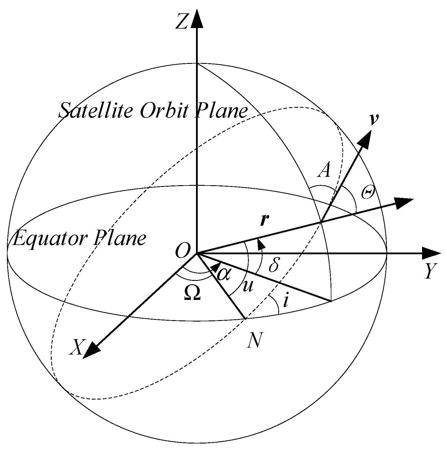
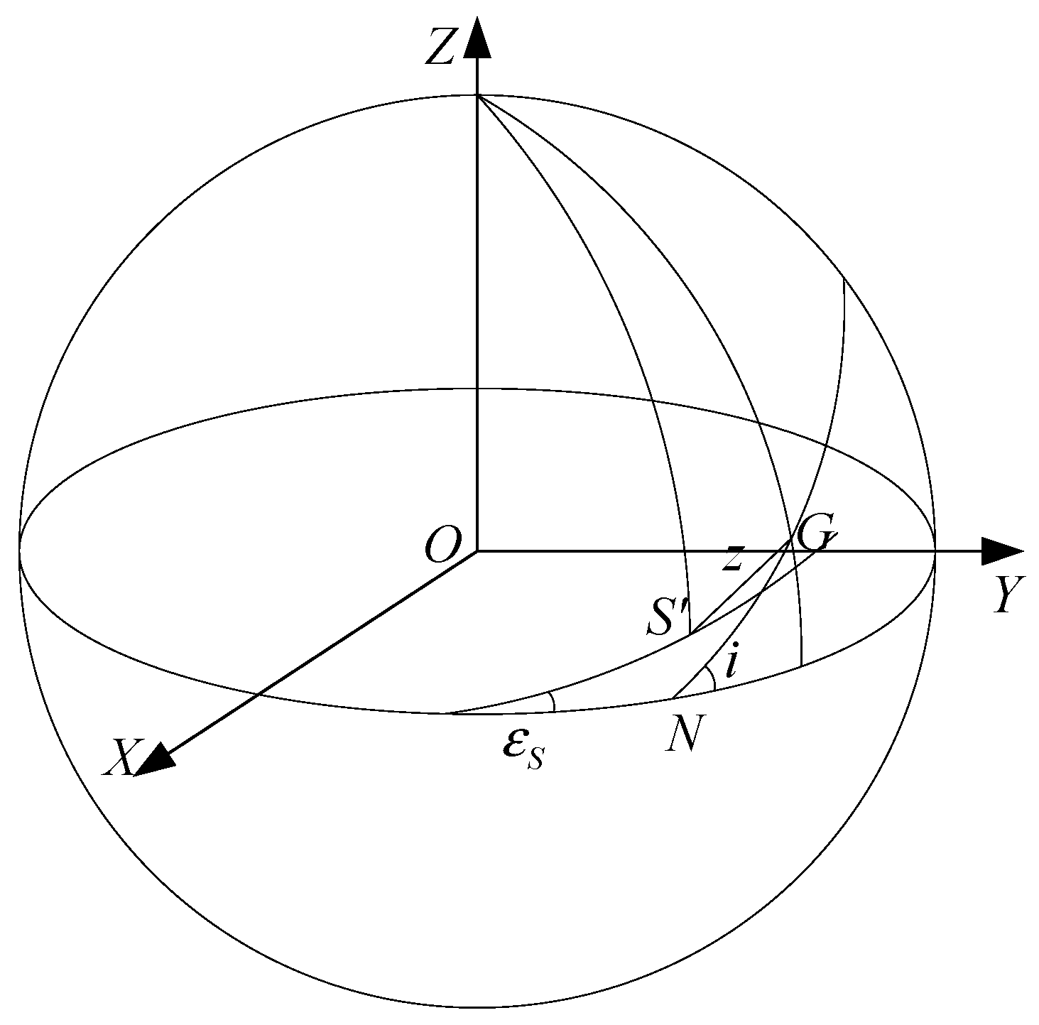
Section 2, we briefly illustrate the two-body motion model and propose a procedure for obtaining ATWs considering some necessary constraints. In Section 3, a formal description of the SEE model for SODS considering weather uncertainties is provided. In this model, the time availability, success rate of observation, rate of return, and mission effectiveness are determined. In Section 4, a case study is presented to demonstrate the effectiveness of the method for obtaining ATWs and the ACP-based SEE model. Finally, in Section 5, we conclude the paper.

2. Method for Obtaining Available Time Windows (ATWs)

2.1. Description of Satellite Orbit

The orbit of a near-Earth satellite is mainly affected by the Earth’s gravitational attraction; however, it is also affected by the gravity of other celestial bodies (such as the sun and the moon). Additionally, the orbits of all satellites are inevitably affected by irregularities in the Earth’s gravitational field as well as density variations in the upper atmosphere, which have been proven to be linked with solar activity and other properties of the atmosphere such as temperature and wind [26]. However, the effects of these perturbations are quite small, and are normally ignored in satellite orbit computations. Here, we consider a two-body motion model involving only the Earth, whose mass is denoted by m1, and a satellite with mass m2, as shown in the inertial coordinate system in Figure 1, where the former is spherically symmetrical and has no atmospheric effect on the satellite and the gravitational attraction is estimated by assuming a point mass at the center of the Earth. The position vector of the center-of-mass C is determined by r C = r 1 m 2 m 1 + m 2 r , where r = r 1 r 2 .
According to Newton’s law of gravitation, the attraction per unit mass at a distance r from the center of a body is GM/r2, where G is the universal constant of gravitation. Thus, the equation of motion of a two-body system is:
r ¨ + μ r 3 r = 0 ,
where r ¨ is the second derivative of the position vector r and μ   =   G ( m 1 + m 2 ) .
The motion of a LEO satellite is described in the spherical coordinate system, as shown in Figure 2, where the coordinate origin is the geocenter, the X-axis direction is the epoch mean vernal equinox, and the Z-axis direction is the epoch mean celestial north pole. Then, an ECI coordinate system is built. The notation and the meaning of the parameters in Figure 2 are illustrated in Table A1 in Appendix A.
Equation (1) is a sixth-order nonlinear system of ordinary differential equations. In order to solve the system completely, we must find the solution that contains six independent integral constants, which should be consistent with the initial value of the motion. Generally, for an elliptical orbit, the orbital elements are σ = ( a , e , i , Ω , ω , τ ) , where a is the major axis of an ellipse, e is the eccentricity, i is the inclination, Ω is the right ascension of the ascending node, ω is the argument of perigee, and τ is the time past perigee. Thus, the polar equation of the ellipse takes the following well-known form:
r = a ( 1 e 2 ) 1 + e cos f ,
where f is the true anomaly, as shown in Figure 3. The satellite passes the perigee when f = 0 and passes the apogee when f = 180°. Particularly, we let
u = ω + f .
Assume that at time t the satellite is at point S, so we have
E e sin E = μ a 3 ( t τ ) .
Thus, the orbital period T of the satellite is obtained by dividing the circumference of the auxiliary circle in Figure 3 by the satellite velocity, which results in
T = 2 π a 3 μ .
Then, the relationship between f and E is
tan f 2 = 1 + e 1 e tan E 2 .
Thus, the declination and right ascension angles can be determined from the formulas for the right spherical triangle, and so we have
δ = arcsin ( sin i sin u )
α = arctan ( cos i tan u ) + Ω .
Since the Earth itself rotates, we use the geocentric longitude λ and geocentric latitude φ to describe the footprint of the satellite. Thus, φ = δ , λ = α S ¯ ( t ) , and S ¯ ( t ) is in Greenwich Mean Time (GMT). For convenience of discussion, we take the time past the ascending node N as the zero time. Then, we have S ¯ ( t ) = S ¯ ( 0 ) + ω E t , and λ and φ can be estimated by the following equations:
φ = arcsin ( sin i sin u )
λ = arctan ( cos i tan u ) + Ω S ¯ ( 0 ) ω E t .

2.2. Function of Calculating ATWs with Multiple Constraints

Figure 4 shows the ground coverage of the satellite. The tangent line between the satellite and the Earth’s surface forms a surrounding ground area, which is the largest ground area that the satellite can observe. However, in the edge of the area, observations may not be suitable to execute due to the obstacle of ground objects. Therefore, we usually need to identify the effective coverage area for observations, which can be determined by the angle σ subtended by the line of SP and the horizon, which is referred to as the minimum viewing angle. The corresponding coverage angle d σ is estimated by Equation (11) as follows:
d σ = arccos ( R e cos σ R e + h ) σ ,
where R e is the radius of the Earth and h = r R e .
Satellite measuring equipment usually has a fixed observation range, which is called the field of view (FOV). We take the conical type of FOV as an example. Let β F O V = F O V / 2 , then d F O V is formulated by
d F O V = arcsin ( sin β F O V R e + h R e ) β F O V .
The coverage angle is
d = min { d σ , d F O V } .
For a low- and medium-orbit Earth satellite, when the coverage angle d is small, the solar illumination requirements for observing ground targets can be approximately regarded as the requirements for the sunlight illumination around the sub-satellite point on the Earth’s surface, as some targets can only be observed in the daytime when the footprint of the satellite is illuminated by sunlight.
Figure 5 shows the sub-solar point. The obliquity of the ecliptic ε S = 23 ° 26 21 . 488 46 . 8150 t 0 . 00059 t 2 , and λ S is the celestial longitude. We use z to represent the zenith distance between the sub-solar point and the sub-satellite point and assume that z 75 ° (i.e., z max = 75 ). Thus, the location vectors of the sun and satellite in the ECI coordinate system are formulated respectively in Equations (14) and (15) as follows:
r S = R 1 ( ε S ) [ cos λ S sin λ S 0 ] ,
r G = R 3 ( Ω ) R 1 ( i ^ ) [ cos u sin u 0 ] ,
where R1 and R2 are rotation matrices and R 1 ( ) = [ 1 0 0 0 cos ( ) sin ( ) 0 sin ( ) cos ( ) ] , R 3 ( ) = [ cos ( ) sin ( ) 0 sin ( ) cos ( ) 0 0 0 1 ] .
Then, we have
cos z = r G r S = A sin u + B cos u ,
where A = sin i sin ε S sin λ S cos i cos Ω cos λ S + cos i cos Ω cos ε S sin λ S and B = cos Ω cos λ S + sin Ω sin λ S cos ε S . Furthermore, let sin ψ = B A 2 + B 2 and cos ψ = A A 2 + B 2 , then we have:
tan ψ = B A   and
β + ψ u 180 β + ψ ,
where sin β = cos z max A 2 + B 2 .
Then, according to Equations (3), (4), and (6), we can determine the time window, denoted as ( t 1 , t 2 ) , that satisfies the light conditions.
Let ( λ 0 , φ 0 ) represent the geocentric longitude and latitude of target A, and let A ( λ 0 , 0 ) represent the projection point of A on the equator plane. As shown in Figure 6, AT0 is then the distance between A and the satellite’s ground track. Since the satellite camera has a valid FOV, there will always be a corresponding covering belt at an angle d to the ground track. Therefore, the target point A can only be observed when the satellite is tracing between T1 and T2. Let t1 and t2 be the times when the satellite passes T1 and T2, respectively, then (t1, t2) is the ATW for observing target A.
Let φ B be the geocentric latitude of point B, then in Δ N A B we have
sin B = cos i cos φ B .
In Δ A B T 0 , we have
sin ( A T 0 ) = sin ( φ 0 φ B ) sin B ,
cos B A T 0 = tan ( A T 0 ) cot ( φ 0 φ B ) ,   and
P A T 0 = π B A T 0 .
In Δ P A T 0 , we have
cos ( P T 0 ) = cos ( 9 0 o φ 0 ) cos ( A T 0 ) + sin ( 9 0 o φ 0 ) sin ( A T 0 ) cos P A T 0 .
The geocentric latitude of point T 0 is φ T 0 = 90 ° P T 0 .
In Δ A T 1 T 0 , we have s = d a E ,
cos T 0 A T 1 = tan ( A T 0 ) tan ( A T 1 ) ,   and
P A T 1 = π B A T 0 + T 1 A T 0 .
In Δ P A T 1 , we have
cos ( P T 1 ) = cos ( 90 ° φ 0 ) cos ( A T 1 ) + sin ( 90 ° φ 0 ) sin ( A T 1 ) cos P A T 1 .
The geocentric latitude of point T1 is φ 1 = 90 ° P T 1 , and we can determine the time t1. In the same way, the time t2 can be determined.
Thus, with the above methods, we can determine the ATWs for observation (ATWOs) for a LEO satellite with elliptical orbits to observe given targets on the Earth’s surface, and also determine the ATWs for transmission (ATWTs) for transmitting the acquired pictures/video to ground station receivers. Multiple constraints are considered in the method which offer some potential benefits, including availability, feasibility, and scalability. Only Equation (4) is a transcendental equation and can be efficiently solved by Newton’s iteration method. The correctness of the method will be validated in Section 4 by comparing the results with STK. The detailed procedure is shown in Appendix A.

3. Satellite Effectiveness Evaluation Model

3.1. Description of Problem

The problem of the SEE of SODS is described as follows: A satellite is assigned with a set of N observation tasks (including data downlink) sequenced in S and Q, where S is the planned observation sequence and Q is the data downlink sequence. Each task j, where jN, is associated with a location with a longitude and latitude, a length of time lj, needed for observing, a length of time τj, needed for data downlink, a set of weather conditions suitable for the observation, a profit revenue, a due time, and a penalty weight for tardiness. The tasks can only be observed in their respective ATWOs, and the produced data can only be transmitted to the ground receiver stations within their respective ATWTs. We assume that the probabilities of weather conditions in ATWOs are known, which can be obtained by weather forecast with much accuracy. Our goal is to evaluate the effectiveness of the satellite using the ACP framework formulated as E = A C P , where A is the time availability indicating the extent to which the satellite’s orbits are available to the given SODS, C is the vector of the success rates of tasks indicating the overall success rate of the SODS affected by weather uncertainties, and P is the vector of the profitability of tasks indicating the net financial gain rates (including tardiness penalties) of the SODS.

3.2. Availability–Capacity–Profitability (ACP)-Based SEE Model Considering Weather Uncertainties

In the following, we propose an ACP-based SEE model to evaluate the effectiveness of a given SODS. The notations used to describe the model are as follows:
Notation list
NSet of observation tasks, n = Card(N)
jIndex of observation tasks, jN
ζTime span of the planning period
MSet of weather types
mIndex of weather types, mM
δjmSuccess rate when observing task j under weather type m
WjSet of ATWOs for task j, T = Card(Wj)
tIndex of time windows in Wj, tWj
(sjt, ejt)Start and end time of the tth ATWO in Wj
wjtmProbability of the tth ATWO of task j having weather type m
W′Set of ATWTs, T’ = Card(W’)
t′Index of time windows in W’, t W
(st, et)Start and end time of the tth ATWTs in W’
ljLength of time needed for observing task j
τjLength of time needed for transmitting data of task j
rjBenefit of task j when completed before the due time
djDue time of task j
fjPenalty weight for the delay of task j
SSequence of tasks for observation
QSequence of tasks for data transmission
zjtBinary parameter representing whether task j is observed in the tth ATWO ( z j t = 1 ) or not ( z j t = 0 )
(xjt, yjt)Scheduled time window to observe task j in the tth ATWO
z′jtBinary parameter representing whether task j is transmitted in the tth ATWT ( z j t = 1 ) or not ( z j t = 0 )
(xjt, yjt)Scheduled time window to transmit data of task j in the t′th ATWT
CjtSuccess rate of observing task j in the tth ATWO
CjOverall success rate of observing task j
FjCompletion time of task j
LjDelay time of task j
PjProfitability of task j
Step 1. Check whether the sequences of observation and transmission fulfill the following conditions or not:
  • The time window scheduled for task j must be within the ATWOs/ATWTs
    { s j t x j t y j t e j t j N , t W j s t x j t y j t e t j N , t W
  • The total observing/transmitting time should be sufficient for task j
    { t W j ( y j t x j t ) l j j N t W ( y j t x j t ) τ j j N
  • The data transmission should start after the observation is finished
    y j t x j t   j N , t W j , t W
Step 2. Calculate the time availability A:
η is the elapsed time during the planning period and μ is length of time that is suitable for observations. The method for calculating η and μ is explained in Algorithm 1. The time availability A reflects the degree of matching of satellite orbit and observation tasks:
A = η μ × 100 % .
Step 3. Calculate the capacity C: the success rates of observations:
A task can be observed in several sequential ATWOs. We assume that the probability of various weather conditions occurring is known, which can be obtained by weather forecast with much accuracy. Success rates when the observing task under each weather type are also known, which can be estimated by the quality of historical observation data. According to this hypothesis, the success rate of the observation of one task is identified:
C j t = { m M δ j m w j t m z j t > 0 1 z j t 0 t W j , j N
C j = t W j C j t
C = [ C 1 , C 2 , C 3 , ] .
Step 4. Calculate the profitability P: gain rates of tasks:
Only after the data acquired by observation has been transmitted to ground receiver stations the task can be considered completely successful. Therefore, the completion time Fj of task j is defined by Equation (34). The task will bring in revenue, however, will also result in a tardiness penalty if it is completed later than the due time. The tardiness penalty is jointly determined by the delay time and penalty weight:
F j = min { τ | τ z j t y j t t W }
L j = max { F j d j , 0 }
P j = r j f j L j r j
P = [ P 1 , P 2 , P 3 , ] T .
Step 5. Definition of the overall effectiveness E:
E = A C P n × 100 % .
The pseudo-code procedure for the above calculations is described in Algorithm 1 as follows.
Algorithm 1 The Availability–Capacity–Profitability (ACP)-based satellite effectiveness evaluation (SEE) model
Input: S, Q, W, W’, M and δ, w, l, τ, r, d, f, z
Output: A, C, P, E
 1: for all j = 1 to n
 2:   for all t = 1 to T, step by 1       /* if the actual time window is within an ATWO and the total length is sufficient*/
 3:    if ( s j t x j t y j t e j t and t W j ( y j t x j t ) l j )
 4:     set the status of the tth ATWO to true
 5:    else
 6:     set the status of the tth ATWO to false
 7:    end if
 8:   end for
 9:   for all t’ = 1 to T’          /* if the actual time window is within an ATWO and the total length is sufficient*/
 10:    if ( s t x j t y j t e t and t W ( y j t x j t ) τ j )
 11:     set the status of the t’th ATWT to true
 12:    else
 13:     set the status of the t’th ATWT to false
 14:    end if
 15:   end for
 16:   if ( j N , t W j , t W , y j t x j t )  /* if the data downlink starts after the observation is finished */
 17:    set the status of S and Q to true
 18:   else
 19:    set the status of S and Q to false
 20:   end if
 21: end for
 22: if all of the status mentioned above is true
 23:   do:
 24:   let η ← 0                /* calculate time availability A */
 25:   for t = 1 to ζ
 26:    if ( j N , t W j , x j t t y j t )
 27:      ηη + 1
 28:    end if
 29:   end for
 30:   let μ ← 0
 31:   for t = 1 to ζ
 32:    if ( j N , t W j , s j t t e j t )
 33:      μμ+1
 34:    end if
 35:   end for
 36:   let A η μ × 100 %
 37:   for all j = 1 to n          /* calculate success rate of observation C */
 38:     for all t = 1 to T
 39:      for all m = 1 to Card(M)
 40:       if ( z j t > 0 )
 41:        let C j t C j t + δ j m w j t m
 42:       else if ( z j t 0 )
 43:        let C j t 1
 44:       end if
 45:     end for
 46:     let C j C j C j t
 47:    end for
 48:  end for
 49:  let C [ C 1 , C 2 , C 3 , ]
 50:  for all j = 1 to n          /* calculate rate of return P */
 51:    for all t’ = 1 to T’
 52:     let F j min { τ | τ z j t y j t t W }
 53:    end for
 54:    let L j max { F j d j , 0 }
 55:    let P j r j f j L j r j
 56:  end for
 57:  let P [ P 1 , P 2 , P 3 , ] T
 58:  let E A C P n × 100 %       /*calculate efficiency E */
 59: end if

4. Case Study of a Low Earth Orbit (LEO) Satellite with Elliptical Orbit

A case study was conducted to illustrate the ACP-based SEE model. The planning horizon is 10 × T , where T is the orbital period of the satellite. Two weather types are considered in ATWOs and each task is assumed to be observed in these two types of weather conditions. Based on a weather forecast, the probabilities of weather types 1 and 2 were set as 90% and 10%, respectively.

4.1. Simulated Satellite Parameters and Model Verification

We suppose that the Earth is a sphere of uniform mass. Parameters of the Earth, the Sun, and satellite are shown in Table 1, Table 2 and Table 3, respectively. The semi-major axis of the elliptical orbit a = 7,378,137 m, and the orbital period T = 2 π a 3 μ E = 6307   s . Figure 7, which was produced by using STK, characterizes orbits of the LEO satellite described above, and five observation targets and three ground receivers are also marked. The benefit rj, due time dj, penalty weight fj, and time length l j / τ j were randomly generated and are shown in Table 4. The satellite’s ATWOs and ATWTs were generated by the algorithm described in Algorithm A1 and calculated by STK are listed in Table 5. STK was used to verify the effectiveness of the proposed method for obtaining ATWs.

4.2. Effectiveness Evaluation and Results Analysis

The sequences of observation and data-downlink are listed in Table 6. In Figure 8, an example is provided to illustrate the internal relations between ATWOs, observation time windows (OTWs), ATWTs, and transmission time windows (TTWs), where the observations of tasks 1–5 are scheduled in OTWs within their own ATWOs, and the data transmissions are scheduled in TTWs within the satellite’s ATWTs.
The result of the evaluation is shown in Table 7. The first step is to check the feasibility of the time window scheduling according to the rules that the satellite can observe only one target at a time, the observations of a task must be scheduled within its ATWOs, the data downlink must be scheduled within the satellite’s ATWTs, and the data downlink of a task must be started after the observation mission is completed. Observation and data transmission for different tasks are allowed to take place at the same time. The steps followed were to calculate A, C, P, and E. The time availability, denoted by A, reflects the extent to which the time resources of the satellite are utilized based on the given observation tasks. It can be used to support the evaluation and optimization of the mission allocation between multiple satellites. The observation success rate C is the expected completion rate of the missions, which can be used to support evaluation and optimization task scheduling. The profitability vector P represents the ratio of the actual commercial benefits of the observation task (including the tardiness penalties) to the expected commercial benefits. E is the overall effectiveness of the satellite.

5. Conclusions and Future Research Directions

Satellite resources are very limited, and their utilization is affected by available time windows, weather conditions, sunlight illumination, and many other factors. For commercial satellites, it is important to make full use of rare satellite resources and to maintain high success rates of observations in order to maximize the net profits when serving market customers. In this paper, a procedure for obtaining available time windows with multiple constraints is presented, and an Availability–Capacity–Profitability (ACP)-based SEE model is provided for evaluating the effectiveness of a given SODS. Advantages of the proposed model are summarized as follows:
(1)
A method for calculating available time windows is elaborated, which may serve as an orbit design tool in some cases where STK cannot be used.
(2)
A SEE model based on an ACP framework is developed, which is the first model ever produced for evaluating the effectiveness of LEO satellites in terms of observation and data-downlink scheduling.
(3)
The influence of weather uncertainties is considered in the SEE model, such that the model has high applicability value in practice.
Future studies may be conducted in two areas: (1) to extend the model by considering joint task observations with multiple satellites; and (2) to use the ACP-based SEE model to support the optimization of task planning.

Author Contributions

Conceptualization, S.Z. and Y.X.; methodology, S.Z. and Y.X.; software, S.Z.; validation, P.Y. and Y.L.; formal analysis, W.C. and S.Z.; writing—original draft preparation, S.Z.; writing—review and editing, Y.X.

Funding

This research was funded by the National Natural Science Foundation of China (grant number 71871003), the Fundamental Research Funds for the Central Universities (grant number YWF-19-BJ-J-330), and the Space Foundation of China (grant number KZ37020201).

Conflicts of Interest

The authors declare no conflict of interest. The funders had no role in the design of the study; in the collection, analyses, or interpretation of data; in the writing of the manuscript, or in the decision to publish the results.

Appendix A

Table A1. Parameters used in the Figure 2.
NotationDescription
iinclination
Nascending pole
Ωright ascension of the ascending node (RAAN)
rposition vector
αright ascension angle
δdeclination angle
uargument of latitude
Aazimuth angle
Θflight path angle
vvelocity vector
Algorithm A1 Function for calculating the available time window (elliptical orbit)
FunctionGet_TW(Re, ωE, μE, S(0), zmax, εS, λS, σ, FOV, e, a, τ, i, Ω, ω, λ0, φ0)
 1: T = 2 π a 3 / μ        /* the orbital period of the satellite*/
 2: Function Get_t(E)
 3:    t = a 3 / μ ( E e sin E ) + τ
 4: Return t
 5: Function Get_u(t)
 6:    u = arctan ( tan ( λ 0 + ω E t Ω + S ( 0 ) ) / cos i )
 7: Return u
 8: Function Get_f(u)
 9:   f = uω
 10: Return f
 11: Function Get_E(f)
 12:    E = 2 arctan [ ( 1 e ) / ( 1 + e ) tan ( f / 2 ) ]
 13: Return E
 14: Function Get_VAR()      /* calculate visible angle range*/
 15:    A = sin i sin ε S sin λ S cos i cos Ω cos λ S + cos i cos Ω cos ε S sin λ S
 16:    B = cos Ω cos λ S + sin Ω sin λ S cos ε S
 17:    β = arcsin ( cos z max / A 2 + B 2 )
 18:    ψ = arctan ( B / A )
 19:    u 1 = β + ψ
 20:    u 2 = π β + ψ
 21: Return u1, u2
 22: Function Get_VTW(u)      /* calculate visible time window*/
 23:   f = Get_f(u)
 24:   E = Get_E(f)
 25:   t = Get_t(E)
 26: Return t
 27: t’1 = Get_VTW(u1)
 28: t’2 = Get_VTW(u2)
 29: Function Get_ φ T 0 ( φ B )
 30:    A T 0 = arcsin [ sin ( φ 0 φ B ) cos i / cos φ B ]
 31:    P A T 0 = π arccos ( tan ( A T 0 ) cot ( φ 0 φ B ) )
 32:    φ T 0 = π / 2 arccos ( cos ( π / 2 φ 0 ) cos ( A T 0 ) + sin ( π / 2 φ 0 ) sin ( A T 0 ) cos P A T 0 )
 33: Return φ T 0
 34: Function Get_t0( φ T 0 )
 35:    u = arcsin ( sin φ T 0 / sin i )
 36:   f = Get_f(u)
 37:   E = Get_E(f)
 38:   t0 = Get_t(E)
 39: Return t0
 40: Function Get_d0( φ T 0 )
 41:    u = arcsin ( sin φ T 0 / sin i )
 42:   f = Get_f(u)
 43:    r = a ( 1 e 2 ) / ( 1 + e cos f )
 44:    d σ = arccos [ R e cos σ / ( R e + h ) ] σ
 45:    d F O V = arcsin [ sin ( F O V / 2 ) ( R e + h ) / R e ] F O V / 2
 46:    d 0 = min { d σ , d F O V }
 47: Return d0
 48: Function Get_d(x)       /* Newton iteration method */
 49:   Function F(E)
 50:   Return E e sin E μ / a 3 ( x τ )
 51:   for i = 0 to 100 step by 1
 52:     E 0 = μ / a 3 ( x τ )
 53:     E i + 1 = E i F ( E i ) / ( 1 e cos E i )
 54:    if | E i + 1 E i | 0.01
 55:      E = ( E i + E i + 1 ) / 2
 56:    end if
 57:   end for
 58:    f = 2 arctan [ ( 1 + e ) / ( 1 e ) tan ( E / 2 ) ]
 59:   u = ω + f
 60:    φ T 0 = arcsin ( sin u sin i )
 61:   d0 = Get_d0( φ T 0 )
 62:    λ = arctan ( cos i tan u ) + Ω S ( 0 ) ω E t
 63:    s = arccos ( cos φ 0 cos φ T 0 cos ( λ 0 λ ) + sin φ 0 sin φ T 0 )
 64: Return s – d0
 65: Function Get_t1t2(t0)      /* calculate time window */
 66:   for i = 1 to 50 step by 0.01
 67:    x1 = t0i
 68:    x2 = t0 + i
 69:    if Get_d(x1) > 0
 70:     t1 = x1
 71:    end if
 72:    if Get_d(x2) > 0
 73:     t2 = x2
 74:    end if
 75:   end for
 76: Return t1, t2
 77: for k = 1 to 10 step by 1      /* calculate time window in 10 orbital periods */
 78:   for j = 0.01 to T step by 0.01
 79:    t’ = kT + j
 80:    u = Get_u(t’) + 2
 81:    f = Get_f(u)
 82:    E = Get_E(f) + 2
 83:    t = Get_t(E)
 84:    if |tt’| < 0.01     /*take the quality of convergence as termination condition*/
 85:      φ B = arcsin ( sin i sin u )
 86:      φ T 0 = Get_ φ T 0 ( φ B )
 87:     t0 = Get_t0( φ T 0 )
 88:     d0 = Get_d0( φ T 0 )
 89:     t1, t2 = Get_t1t2(t0)
 90:     if t 1 t 1     /* determine whether the time window is visible */
 91:      t1 = t1
 92:     else if t 1 > t 1
 93:      t1 = t’1
 94:     end if
 95:    end if
 96: end for
 97: end for

References

  1. Xiao, Y.; Zhang, S.; Yang, P.; You, M.; Huang, J. A Two-stage Flow-shop Scheme for the Multi-satellite Observation and Data Downlink Scheduling Problem Considering Weather Uncertainties. Reliab. Eng. Syst. Saf. 2019, 188, 263–275. [Google Scholar] [CrossRef]
  2. Zhou, G.; Baysal, O.; Kaye, J.; Habib, S.; Wang, C. Concept Design of Future Intelligent Earth Observing Satellites. Int. J. Remote Sens. 2004, 25, 2667–2685. [Google Scholar] [CrossRef]
  3. Kuenzer, C.; Ottinger, M.; Wegmann, M.; Guo, H.; Wang, C.; Zhang, J.; Dech, S.; Wikelski, M. Earth Observation Satellite Sensors for Biodiversity Monitoring: Potentials and Bottlenecks. Int. J. Remote Sens. 2014, 35, 6599–6647. [Google Scholar] [CrossRef]
  4. Xu, W.; Gong, J.; Wang, M. Development, Application, and Prospects for Chinese Land Observation Satellites. Geo-Spat. Inf. Sci. 2014, 17, 102–109. [Google Scholar] [CrossRef]
  5. Union of Concerned Scientist. Available online: https://www.ucsusa.org/nuclear-weapons/space-weapons/satellite-database (accessed on 24 November 2018).
  6. Grego, L. Record Number of Satellites in Orbit. Available online: https://allthingsnuclear.org/lgrego/2018satellitedata (accessed on 9 January 2019).
  7. Wang, J. Handover Management Based on Fuzzy Logic Decision for LEO Satellite Networks. Intell. Autom. Soft Comput. 2005, 11, 71–84. [Google Scholar] [CrossRef]
  8. Nagarajan, G.; Dananjayan, P.; Varatharajane, S. Addressing, Routing and Delivery Time Analysis of a LEO Satellite Network for Personal Communication System. IETE Tech. Rev. 2001, 18, 211–218. [Google Scholar] [CrossRef]
  9. Mcmahon, G.; Sugden, S.; Septiawan, R. Class Dependent Traffic Allocation in a LEO Satellite Network. Telecommun. Syst. 2003, 22, 241–266. [Google Scholar] [CrossRef]
  10. Xi, X.; Wang, D.; Gao, Y. Fundamentals of Near-Earth Spacecraft Orbit, 1st ed.; National University of Defense Technology Press: Changsha, China, 2003; pp. 108–154. [Google Scholar]
  11. Yu, J.; Zong, P. A Resource Allocation Scheme of Low-earth Orbit Satellite System Based on the Traffic Modeling. Aust. J. Electr. Electron. Eng. 2012, 9, 345–353. [Google Scholar] [CrossRef]
  12. Xiao, Y.; Konak, A. The Heterogeneous Green Vehicle Routing and Scheduling Problem with Time-varying Traffic Congestion. Transp. Res. Part E Logist. Transp. Rev. 2016, 88, 146–166. [Google Scholar] [CrossRef]
  13. Kohani, S.; Zong, P. A Genetic Algorithm for Designing Triplet LEO Satellite Constellation with Three Adjacent Satellites. Int. J. Aeronaut. Space Sci. 2019, 20, 537–552. [Google Scholar] [CrossRef]
  14. Xiao, Y.; Zhang, R.; Zhao, Q.; Kaku, I. Permutation Flow Shop Scheduling with Order Acceptance and Weighted Tardiness. Appl. Math. Comput. 2012, 218, 7911–7926. [Google Scholar] [CrossRef]
  15. Xiao, Y.; Yuan, Y.; Zhang, R.; Konak, A. Non-permutation Flow Shop Scheduling with Order Acceptance and Weighted Tardiness. Appl. Math. Comput. 2015, 270, 312–333. [Google Scholar] [CrossRef]
  16. Cabuk, S. Testing System Availability Hypotheses. J. Inf. Optim. Sci. 1990, 11, 145–152. [Google Scholar] [CrossRef]
  17. Kabban, S.C.; Uber, R.; Lin, K.; Lin, B.; Bhuiyan, Y.M.; Giurgiutiu, V. Uncertainty Evaluation in the Design of Structural Health Monitoring Systems for Damage Detection. Aerospace 2018, 5, 45. [Google Scholar] [CrossRef]
  18. Madni, M.A.; Purohit, S. Economic Analysis of Model-based Systems Engineering. Systems 2019, 7, 12. [Google Scholar] [CrossRef]
  19. Liu, J.; Braun, E.; Düpmeier, C.; Kuckertz, P.; Ryberg, S.D.; Robinius, M.; Stolten, D.; Hagenmeyer, V. Architectural Concept and Evaluation of a Framework for the Efficient Automation of Computational Scientific Workflows: An Energy Systems Analysis Example. Appl. Sci. 2019, 9, 728. [Google Scholar] [CrossRef]
  20. Meng, J.; Li, Q.; Zhang, H.; Liu, F. Effectiveness Evaluation of Reconnaissance Satellite Based on the ADC Model. Comput. Sci. 2009, 36, 41–43. [Google Scholar]
  21. Xiao, E.; Qi, C. Model Construction of Efficiency Evaluation of Family Farms by DEA. J. Interdiscip. Math. 2015, 18, 307–320. [Google Scholar] [CrossRef]
  22. Wu, M.; Zhao, J.; Zhang, T. Campus Emergency Management Capability Based on Fuzzy Comprehensive Evaluation. J. Discret. Math. Sci. Cryptogr. 2016, 19, 863–874. [Google Scholar] [CrossRef]
  23. Kabir, G.; Sumi, S.R.; Sadiq, R.; Tesfamariam, S. Performance Evaluation of Employees Using Bayesian Belief Network Model. Int. J. Manag. Sci. Eng. Manag. 2018, 13, 91–99. [Google Scholar] [CrossRef]
  24. Li, H.; Li, D.; Li, Y. A Multi-index Assessment Method for Evaluating Coverage Effectiveness of Remote Sensing Satellite. Chin. J. Aeronaut. 2018, 31, 2023–2033. [Google Scholar] [CrossRef]
  25. Analytical Graphics, Inc. AGI Legal Information. Available online: https://agi.widencollective.com/portals/g43kyh1e/AGIProductsSoftwareLicenseAgreements (accessed on 7 June 2017).
  26. King-Hele, G.D. Satellite Orbits and Their Geophysical Implications. Contemp. Phys. 1961, 2, 253–267. [Google Scholar] [CrossRef]
Figure 1. The two-body motion model used in this study. r is the position vector.
Remotesensing 11 01621 g001
Figure 2. Satellite orbital parameters.
Remotesensing 11 01621 g002
Figure 3. Diagram of the orbit of the satellite about the Earth. E is the eccentric anomaly and P and A are perigee and apogee, respectively.
Remotesensing 11 01621 g003
Figure 4. Satellite ground coverage. h is the instantaneous height of the satellite S at time t, S’ is the sub-point of the satellite on the Earth’s surface, σ is the minimum viewing angle, and d σ is the corresponding coverage angle.
Remotesensing 11 01621 g004
Figure 5. The sub-solar point. S’ is the sub-satellite point, which is defined as the intersection of the line connecting the satellite and the center of the Earth with the Earth’s surface. G is the sub-solar point. z represents the zenith distance between the sub-solar point and the sub-satellite point.
Remotesensing 11 01621 g005
Figure 6. The time window of a low Earth orbit (LEO) satellite.
Remotesensing 11 01621 g006
Figure 7. Example of orbits of a low Earth orbit (LEO) satellite. (a) 3D graphic; (b) 2D graphic.
Remotesensing 11 01621 g007
Figure 8. Example of time window scheduling.
Remotesensing 11 01621 g008
Table 1. Earth parameters.
ParameterSymbolValue
Radius R e 6,378,137 m
Average Angular Velocity ω E 7.292115 × 10 5 rad / s
Gravitational Constant μ E 3.98600436 × 10 14 m 3 / s 2
Table 2. Sun parameters.
ParameterSymbolValue
Maximum Zenith Distance z max 75°
Obliquity of the Ecliptic ε S 23°26′12.38″
Celestial Longitude λ S 0.9563 rad
Table 3. Satellite parameters.
ParameterSymbolValue
Minimum Viewing Angle σ 5
Field of ViewFOV 60
Eccentricitye0.1
Semi-major Axisa7,378,137 m
Time Past Perigee τ 0
Inclinationi 20
RAAN Ω 30
Argument of Perigee ω 5.4882 rad
Table 4. Data of task attributes.
j(λ0, φ0)jrjdjfjljτj
1(−45°, 0)10063,07013669200
2(−30°, 0)8063,07011292150
3(−15°, 0)12063,0706667300
4(0, 0)9063,07018564376
5(15°, 0)11063,07016447161
Table 5. ATWOs and ATWTs.
ObjectStart TimeStop TimeThe Number of Orbital PeriodsDuration/s
ATWs 1STKATWs 1STKATWs 1STK
Target 1365364.277704704.9699339340.692
20982097.430 24842484.61910386387.189
Target 2633632.48710681068.6319435436.143
Target 339853984.37640204020.78813536.412
421420.333803803.2598382382.925
997996.71113371337.7729340341.061
Target 4285284.263456456.2027171171.939
713712.58111441144.3638431431.782
Target 540374036.30140734073.67013637.369
483482.999894894.5587411411.559
11051104.69213911391.0678286286.374
Receiver 123132312.50624552455.8039142143.298
Receiver 223132312.50626542654.1549341341.649
35153514.22842334233.34710718719.119
Receiver 323112310.78323472347.96983637.187
23132312.50627492749.6979436437.191
35153514.22843284328.04410813813.816
1 The data are calculated by the method proposed in Section 2.
Table 6. Sequence of observation and data-downlink.
jSQ
1(365, 703)9, (2098, 2429)10(3514, 3714)10
2(704, 996)9(2313, 2463)9
3(3985, 4020)1, (421, 713)8, (997, 1337)9(3715, 4015)10
4(285, 456)7, (714, 1107)8 (2464, 2623)9, (4016, 4233)10
5(4037, 4073)1, (483, 894)7(2311, 2347)8, (2624, 2749)9
The numbers in subscript represent the number of orbital periods.
Table 7. Effectiveness evaluation.
jACjPjE
1 2639 3252 × 100 % = 81.06 % 1169.91%
20.65611
311
40.65611
511

