Article

Using Nighttime Light Data and POI Big Data to Detect the Urban Centers of Hangzhou

1
Department of Regional and Urban Planning, College of Civil Engineering and Architecture, Zhejiang University, Hangzhou 310058, China
2
Institute of Agricultural Remote Sensing and Information Technology Application, College of Environmental and Resource Sciences, Zhejiang University, Hangzhou 310058, China
*
Author to whom correspondence should be addressed.
Remote Sens. 2019, 11(15), 1821; https://doi.org/10.3390/rs11151821
Submission received: 19 June 2019 / Revised: 31 July 2019 / Accepted: 2 August 2019 / Published: 4 August 2019

Abstract

:
The worldwide development of multi-center structures in large cities is a prevailing development trend. In recent years, China’s large cities developed from a predominantly mono-centric to a multi-center urban space structure. However, the definition and identification city centers is complex. Both nighttime light data and point of interest (POI) data are important data sources for urban spatial structure research, but there are few integrated applications for these two kinds of data. In this study, visible infrared imaging radiometer suite (NPP-VIIRS) nighttime imagery and POI data were combined to identify the city centers in Hangzhou, China. First, the optimal parameters of multi-resolution segmentation were determined by experiments. The POI density was then calculated with the segmentation results as the statistical unit. High–high clustering units were then defined as the main centers by calculating the Anselin Local Moran’s I, and a geographically weighted regression model was used to identify the subcenters according to the square root of the POI density and the distances between the units and the city center. Finally, a comparison experiment was conducted between the proposed method and the relative cut-off_threshold method, and the experiment results were compared with the evaluation report of the master plan. The results showed that the optimal segmentation parameters combination was 0.1 shape and 0.5 compactness factors. Two main city centers and ten subcenters were detected. Comparison with the evaluation report of the master plan indicated that the combination of nighttime light data and POI data could identify the urban centers accurately. Combined with the characteristics of the two kinds of data, the spatial structure of the city could be characterized properly. This study provided a new perspective for the study of the spatial structure of polycentric cities.

Graphical Abstract

1. Introduction

In China, with the acceleration of urbanization and the increasing scale of cities, urban spatial structures have undergone significant changes in many cities over recent decades. The primary change has been the transition from a single-center structure to a multi-center or polycentric structure. For the latter case, a city contains multiple urban centers, including one or more main urban center(s) and several sub-urban centers. Urban center is a large and densely populated urban area and may include several independent administrative districts [1]. It shows an urban development pattern with active clustering of the urban population and the economic elements. A polycentric structure is commonly adopted in the master plans of many large cities in China [2]. However, the implementation of such master plans is a long-term process. There has been a lack of effective analysis and evaluation methods, especially relatively objective and rational methods, to evaluate whether the implementation results are consistent with the planning intention.
The study of a polycentric urban spatial structure always relies on statistical data, such as a population census or socio-economic indicators. However, to some extent, traditional methods relying on socio-economic and statistical data may have the following problems:
  • Low spatial resolution.
  • Low temporal resolution.
  • Access to spatial disaggregated data.
  • Insufficient background and prior knowledge of the research area.
Compared with traditional methods, remote sensing data, especially nighttime light remote sensing data, have been widely used in urban studies [3] because of their free availability, global coverage, and high temporal resolution [4,5]. Sensors on a satellite can capture the brightness of cities, farms, industrial areas, fishing vessel lights, forest fires, and other human activity areas at night and form a nighttime light image [6,7]. Nighttime light data can make up for the deficiency of statistical data for urban research in some respects, and can be applied to studies related to human activities due to the strong correlation between human activities and the lightmaps of population, GDP, or power consumption [8].
At present, nighttime light data are widely used in research on urban expansion [9], urban morphology and structure [10,11], estimation of socioeconomic status [12,13,14,15], fisheries [16,17], and energy [18,19]. It has been found that population distributions and light intensities have significant correlations [20]. Other researchers have evaluated the ability of composite nighttime light data to estimate poverty and revealed that NPP-VIIRS data can be used to effectively evaluate poverty at the county level in China [21]. For the study of urban structures, nighttime light images have been considered as a new potential source [10]. It was found that new data from the visible infrared imaging radiometer suite (VIIRS) enabled more detailed inner-city structure monitoring [22].
Although nighttime light imagery has relatively high spatial stability and objectivity, it cannot record the distribution forms of the social economy and the activity status of humans [23]. For example, at night, lights are emitted not only from urban centers but also from roads, industrial areas, and port areas, which can make it impossible to accurately estimate population concentrations.
With the rapid development of big data, in addition to the use of statistical data, remote sensing images, and other types of data, open access data type play an increasing role in related studies. In recent years, the number of urban studies using large samples of network or navigation data has increased, and some geospatial big data, such as LBS (location-based service) data [10], point of interest (POI) [24], and open network data [25] have been applied to the research of urban structure.
POI data, also known as point of interest data, as a new spatial data source, have the advantages of spatial and attribute information such as high accuracy, wide coverage, fast updates, and large amounts of data. It represents point data from real geographical entities. At present, POI data have been widely used in urban studies. Most urban studies performed by scholars based on POI data focus on urban land use mapping [24,26], urban boundary extraction [27,28], population spatialization, or distribution [29,30]. Compared with traditional survey methods, using POI data to identify urban centers can save time and improve accuracy. However, these data have rarely been used to research urban multi-center structures. The polycentric structure of Chongqing and its scope of influence on the city as a whole were identified based on POI data [31]. The boundaries of Guangzhou City’s multi-type commercial center were identified using POI data and were used to explore the city’s commercial spatial structures and modes [32]. The primary and secondary urban centers of the Beijing metropolitan area were identified by applying the point pattern analysis method and the clustering effect of employment centers for different industries and were discussed by comparing the clustering degree before and after the removal of employment centers [33].
Few studies have combined nighttime light data with POI data [34,35]. It has been found that nighttime light data and POI data have a strongly coupled spatial relationship [35]; hence, in this paper, we attempted to combine nighttime light data with POI big data to identify the city centers of Hangzhou, a city that is at the forefront of China’s rapid urbanization. The main objectives of this study were (1) to develop a methodological framework with the methods of multi-scale segmentation, Anselin Local Moran’s I, and geographically weighted regression to identify the main city center and subcenters using a combination of the two types of data. (2) To use different data sources and threshold methods for comparative experiments and use population data to verify the accuracy quantitatively. (3) To compare the performance of our method with the evaluation report of the master plan.

2. Study Area and Data

2.1. Study Area

Hangzhou, the capital of Zhejiang province, is one of the most prosperous cities on the eastern coast of China [36]. In recent years, the urban land use of Hangzhou has grown rapidly, with 20% average growth rate from 2000 to 2016, and the urban spatial structure has changed drastically [25]. As of December 2018, Hangzhou had an area of 16,596 km2 and a population of 9.8 million.
The study area covered the urban area of Hangzhou, including its eight administrative districts: the main city (containing six administrative regions), Xiaoshan, and Yuhang (Figure 1), with a total area of 4876 square kilometers. As Fuyang and Lin’an have just been incorporated into the Hangzhou urban area in recent years, the urbanization levels of these two areas are lower than those of the above eight administrative districts, so our study area did not include these two areas.

2.2. Data

2.2.1. NTL Imagery

The nighttime light (NTL) data used in our study were the NPP-VIIRS monthly average radiance composite images from the VIIRS Day/Night Band (DNB), acquired in May 2018. It was a composite image made from several daily images in a month. The data were obtained from the National Oceanic and Atmospheric Administration (NOAA) website (http://ngdc.noaa.gov/eog/viirs/download_viirs_ntl.html). They were captured by the Suomi-NPP satellite using its visible infrared imaging radiometer (VIIRS) in May 2018, from approximately 824 km above the Earth’s surface in a polar orbit, and were synthesized from a number of cloud-free images. VIIRS data have a the spatial resolution of 15” (arc second). Its quantization is reported as radiance in units of nanowatts/(cm2·sr) [37]. In this article, the study area latitude is approximately 30° N, so the nighttime image spatial resolution is approximately 500 m.

2.2.2. POI Data

The POI data used by the research institute were derived from Baidu Map Services (http://map.baidu.com), the most used and largest web map service provider in China [30]. We extracted POIs in May 2018 with the help of the application programming interfaces (APIs) that were provided by Baidu Map, concluding 343,064 record in total.
POI data usually contain name, address, longitude, latitude, and category information. If each POI point is regarded as a functional unit, the higher the POI density is, the more concentrated the urban functions are in a region. Figure 2 shows the spatial distribution and the gridded POI map of the study area.

2.2.3. Auxiliary Data

Google Earth image and government statistic population data were also applied in this study. A Google Earth image was used as auxiliary data and was acquired by the ArcTiler (http://www.arctiler.com/p_downloader.html), with a spatial resolution of 1.19 m. ArcTiler provided several types of remote sensing data and products. Each type of data had different resolution levels from which users could choose. We input the boundary shape file and chose the WGS84 projection. The Google Earth image downloaded need no further processing.
The population data in point type were collected by the local government in 2017, each record of it represents one person with his or her location information in the research area. They were plotted by the coordinates onto a gridded map with the WGS84 projection and 500 m resolution, for consistency with the NTL data.

3. Methods

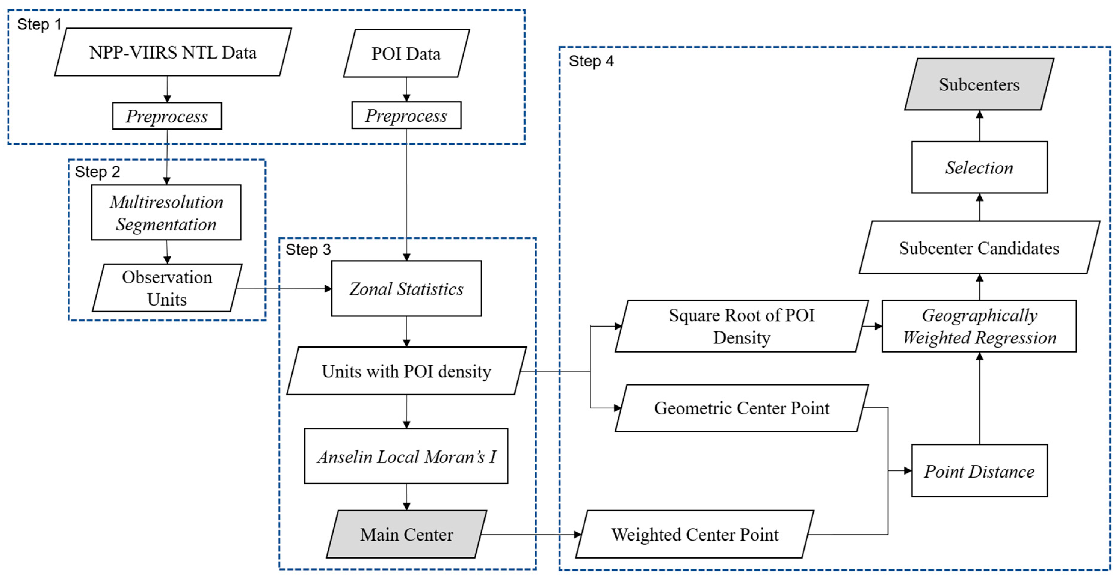
The workflow of the proposed method is shown in Figure 3. First, NPP-VIIRS NTL data and POI data were preprocessed independently. Second, observation units were obtained from the NPP-VIIRS NTL data by multi-resolution segmentation. Next, POI density was calculated by the observation units, and the main center was defined by calculating the Anselin Local Moran’s I. Finally, the subcenters were identified using a geographically weighted regression model according to the square root of POI density and the point distance between the geometric center points of the units and the weighted center point of the main center.

3.1. Data Preprocessing

3.1.1. Preprocessing of NTL Data

The nighttime light image of the study area was extracted using the global VIIRS image and the administrative boundary of study area. In ArcGIS, the monthly average composite night lighting image overlapped with a Google Earth image of the main urban area of Hangzhou, and some easily identified locations, such as the Qiantang River (exhibiting an obvious low gray value) and Xiaoshan International Airport (exhibiting an obvious high gray value), were used as references for registration with the Google Earth image to ensure the accuracy of night image spatial locations.
Because the cloud-free composite products for night lighting did not remove the measurement pixels caused by flashes, gas burning, volcanoes, and auroras or the background noise data caused by low-radiation detection, corresponding processing was needed to filter out such light noise [4]. Theoretically, water pixels have a zero value in the nighttime light data. These could be used as a maximum value to filter the pixels with values under zero. The airport has the runway lights and other high-wattage lighting navigation equipment so the pixels from the airport should have the maximum DN value of the city’s NTL. The filtering process was be conducted in ArcGIS.

3.1.2. Preprocessing of POI Data

A total of 343,064 POI data points were obtained after deduplication, correction, and field investigation verification of the acquired data. Next, the POI data were imported into ArcGIS according to longitude and latitude information and were transformed to the WGS84 projection, for consistency with the NTL data.

3.2. Multi-Resolution Segmentation

To achieve multi-source data fusion and clustering feature analysis, it was necessary to establish a unified spatial unit. Although there were some administrative divisions, human activities are not limited by the administrative boundaries. Therefore, the new statistical units were needed. We used object-based segmentation, by which homogeneous areas with the same spectral or texture features are divided into the same “object”. Nighttime light images were collected by sensors from the real light on the earth’s surface, and the entity objects had different sizes, so the segmentation based on a certain scale could not make good use of its textural features.
Therefore, in our study, we conducted multi-resolution segmentation through multi-resolution models in eCognition, which is the first object-based image analysis commercial software. Multi-resolution segmentation is a bottom-up method [38]. By merging adjacent pixels or small segmentation objects, it accomplishes image segmentation based on region merging technology with the premise of ensuring the maximum average intra-segment heterogeneity and the maximum inter-segment homogeneity [10]. eCognition has the ability to simulate human thinking for image intelligent analysis and information extraction. It supports a variety of image segmentation methods, including chessboard segmentation, quadtree-based segmentation, and multi-resolution segmentation; among these, multi-resolution segmentation is the most commonly used segmentation method. It has three major factors: scale factor, shape factor, and compactness factor.
The segmentation results affected the POI density of each region, and, subsequently, influenced the accuracy of the identified urban center’s spatial extent based on the POI density of those regions. To ensure the accuracy of the experimental results, we selected the optimal parameters of multi-resolution segmentation from the following three aspects.

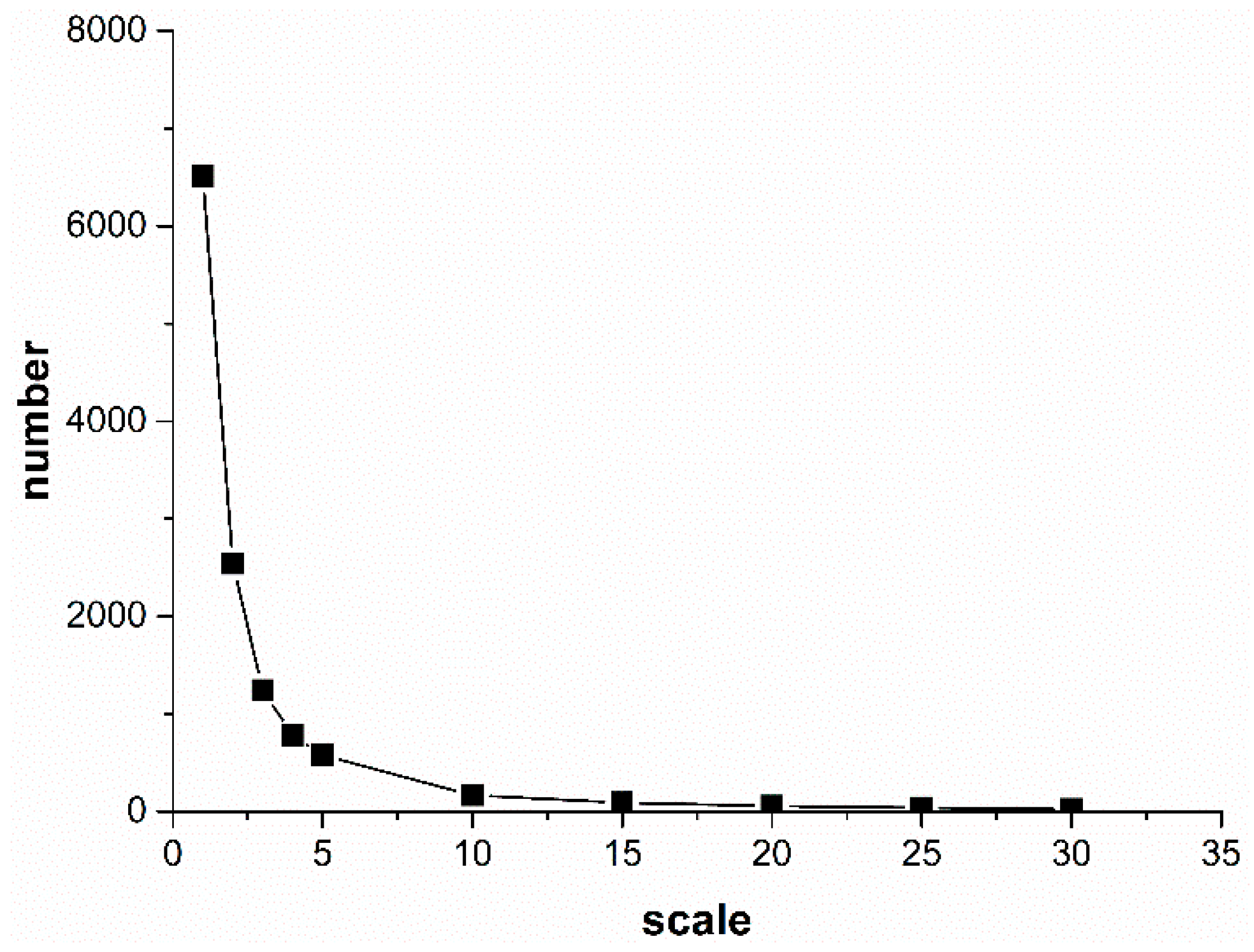
3.2.1. Determination of the Range of the Segmentation Scale Factor

The scale parameter defines the maximum standard deviation of the homogeneity criterion and is the most important factor for the segmentation process. The higher the scale parameter, the larger the object.
Segmentation experiments were carried out on nighttime light images with scale intervals from 1 to 5 and scale ranges from 1–5 to 5–30, and the optimal range of the scale factor was determined according to the relationship between the image segmentation scale and the number of segments (regions) after segmentation. If the number of regions decrease sharply or does not change significantly with an increase in the segmentation scale, the scale factor is not appropriate. If the number of regions change sharply, this indicates that the segmentation is too fragmented and has failed to take advantage of textural features. On the other hand, if the number of regions remain nearly unchanged, this indicates that the segmented units are too full and that the segmentation scale is inappropriate for this case.

3.2.2. Selection of Shape and Compactness Factors

The homogeneity criteria for the multi-resolution segmentation algorithm consist of color and shape factors, with the sum of which is 1. The shape is composed of smoothness and compactness, the sum of these two being 1 [39]. We can set the shape and compactness factors in eCognition. Their values range from 0.1 to 0.9.
To determine the shape and compactness factors, the segmentation scale was selected from the optimal range of the scale factor, and several combinations of the two parameters of shape and compactness were adopted for the segmentation experiment. The optimal combination could be determined through observation by overlaying remote sensing images.

3.2.3. Determination of the Segmentation Scale (Calculated the Weighted Mean Variance)

After determining the parameters of shape and compactness, segmentation experiments were carried out for each scale factor in the optimal range according to Section 3.2.1 to determine the most appropriate segmentation scale parameter for nighttime light images. After the segmentation experiment with the selected scale parameters, the number of segments and the mean value and area of all segments in the segmented image were calculated. Equation (3) was used to calculate the weighted mean variance DN value after segmentation. The scale factor was most appropriate when the variance reached a maximum.
C k ¯ = 1 n i = 1 n C i
C ¯ = 1 m k = 1 m C k ¯
S 2 = 1 m k = 1 m ( C k ¯ C ¯ ) 2
where n is the number of pixels in a segment, C i is the DN value of i th pixel in k th segment, m is the number of segments in the segmented image, and S 2 is the weighted mean variance of DN value in the segmented image.

3.3. Center Detection

3.3.1. Detection of the Main Center

The main center of the city was characterized by clustered plots with high population and activity densities and based on the segmentation result of nighttime light imagery, a spatial clustering analysis method, the Anselin Local Moran’s I, was calculated using the POI density of each unit.
Moran’s I is a common indicator reflecting spatial autocorrelation [40]. Generally, it can be divided into the Global Moran’s I proposed in 1948 and the Anselin Local Moran’s I proposed by professor Luc Anselin from Arizona State University [41]. The former reflects the spatial autocorrelation characteristics of all spatial units, while the latter reflects the spatial autocorrelation strength between a single spatial unit and other spatial units within a defined neighborhood.
To find the main center of Hangzhou, we studied the POI clustering characteristics using the nighttime light data segmentation units. The POI numbers were counted according to the divided areas, the POI density in each plot was calculated, and then Anselin Local Moran’s I (LMI) [42] was applied.
The Anselin Local Moran’s I statistic, I, is defined as follows:
I i = x i x ¯ S i 2 j = 1 , j i n w i j ( x j x ¯ )
where   I i represents the Anselin Local Moran’s I statistics at point i ,   w i j   is the spatial weight matrix,   x i   is the attribute value at point i   ,   x ¯   is the average value of all attribute values, and   S i 2   is:
S i 2 = j = 1 , j i n ( x j x ¯ ) 2 n 1 x ¯ 2
The spatial weight matrix w i j should undergo row normalization,
i = 1 n j i n w i j = n
A z-score, the statistical test for Ii, is as follows,
Z ( I i ) = I i E ( I i ) V a r ( I i )
where E( I i ) is,
E ( I i ) = j = 1 , j i n w i j n 1
Var ( I i ) = E ( I i 2 ) E ( I i ) 2
A high positive value for   I i or   Z ( I i )   ( larger   than   1.96 )   indicates that i is a statistically significant (0.05 level) spatial outlier [10]. According to the significance level of the Anselin Local Moran’s I, the degree of spatial difference between each region and surrounding areas can be divided into two categories by combining the Anselin Local Moran’s I with a Moran scatter diagram. The first type, a high–high agglomeration zone, indicates that the object in this region has a high value and is surrounded by high-value objects. The second type, a low–low agglomeration zone, indicates that the object in this region has a low value and is surrounded by the low value objects. The third type, a high-low agglomeration zone, indicates that the high-value object is surrounded by the low-value objects. The fourth type, a low-high agglomeration zone, indicates that the low value object is surrounded by the high-value objects. The first and second clusters reflect the spatial clustering of similar values, and the third and fourth clusters reflect the spatial clustering of abnormal values.
Through spatial autocorrelation analysis of POI densities, the spatial clustering characteristics of human activities in the study area could be determined. The high–high type block was the main center, and then we found the weighted center of the main center.

3.3.2. Detection of Subcenters

As the main center has the highest level of human activity density, and the subcenter is also a set of contiguous tracts with high levels of human activity density, the subcenter can be defined from two aspects—locally high and globally high. Locally high means that the subcenters have significantly higher densities than their immediate surroundings, while globally high means the relatively high human activity density compared to all of the segments in the study area [10]. Therefore, there was a relationship between the human activity density of subcenters and the distance from the subcenter to the main center. We took the following three steps to identify the subcenters in Hangzhou:
First, we found the geometric center of each unit, and then calculated the distance between each geometric center and the urban center. A geographically weighted regression (GWR) was then calculated using the square root of the POI density and the distance between the plot and the center point. Here, the GWR model is an improved spatial linear regression model. Compared with traditional regression models, this model allows local rather than global parameter estimation and introduces spatial geographic location information from the data [43]. As only nearby observations are used in such estimations, positive residual errors indicate local increases in POI density. Theoretically, if a site is closer to the city-center point, it has more human activity [10]. However, a subcenter is merely a location that has higher local population activity than its surroundings. The expression of the GWR model is given as
y i = β 0 ( μ i , v i ) + j = 1 k β j ( μ i , v i ) x i j + ε i
where y i is the estimated square root of the POI density of segment i; ( μ i , v i )   are the spatial geographic coordinates of segment i; β j ( μ i , v i )   is the jth regression parameter of segment i, and x i j   is the distance from each unit to the city center point. ε i   is the residual error.
We chose the square root of POI density as a dependent variable and the distance from the units to the city center point as an explanatory variable. According to the distribution of factor samples, an adaptive method was used to create the core surface. Finally, plots with standard residuals greater than 1.96 were defined as candidate secondary centers, implying that their POI density values are significantly higher than average at the local scale. Among these, those adjacent to the main center were removed, and the remaining were considered to be secondary centers.

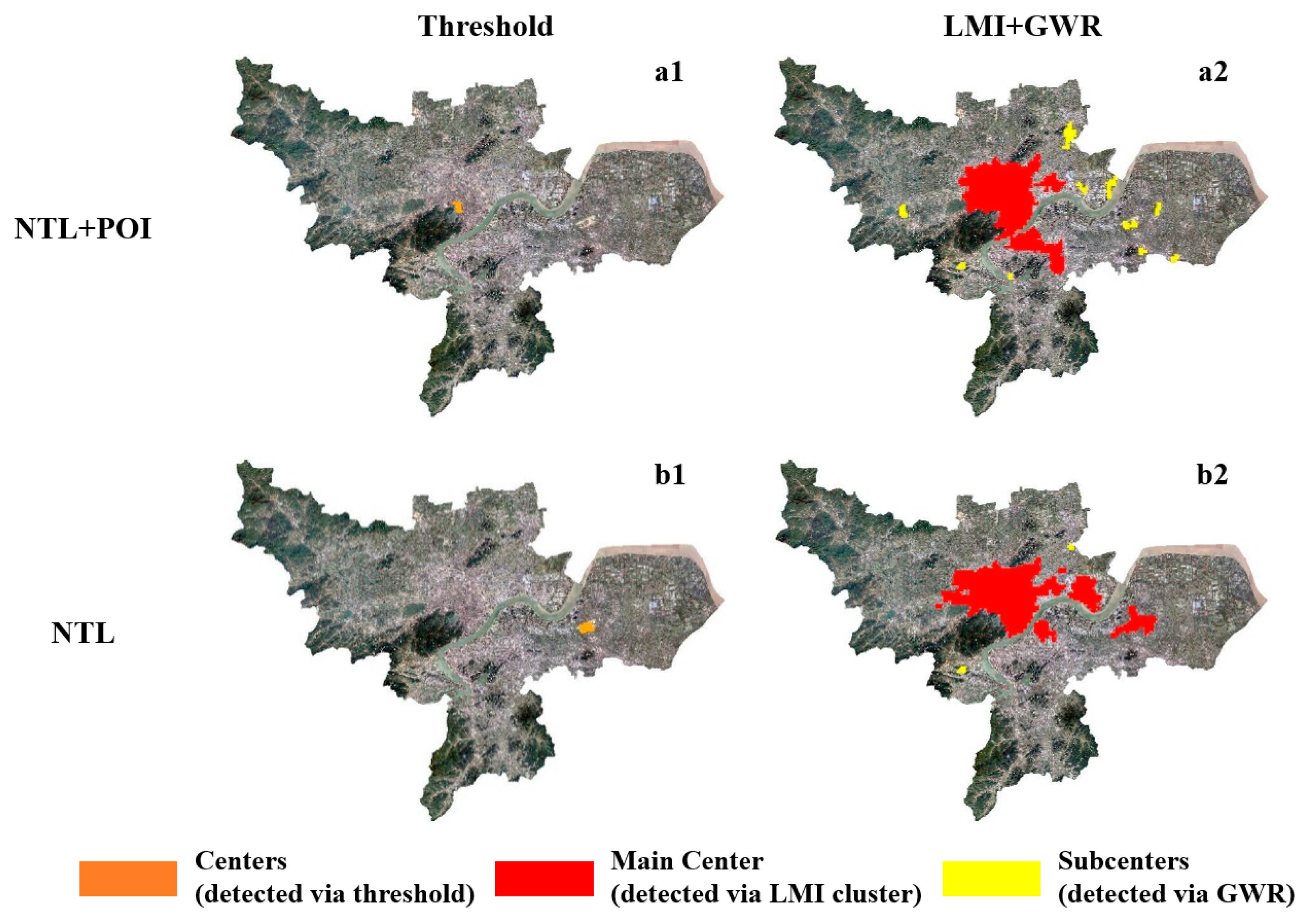
3.4. Comparison Experiment

To verify the accuracy of the proposed method, a threshold method was used for comparison. The mean value of the nighttime light intensity was used as the input for each segmentation unit. We used the relative cut-off threshold method as the comparative method. There are two kinds of threshold methods, one is the absolute threshold method, the other is the relative threshold method. We chose the latter because of its simple implementation and greater objectivity [9] and used 90 percent as the segment threshold according to Liu and Wang [44]. They defined the 90th percentile (selecting the top 10%) of the highest nighttime light intensities by area in China’s megacities as the urban centers.

3.5. Accuracy Assessment

To quantitatively analyze the delineation accuracy of our method and comparison experiments, we evaluated the agreement between the coverage of the detected centers and the coverage of population centers aggregated by population point data. Since the population data represents locations of human beings, such kind of data can be utilized to depict the spatial pattern of human activities. In China, it is always the case that city population centers means city centers especially for those large cities.
Population records were calculated in each grid. We then used hot spot analysis to detect population centers, statistically significant spatial clusters of high values of the analysis results were considered as the referenced center coverage.
We then conducted the confusion matrix in ENVI and used overall accuracy and kappa coefficient to measure the distribution agreement between the city center coverage from population data and the center results.

4. Results

4.1. NTL Data in May 2018 Preprocessing Results

Through observations, the highest light data value at Xiaoshan International Airport was selected as the maximum light threshold (DNmax) used to filter out extremely bright pixel values. For the low-radiation background noise values, we chose sampling points from the area of West Lake in the NPP-VIIRS nighttime light image to record their light values and then utilized their mean value as the minimum light threshold (DNmin). The nighttime light data after processing are shown in Figure 4. The NPP-VIIRS NTL intensity values ranged from 5.51 to 302.99. The red pixels with the highest NTL intensity were located at Xiaoshan Airport. The pixels in the area of the central portion (near West Lake) had higher NTL intensities than those in the marginal areas. In addition, most high intensity pixels (shown in yellow) were concentrated in the northeast part of West Lake and to the banks of the Qiantang River, while the low intensity pixels (shown in blue) were mostly distributed along the border, especially in the northwest, east, and southwest parts of the urban area.

4.2. Multi-Resolution Segmentation Result

In this study, segmentation experiments were carried out on nighttime light images with scale intervals from 1 to 5 and scale ranges from 1–5 to 5–30, and the relationship between the image segmentation scale and the number of segments (regions) after segmentation was obtained, as shown in Figure 5. When the segmentation scale was 1–3, the number of regions decreased sharply with an increase in the segmentation scale. When the segmentation scale was larger than 10, the number of regions did not change significantly with an increase in segmentation scale. Therefore, the range of segmentation scale parameters was determined to be 3–10.
The temporary segmentation scale selected in this study was 5, and nine combinations of the two parameters of shape (0.1,0.5,0.9) and compactness (0.1,0.5,0.9) [39] were used to refer to the segmentation results of a small area in the image.
Superimposed Landsat-8 remote sensing image observations (Figure 6) showed that when the combination was 0.1 and 0.1, the segmentation result of the Qiantang River channel area in the region were too “broken”. When combinations of 0.5 and 0.9, 0.9 and 0.5, or 0.9 and 0.9 were used, the contour of the dividing line near the river course in the region was beyond the actual boundary, and the proportions of land and water in part of the segmentation unit were equal, and the segmentation result was flooded. When the combinations were 0.5 and 0.5, 0.9 and 0.1, or 0.5 and 0.1, the flooding phenomenon was more severe, and the river was almost completely undistinguishable from its surroundings, such as the green land and construction land.
The segmentation results of the combinations 0.1 and 0.5 and 0.1 and 0.9 showed better results. Because the segmentation results of the two combinations were relatively close, the shape parameter selected in this paper was 0.1 and the compactness parameter was 0.5.
Based on the 0.1 shape factor and 0.5 compactness factor, segmentation experiments were carried out at 5 scales, including scale 3, 4, 5, 6, 7, and 8, to determine the optimal segmentation scale parameters for nighttime light images. Figure 7 shows the relationship between the weighted mean variances of segments and the segmentation scale.
Finally, a scale factor of 6, shape of 0.1, and compactness of 0.5 were selected for multi-resolution segmentation. The segments were exported as a shape file and converted to the WGS84 projection in ArcGIS. Areas that were too small resulted in POI densities that were unrealistically high. Therefore, fusion processing was carried out for units less than 1 km2 using the eliminate tool in ArcGIS.
Utilizing a multi-resolution segmentation algorithm, a total of 402 segments were obtained. After elimination of the small segments, 358 remained. Figure 8 shows the POI density of each segment. The classification method of the color ramp used natural breaks. This was done so that the differences between classes were maximized and that the areas of each color were well proportioned. It was found that the central area (near West Lake) had smaller units than those in the marginal areas. In addition, the red and orange parts with higher POI densities were concentrated in the northeast part of West Lake and to the banks of the Qiantang River, while the green parts with low POI densities were mostly distributed along the border, especially in the northwest, east, and southwest parts of the urban area.

4.3. Center Detection Results

4.3.1. Main Centers

In the study, the weight matrix was determined by inverse-distance method. It means that nearby neighboring features have a larger influence on the computations for a target feature than features that are far away. And then a row standardization was conducted. It means that spatial weights were standardized and each weight was divided by its row sum. The results of local spatial autocorrelation analysis with the spatial units and the statistics of each cluster segmentation are shown in Figure 9. The units with a clustering type of “high–high” were regarded as the main centers. They contained 152,643 pieces of POI data, accounting for 44.5% of the total POI. As Figure 10 shows, the main centers of Hangzhou were located in the middle of the study area and the Qiantang River runs through them.

4.3.2. Subcenters

After geographically weighted regression (GWR), there were 14 units with standard residual errors greater than 1.96. The adjacent units were combined into a secondary center area, and 13 candidate subcenters were obtained. After removing three of them, which were within, adjacent to, or intersecting, ten subcenters were finally obtained. The total area of the subcenters was 41.15 km2.

4.4. Comparison Experiment Results

Figure 11 shows the results of the comparison experiment. The results of the threshold are shown in orange. By counting the POI numbers inside each nighttime light (NTL) segment, there was only one unit with a POI density over 90 percent (a1). When the data source was NTL, the threshold method resulted in a city center located at the Xiaoshan Airport (b1) because the airport runway lights and other high-wattage lighting navigation equipment caused the region to show extremely high brightness values in the nighttime remote sensing image. This was clearly not very practical. The airport would not be considered the main city center due to its large population mobility and unitary regional functions. The results of our method with NTL (b2) were similar to the experimental results (a2). However, these results showed more parts in the main center and fewer parts in the subcenters. Our method detected two main centers and ten subcenters, while there were only two subcenters located in the Linping and Yuhang district, that were detected in b2. Furthermore, the area around the airport was detected as the main center. Therefore, it was found that the POI data source was indispensable.

4.5. Accuracy Assessment Results

The population data were calculated in the grids of 500 m. The population hot spot map is shown in Figure 12. The map shows that the population were mainly clustering at the central part of the study area. The hot spot areas and cold spot areas were separated by not significant areas. There are more cold spot areas than hot spots near the border.
We chose the hot spot areas with 95% confidence as the reference centers. Based on the comparison experiment results, the intersect analysis were conducted using population centers. Figure 13 shows the comparison of four results and population centers. The center areas that were detected by both were shown in green and the different center areas were shown in gray.
The accuracy assessment results were shown in Table 1. It could be found that the results of the combination of nighttime light data and POI data under LMI and GWR were better than others.

5. Discussion

To verify the effectiveness of the multicenter identification results of our method, we compared the experimental results with the urban center system proposed in the current Hangzhou City Master Plan Evaluation Report (hereinafter referred to as Report).
The Report evaluates the implementation of various aspects of the plan, such as the transportation system, industry, and ecological environment. According to the master plan, the urban spatial structure of Hangzhou develops from a single center around West Lake to a multicenter structure with group sets, forming an open spatial structure of “One main, three pairs, two centers and two axes, six groups and six ecological belts” [45]. In addition, three subcenters of Dajiangdong New City, Chengbei New City and Future Science and Technology City were added to the level of the urban public service center, to optimize and adjust the multi-center system at the urban macro scale [46].
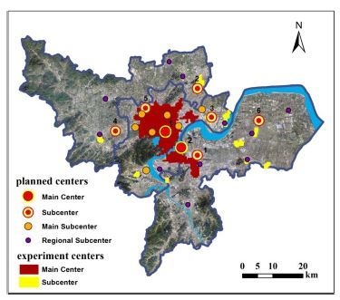
In Chapter 6 of the Report, the spatial pattern assessment, the implementation of urban centers was evaluated according to the master plan, and was expressed by stars, ranging from one star to five stars. The locations of the centers are shown in Figure 14. The Report notes out that the main center has basically reached the standard, while there are gaps in the construction of the subcenters (Table 2).

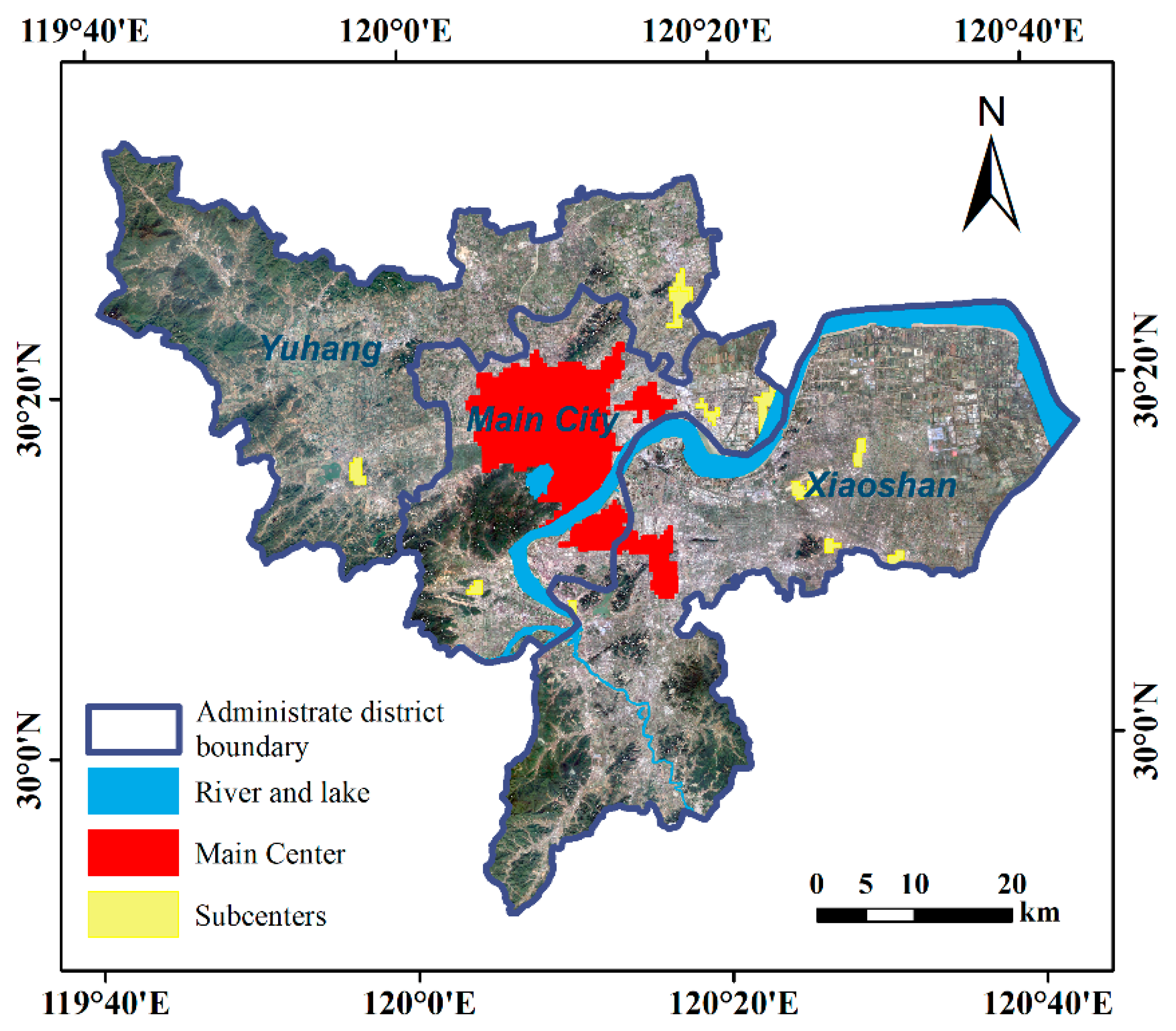
5.1. Comparison of Main Centers and Analysis

Through the comparison, it was found that the two main centers in the plan were consistent with the experimental results in this paper: Yan’an Road and the area near West Lake on the north side of the river, and Qianjiang new town and Qianjiang century city were shown to the south of the river. However, the southeast part of the main center area in our experimental results extended outward more than expected, covering the Jiangnan City Center, located to the southeast of the main center area in the Plan.
As mentioned in the evaluation of subcenters in the Report, three of the six subcenters were well implemented, including the Jiangnancheng subcenter. Therefore, we can consider that our experimental results are consistent with the facts.

5.2. Comparison of Subcenters and Analysis

The polycentric system is divided into three levels in the master plan and evaluation report: the main center, the subcenter and the tertiary center. However, this paper only studied the central system for two levels, so we combined the subcenters and the tertiary center in the Report and compared them with the subcenters in our results.
Our method identified nearly all of the subcenters appearing in the Report, and the only one not identified was the Yuhang Group Center. The Yipeng Group Center was identified, but its position was slightly inaccurate. This was probably because the state of planning implementation in this area was poor, so there might be insufficient infrastructure and low population density. At the same time, the center we identified was located on the southwestern side of this planning point, and it was closer to a tertiary center called the Airport Subcenter. Two subcenters in the plan, Xiasha City Center and Liangzhu Group Center, were identified by us within the scope of the main center.
The tertiary centers in the Report contained two types, third grade centers and fourth grade centers (Figure 14). We identified two-thirds of these, and all main subcenters that we identified were within the main centers. This was in agreement with the plan.

6. Conclusions

In this study, the city centers of Hangzhou were detected using a combination of two types of data, including open-net POI maps and nighttime light images with high spatial resolutions. The results from different data sources and methods were compared and the accuracy and rationality of the proposed method were demonstrated. The major findings of this study were as follows: (1) An optimal multi-resolution segmentation parameter combination was found; (2) the main centers and subcenters were detected and showed clear boundaries; and (3) the proposed method that combined nighttime light data and POI data could effectively detect urban centers. This method provided a new way to identify the urban spatial structure and could be applied to the evaluation of urban development.
There are several characteristics of POI that are related to the boundaries of urban centers, in addition to the number and density, for example, the scale of an area, the usage rate, the relationships with human activities, and the used ages. In this study, the spatial patterns of POI were the focus. Therefore, in the future, other characteristics of POI data might be used to more precisely measure the boundaries of city centers when combined with nighttime light data.

Author Contributions

Conceptualization, G.L., Q.C. and Z.S.; Methodology, G.L., Q.C. and K.H.; Software, G.L. and Y.Z.; Formal analysis, G.L., Q.C. and Z.S.; Investigation, G.L. and Y.Z.; Resources, G.L., Q.C. and Z.S.; Data curation, G.L. and Q.C.; Writing—original draft preparation, G.L., Q.C. and Z.S.; Writing—review and editing, G.L., Q.C., Z.S., K.H. and Y.Z.; Visualization, G.L., K.H. and Y.Z.; Supervision, Q.C., Z.S. and K.H.; Project administration, Q.C. and Z.S.; Funding acquisition, Q.C. and Z.S.

Funding

This study was financially supported by the Fundamental Research Funds for the Central Universities (2019FZA6005), International S&T Cooperation Program of China (2010DFA92720-27) and National key research and development program of China (2018YFD1100302-04).

Acknowledgments

The authors would like to thank the staff of MDPI for language editing, editors and the anonymous reviewers for their constructive comments which have been very helpful in revising this paper.

Conflicts of Interest

The authors declare no conflict of interest.

References

  1. Definitions of Urban Center. Available online: https://www.vocabulary.com/dictionary/urban%20center (accessed on 30 July 2019).
  2. Sun, B.; Shi, W.; Ning, Y. An empirical study on the polycentric urban structure of Shanghai and strategies in future. Urban Plan. Forum 2010, 1, 58–63. [Google Scholar]
  3. Xie, Z.W.; Ye, X.Y.; Zheng, Z.H.; Li, D.; Sun, L.S.; Li, R.R.; Benya, S. Modeling polycentric urbanization using multisource big geospatial data. Remote Sens. 2019, 3, 310. [Google Scholar] [CrossRef]
  4. Tang, C. Improvement of urban construction land extraction method based on NPP-VIIRS nighttime light data and landsat-8 data: A case study of Guangzhou city. Geomat. Spat. Inf. Technol. 2017, 40, 69–73. [Google Scholar]
  5. Marzena, W.; Monika, K. The continuous built-up area extracted from ISS night-time lights to compare the amount of urban green areas across European cities. Eur. J. Remote Sens. 2019, 52, 58–73. [Google Scholar] [CrossRef]
  6. Elvidge, C.D.; Baugh, K.E.; Kihn, E.A.; Kroehl, H.W.; Davis, E.R. Mapping city lights with nighttime data from the DMSP operational linescan system. Photogramm. Eng. Remote Sens. 1997, 63, 727–734. [Google Scholar]
  7. Miller, S.D.; Straka, W.; Mills, S.P.; Elvidge, C.D.; Lee, T.F.; Solbrig, J.; Walther, A.; Heidinger, A.K.; Weiss, S.C. Illuminating the capabilities of the Suomi national polar-orbiting partnership (NPP) visible infrared imaging radiometer suite (VIIRS) day/night band. Remote Sens. 2013, 5, 6717–6766. [Google Scholar] [CrossRef]
  8. Ma, T.; Yin, Z.; Zhou, A. Delineating spatial patterns in human settlements using VIIRS nighttime light data: A watershed-based partition approach. Remote Sens. 2018, 10, 465. [Google Scholar] [CrossRef]
  9. Small, C.; Pozzi, F.; Elvidge, C. Spatial analysis of global urban extent from DMSP-OLS night lights. Remote Sens. Environ. 2005, 96, 277–291. [Google Scholar] [CrossRef]
  10. Cai, J.; Huang, B.; Song, Y. Using multi-source geospatial big data to identify the structure of polycentric cities. Remote Sens. Environ. 2017, 202, 210–221. [Google Scholar] [CrossRef]
  11. Zheng, Q.; Jiang, R.; Wang, K.; Huang, L.; Ye, Z.; Gan, M.; Ji, B. Monitoring the trajectory of urban nighttime light hotspots using a Gaussian volume model. Int. J. Appl. Earth Obs. Geoinf. 2018, 65, 24–34. [Google Scholar] [CrossRef]
  12. Huang, X.; Wen, D.; Li, J.; Qin, R. Multi-level monitoring of subtle urban changes for the megacities of China using high-resolution multi-view satellite imagery. Remote Sens. Environ. 2017, 196, 56–75. [Google Scholar] [CrossRef]
  13. Li, X.; Xu, H.; Chen, X.; Li, C. Potential of NPP-VIIRS Nighttime Light Imagery for Modeling the Regional Economy of China. Remote Sens. 2013, 5, 3057–3081. [Google Scholar] [CrossRef] [Green Version]
  14. Ma, T.; Zhou, C.; Pei, T.; Haynie, S.; Fan, J. Quantitative estimation of urbanization dynamics using time series of DMSP/OLS nighttime light data: A comparative case study from China’s cities. Remote Sens. Environ. 2012, 124, 99–107. [Google Scholar] [CrossRef]
  15. Zhao, X.; Yu, B.; Liu, Y.; Yao, S.; Lian, T.; Chen, L.; Yang, C.; Chen, Z.; Wu, J. NPP-VIIRS DNB daily data in natural disaster assessment: Evidence from selected case studies. Remote Sens. 2018, 10, 1526. [Google Scholar] [CrossRef]
  16. Paulino, C.; Aroni, E.; Xu, H.; Alburqueque, E.; Demarcq, H. Use of nighttime visible images in the study of the spatial and temporal variability of fishing areas of jumbo flying squid (Dosidicus gigas) outside Peruvian EEZ 2004–2015. Fish. Res. 2017, 191, 144–153. [Google Scholar] [CrossRef]
  17. Waluda, C.M.; Trathan, P.N.; Elvidge, C.D.; Hobson, V.R.; Rodhouse, P.G. Throwing light on straddling stocks of Illex argentinus: Assessing fishing intensity with satellite imagery. Can. J. Fish. Aquat. Sci. 2002, 59, 592–596. [Google Scholar] [CrossRef]
  18. Ji, G.; Tian, L.; Zhao, J.; Yue, Y.; Wang, Z. Detecting spatiotemporal dynamics of PM2.5 emission data in China using DMSP-OLS nighttime stable light data. J. Clean. Prod. 2019, 209, 363–370. [Google Scholar] [CrossRef]
  19. Zhao, N.; Cao, G.; Zhang, W.; Samson, E.L. Tweets or nighttime lights: Comparison for preeminence in estimating socioeconomic factors. ISPRS J. Photogramm. Remote Sens. 2018, 146, 1–10. [Google Scholar] [CrossRef]
  20. Anderson, S.J.; Tuttle, B.T.; Powell, R.L.; Sutton, P.C. Characterizing relationships between population density and nighttime imagery for Denver, Colorado: Issues of scale and representation. Int. J. Remote Sens. 2010, 31, 5733–5746. [Google Scholar] [CrossRef]
  21. Yu, B.; Shi, K.; Hu, Y.; Huang, C.; Chen, Z.; Wu, J. Poverty evaluation using NPP-VIIRS nighttime light composite data at the county level in China. IEEE J. Sel. Top. Appl. Earth Obs. Remote Sens. 2015, 8, 1217–1229. [Google Scholar] [CrossRef]
  22. Elvidge, C.D.; Baugh, K.E.; Zhizhin, M.; Hsu, F.C. Why VIIRS data are superior to DMSP for mapping nighttime lights. Proc. Asia-Pac. Adv. Netw. 2013, 35, 62. [Google Scholar] [CrossRef] [Green Version]
  23. Liu, X.; Wang, J. The geography of Weibo. Environ. Plan. A Econ. Space 2015, 47, 1231–1234. [Google Scholar] [CrossRef] [Green Version]
  24. Yao, Y.; Li, X.; Liu, X.; Liu, P.; Liang, Z.; Zhang, J.; Mai, K. Sensing spatial distribution of urban land use by integrating points-of-interest and Google Word2Vec model. Int. J. Geogr. Inf. Sci. 2016, 31, 825–848. [Google Scholar] [CrossRef]
  25. Zheng, X. Identification and optimization of Xi’an urban center system based on open data. Planners 2017, 1, 57–64. [Google Scholar]
  26. Jia, Y.; Ge, Y.; Ling, F.; Guo, X.; Wang, J.; Wang, L.; Chen, Y.; Li, X. Urban land use mapping by combining remote sensing imagery and mobile phone positioning data. Remote Sens. 2018, 10, 446. [Google Scholar] [CrossRef]
  27. Chen, Y.; Ge, Y.; An, R.; Chen, Y. Super-resolution mapping of impervious surfaces from remotely sensed imagery with points-of-interest. Remote Sens. 2018, 10, 242. [Google Scholar] [CrossRef]
  28. Long, Y.; Shen, Y.; Jin, X. Mapping block-level urban areas for all Chinese cities. Ann. Am. Assoc. Geogr. 2015, 106, 96–113. [Google Scholar] [CrossRef]
  29. Li, K.; Chen, Y.; Li, Y. The random forest-based method of fine-resolution population spatialization by using the international space station nighttime photography and social sensing data. Remote Sens. 2018, 10, 1650. [Google Scholar] [CrossRef]
  30. Yao, Y.; Liu, X.; Li, X.; Zhang, J.; Liang, Z.; Mai, K.; Zhang, Y. Mapping fine-scale population distributions at the building level by integrating multisource geospatial big data. Int. J. Geogr. Inf. Sci. 2017, 31, 1220–1244. [Google Scholar] [CrossRef]
  31. Duan, Y.; Liu, Y.; Liu, X.; Wang, H. Identification of polycentric urban structure of central Chongqing using points of interest big data. J. Nat. Res. 2018, 33, 788–800. [Google Scholar] [CrossRef]
  32. Wu, K.; Zhang, H.; Wang, Y.; Wu, Q.; Ye, Y. Identification and spatial pattern of Guangzhou multi-type commercial center. Progr. Geogr. 2016, 35, 963–974. [Google Scholar] [CrossRef]
  33. Guo, J.; Lv, Y.; Shen, T. Urban Spatial structure based on point pattern analysis—taking beijing metropolitan area as a case. Econ. Geogr. 2015, 35, 68–74. [Google Scholar] [CrossRef]
  34. Pan, S. Spatial coupling between housing development and economic growth based on night light remote sensing and residential POI. J. Geo-Inf. Sci. 2017, 19, 646–652. [Google Scholar] [CrossRef]
  35. Yu, B.; Liu, Y.; Chen, G. Urban spatial structure of port city in South China Sea based on spatial coupling between nighttime light data and POI. J. Geo-Inf. Sci. 2018, 20, 854–861. [Google Scholar] [CrossRef]
  36. Zhang, S.; Tang, J.; Wang, H.; Wang, Y.; An, S. Revealing intra-urban travel patterns and service ranges from taxi trajectories. J. Trans. Geogr. 2017, 61, 72–86. [Google Scholar] [CrossRef]
  37. Bennett, M.M.; Smith, L.C. Advances in using multitemporal night-time lights satellite imagery to detect, estimate, and monitor socioeconomic dynamics. Remote Sens. Environ. 2017, 192, 176–197. [Google Scholar] [CrossRef]
  38. Kohli, D.; Warwadekar, P.; Kerle, N.; Sliuzas, R.; Stein, A. Transferability of object-oriented image analysis methods for slum identification. Remote Sens. 2013, 5, 4209–4228. [Google Scholar] [CrossRef]
  39. Wang, Z.; Chen, G.; Yu, B.; Zhang, X. Determination of the optimal segmentation scale of high-resolution remote sensing images of islands and reefs in the south China sea. Geosptial Inf. 2018, 16, 21–24. [Google Scholar]
  40. Deng, M.; Liu, Q. Spatial Analysis; Surveying and Mapping Press: Beijing, China, 2015. [Google Scholar]
  41. Su, L.Y.; Yang, X.H.; Bai, G.Y.; Li, F.L. Spatial inequality and regional difference of population birth rate in China. J. Chongqing Univ. Technol. 2018, 32, 249–258. [Google Scholar]
  42. Anselin, L. Local indicators of spatial association-LISA. Geogr. Anal. 1995, 27, 93–115. [Google Scholar] [CrossRef]
  43. Yin, S.; Song, W.; Ma, Z.; Li, Z.; Wu, Q. Spatial differentiation and influencing factors analysis of housing prices in Nanjing: Based on geographically weighted regression model. Hum. Geogr. 2018, 33, 68–77. [Google Scholar] [CrossRef]
  44. Liu, X.; Wang, M. How polycentric is urban China and why? A case study of 318 cities. Landsc. Urban Plan. 2016, 151, 10–20. [Google Scholar] [CrossRef]
  45. Zhang, L.; Yue, W.; Liu, Y. Multidimensional analysis of the polycentric urban spatial structure—A case of Hangzhou. Econ. Geogr. 2017, 37, 67–75. [Google Scholar] [CrossRef]
  46. Wu, Q.; Liu, X. Study on urban polycentricity of Hangzhou based on service facilities. Mod. Urban Res. 2018, 10, 28–36. [Google Scholar]
Figure 1. Location of the study area. The inset map shows the location of Hangzhou in Zhejiang province.
Remotesensing 11 01821 g001
Figure 2. Point of interest (POI) data of Hangzhou in May 2018: (a) Spatial distribution of POI, each point stands for one point of interest. (b) Gridded map of POI number with 500 m resolution, representing the number of POI in a square of 25 ha.
Remotesensing 11 01821 g002
Figure 3. Workflow of the proposed method. NTL: nighttime light; NPP-VIIRS: visible infrared imaging radiometer suite.
Remotesensing 11 01821 g003
Figure 4. NPP-VIIRS nighttime light intensity map of Hangzhou in May 2018. (NPP-VIIRS: Suomi-NPP satellite, visible infrared imaging radiometer).
Remotesensing 11 01821 g004
Figure 5. of segments changes with segmentation scale factor using multi-resolution segmentation in eCognition.
Remotesensing 11 01821 g005
Figure 6. Segmentation results of nine groups of shape factor and compactness factor combinations (here shows a small region). The yellow lines show the boundaries of segments. The image with red frame means the factor combination we chose to use (shape factor is 0.1 and compactness factor is 0.5).
Remotesensing 11 01821 g006
Figure 7. Weighted mean variances of segments for different scale factors (3,4,5,6,7,8).
Remotesensing 11 01821 g007
Figure 8. Density of POI counted in segmentation units. The small images on the right show detailed views of the areas of small units and big units respectively.
Remotesensing 11 01821 g008
Figure 9. Four cluster types of the results of local spatial autocorrelation analysis for the POI densities in units.
Remotesensing 11 01821 g009
Figure 10. Main centers and subcenters detected by the proposed method. The main centers are shown in red, and the subcenters are shown in yellow. The river and lake layer contains West Lake and the Qiantang River.
Remotesensing 11 01821 g010
Figure 11. Centers detected by different methods and datasets. All centers detected by threshold are shown in orange. In the results from the Local Moran’s I (LMI) and geographically weighted regression (GWR) methods, the main centers are shown in red, and the subcenters are shown in yellow.
Remotesensing 11 01821 g011
Figure 12. Hot spot analysis result of population data.
Remotesensing 11 01821 g012
Figure 13. Centers areas intersect results. The overlapped center areas were shown in green and the different center areas were shown in gray.
Remotesensing 11 01821 g013
Figure 14. Centers proposed in the master plan and detected by our experiment.
Remotesensing 11 01821 g014
Table 1. Overall accuracy (OA) and kappa coefficient of four types of results.
DataThresholdLMI+GWR
OAKappaOAKappa
NTL+POI84.9228%0.009490.8185%0.5546
NTL84.7039%−0.001788.9350%0.4692
Table 2. Evaluation of the central system from the Report (excerpts).
ClassNumberNameDegree of Implementation
Municipal centerMain center1Yan‘an Road and the area near West Lake★★★★★ *
2Qianjiang New Town and Qianjiang Century CityQianjiang new town ★★★★★
Qianjiang century city ★★★☆☆
Municipal subcentersubcenter1Jiangnan City Center★★★★☆
2Linping City Center★★★★☆
3Xiasha City Center★★☆☆☆
4Yuhang Group Center★★★★☆
5Liangzhu Group Center★★★★☆
6Yipeng Group Center★★☆☆☆
*: The stars express the degree of implementation. One star and five stars correspond to the lowest and the highest degree of implementation respectively.

