From Archived Historical Aerial Imagery to Informative Orthophotos: A Framework for Retrieving the Past in Long-Term Socioecological Research

Abstract

Aerial photographs have been systematically collected from as early as the 1930s, providing a unique resource to describe changes in vegetation and land cover over extended periods of time. However, their use is often limited by technical constraints, such as the lack of ground control information and precise camera parameters, which hamper an accurate orthorectification of the raw imagery. Here, we describe the historical aerial photographs orthorectification (HAPO) workflow, based on a conventional photogrammetric procedure (the direct linear transformation (DLT) Method), integrated as a geographic information systems (GIS) procedure, in order to perform the image orientation and orthorectification, thereby converting historical aerial imagery into high-definition historical orthoimages. HAPO implementation is illustrated with an application to a rugged landscape in Portugal, where we aimed to produce land-cover maps using an aerial photograph coverage from 1947, as part of a study on long-term socioecological dynamics. We show that HAPO produces highly accurate orthoimages and discuss the wider usefulness of our framework in long-term socioecological research.

1. Introduction

Historical aerial photographs (HAP) are the oldest form of remotely sensed data, yielding a spectrum of valuable historical information on vegetation and land cover [1,2,3]. Such information has enormous potential to provide crucial baseline data for quantitative mapping and monitoring of landscape composition and heterogeneity over time [3,4,5,6,7,8,9], and to relate land-use history to changes in biodiversity and ecosystem services [2,10,11,12]. Aerial photographs started to be produced from as early as the 1930s [1,9], whereas satellite imagery only became available in the 1970s and, at the beginning, had coarse spatial resolution [9,13], which limits their usefulness to analyze long-term landscape change. Despite their value, however, the potential of HAP remains clearly underexplored due in part to technical constraints [14], thus hindering a thorough understanding of the spatial and temporal patterns of land use and land cover, and their resulting environmental impacts, particularly during the pre-satellite era [12].

The use of HAP is challenging due to the need for accurately georeferencing the photos to a ground coordinate system, so they can be compared with other geographic datasets in geographic information systems (GIS) [2,15,16,17,18]. In general, GIS users do not have easy access to photogrammetry software tools. Additionally, HAP orthorectification is a complex and difficult process since historical ground control information, calibration certificates, and precise or even basic knowledge of camera parameters are often not available [16,17,18,19]. Furthermore, processing HAP presents additional challenges in landscapes undergoing regime shift processes [2,16,17,18,19], due to the dramatic land-cover changes that can occur over time [20], making it difficult to find adequate ground control features that can be georeferenced from information in modern orthoimages. Probably because of these problems, to our knowledge, there is still no fully automatic pipeline for generating orthoimages from HAP [14].

To address these challenges, some studies have exploited a relatively fast and semiautomatic process by using the implicit depth information contained in overlapping imagery, and by subsequently introducing the extracted digital surface model (DSM) information into an object-based image analysis (OBIA) process (e.g., [18,21]). However, automatic extraction of DSMs with image-matching algorithms can deliver undesirable results (spiky surface models), resulting from unmodeled distortions, errors in the interior orientation parameters, and/or low radiometric quality [19]. Moreover, historical aerial stereo pairs are often not available, due to deterioration by age or other circumstances, as relocations or accidents in the archive facilities (e.g., [15]), which can damage part of the collections. Further, this approach cannot be used in the case of isolated images or incomplete data sets.

To overcome these problems, we developed a new workflow providing accurate historical aerial photographs orthorectification (HAPO) and georeferencing, which is implemented through a program we called “Projective 3D” (PRJ3D). GIS software, such as ArcGIS or QGIS, implements the projective transformation as a 2D image georeferencing method, which is only suitable for aerial photographs of flat terrain. Our method brings the third dimension into the process, combining direct linear transformation (DLT) for an individual image orientation, and conventional photogrammetric orthorectification procedures with a digital elevation model (DEM) for resampling individual historical aerial imagery into high-definition historical orthoimages. The methodology brings the old DLT method, normally not used in photogrammetric software tools, into an image-georeferencing process, overcoming the limitations found by GIS users in dealing with HAP. In this study, we describe the HAPO workflow, detailing all the steps required to process isolated or marginally overlapping sets of HAP. Workflow implementation is illustrated with a case study in Portugal, where we aimed to produce land-cover maps using aerial photograph coverage from 1947. The study shows the potential of HAPO to solve problems commonly encountered when orthorectifying historical aerial photographs and underlines its potential wide applicability in similar studies addressing long-term landscape dynamics.

2. Background

Aerial photographs have been systematically collected over decades for producing military and civilian maps and are archived in many institutions worldwide [15,22]. This resource has been used in a number of scientific fields, and its importance has increased in recent years to address questions involving long-term changes in socioecological systems. This is shown, for instance, by a simple literature search performed in ISI Web of Science (in December 2018), covering the period 1990–2018, where we used the search string TS = (“historical aerial photographs*” OR “Orthorectification* historical aerial photographs*” OR “historical imagery*” OR “orthorectification* historical imagery*” OR “historical photography*” OR “orthorectification* historical photography*”). The 260 papers retrieved by this search were spread over different research topics, such as geosciences (78 papers), geography (61), remote sensing (24), and environmental sciences/ecology (97), and there was a steady increase in the number of papers published since the 1990s (19) until the 2010s (241). Most studies using HAP in environmental/ecology applications were carried out in the USA (50%), while European studies represented a smaller proportion (29%).

These previous studies have used several different approaches to extract information from HAP. Some studies used a simple approach involving only HAP relative image orientation rather than georeferencing and orthorectification [15,19,23,24,25,26], which provides a quick solution when a coarse spatial resolution is sufficient to detect changes [27,28]. These studies generally addressed stable areas over time, usually urban or man-constructed features [2], with analyses of change usually carried out over small spatial extents or at low resolutions. Other studies retrieved from the literature search used previously orthorectified (e.g., [9,29]) or only georeferenced (e.g., [30,31,32]) images but provided little information on image processing. In other cases, the camera information (metadata) was complete and available (e.g., [33,34,35]), but often there was no reference to the orthorectification process itself (e.g., [36,37,38,39]). More detail is usually given in technical studies dealing specifically with remote sensing, with several authors describing feature-based registration methodologies for historical aerial image orientation and orthorectification, such as the use of TIL (time-invariant lines) (e.g., [17]) or OBIA processes (e.g., [21]). However, the application of a standard bundle adjustment [16,18,19,36] is not possible when only even or odd HAP along strips are available, because the marginal overlap is around 20% and not the standard 60% of stereo pairs.

Overall, there are still significant technical constraints to retrieve meaningful information from HAP. Such constraints are particularly challenging when HAP are to be used in long-term socioecological studies, for which coarse thematic (and spatial) resolution classification systems may be insufficient to describe and understand the patterns and processes of landscape change [40]. For instance, these studies often require the identification of small patches or region-specific habitats of particular ecological importance [41], and to map their distribution at the landscape scale is not possible when using simple approaches, such as relative HAP orientation. Therefore, methods are still needed to deal successfully with the challenges of accurate HAP orthorectification, and to retrieve fine-scale information essential for high-resolution, spatially explicit long-term socioecological reconstructions [3]. In this paper, we address the main challenges of HAP georeferencing and orthorectification, describing a new workflow (HAPO) that can be used in the absence of ground control information or camera calibration and can be applied to isolated HAP or when stereo pairs are unavailable.

3. Methods

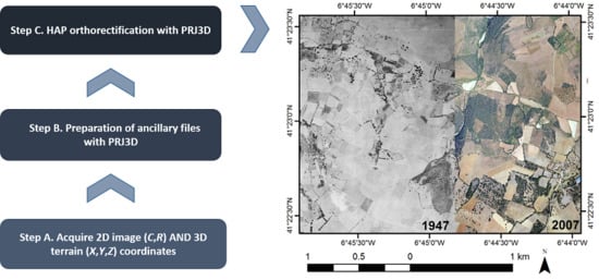
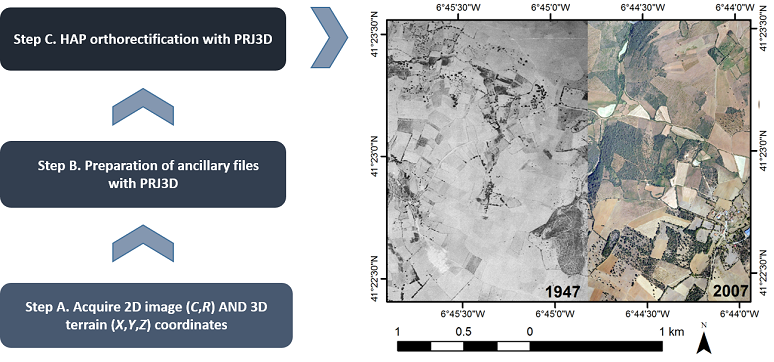
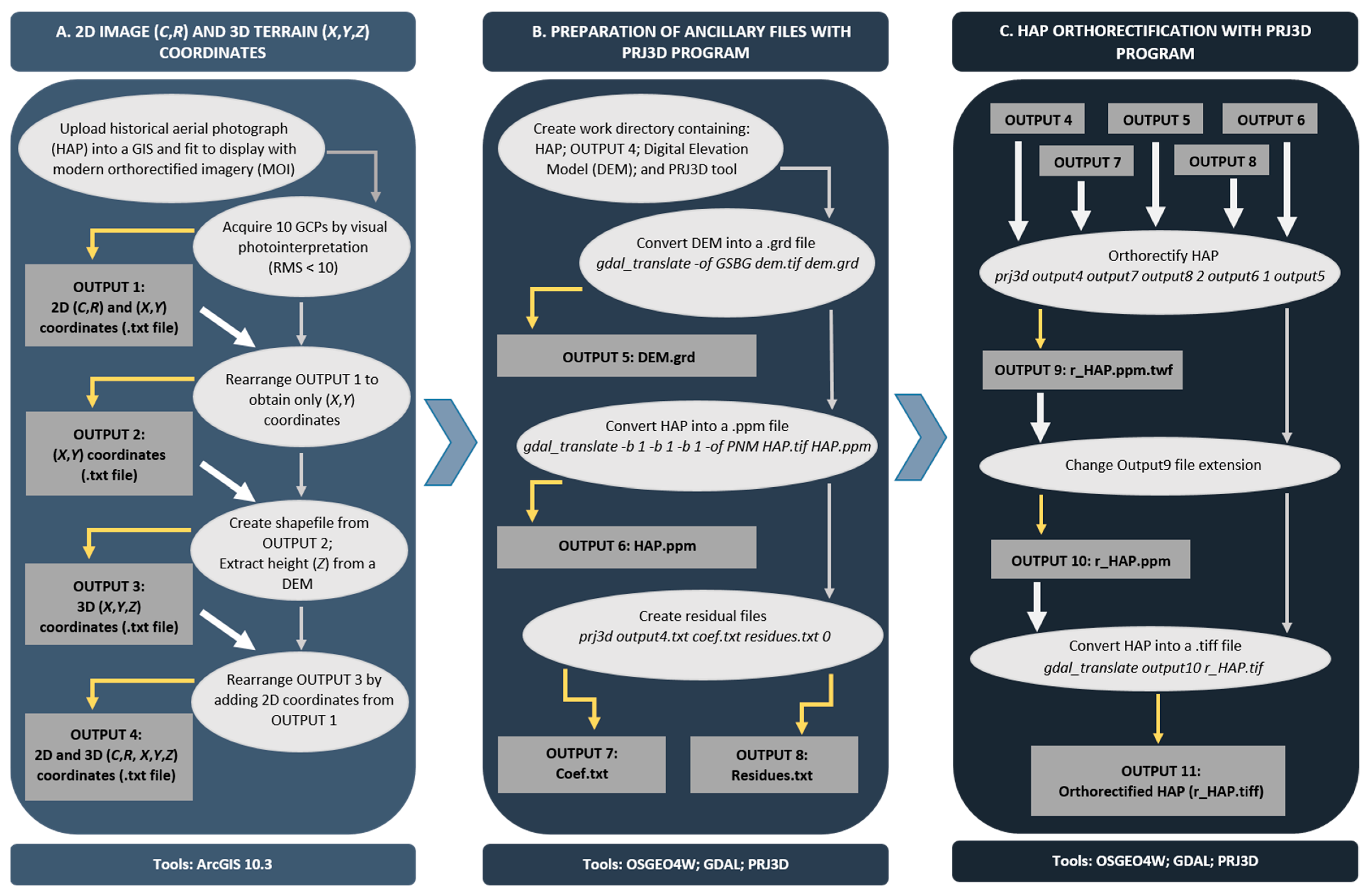
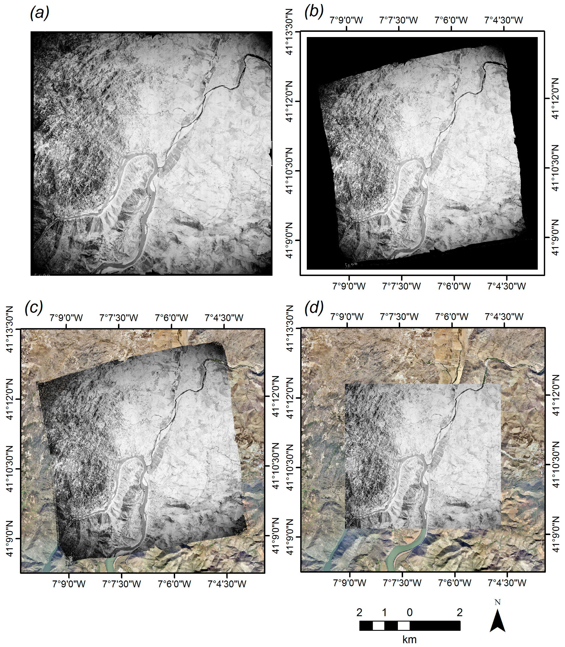
3.1. Orthorectification: The HAPO Workflow

Although in a future step, the HAPO workflow may be integrated in a GIS software (an ArcGIS toolbox or a QGIS plugin), for the time being, it was implemented as C programming language program (called “Projective 3D”—PRJ3D) and compiled with the Microsoft Visual Studio 2017 C compiler. The executable runs in the MS Windows command line, version 10 and older, taking several input files, and performs an independent orientation of individual photos using a direct linear transformation (DLT) [42] approach. The DLT method does not require camera information [16,18] but requires a point-based registration method to determine the exterior orientation by the collinearity model [17].

The DLT model is expressed by the following equations [42]:

$$\begin{gathered} C=\frac{a_{1}X+a_{2}X+a_{3}Z+a_4}{a_{9}X+a_{10}Y+a_{11}Z+1}, \\ R=\frac{a_{5}X+a_{6}X+a_{7}Z+a_8}{a_{9}X+a_{10}Y+a_{11}Z+1}, \end{gathered}$$

(1)

where (C,R) are the column and row coordinates of a point in the image matrix, in pixel units; (X,Y,Z) are the terrain coordinates (easting, northing and height) of the point in some cartographic reference system; and $\left(a_1, a_2, \dots ,a_{11}\right)$ are the coefficients characteristic of the image. These coefficients mix the exterior orientation parameters, as well as camera parameters, and can be determined if appropriate ground control points (GCPS) are available. In fact, in order to extract high-quality data from archival aerial photography, where there may be only a small number of images available and the redundancy may be low, orthorectification should be based on a reliable high-quality network of ground control information [15,16,17] well distributed in the block, especially when camera calibration information is unavailable [43]. The PRJ3D tool deals with the geometric aspects of the image orientation, to read image and terrain coordinates collected for a given photo, and to apply the least squares method to solve for the 11 unknown coefficients. For a given GCP, all coordinates will be available, so we can write 2 equations with the 11 unknown coefficients. A minimum of 6 noncollinear points would be needed to determine all the coefficients, by solving a system of equations. However, to obtain a more accurate solution, while controlling for errors, it is recommended to use more points and least-squares adjustment in parameter estimation. By providing residual errors, it is also possible to have a quality control of the process.

The least-squares adjustment produces residuals in image coordinates for each point, $\left(r_C,r_R\right)$, for which the norm is calculated: $\sqrt{r_C^2+r_R^2}.$ The program calculates the maximum of these values and the root mean square error, RMSE, in the form:

$$RMSE=\sqrt{\frac{\sum \left(r_c^2+r_R^2\right)}{n}}$$

(2)

where $n$ is the number of points used. The RMSE and the maximum norm are used to assess the quality of the process. A residual of a few pixels can be accepted, considering the accuracy of GCP coordinates as well as the acceptable accuracy, according to some predefined map scale.

The HAPO workflow for HAP orthorectification with the new “Projective 3D” (PRJ3D) program is outlined in Figure 1 and comprises three major steps: (A) acquisition of 2D and 3D coordinates; (B) preparation of ancillary files; and (C) orthorectification processing. In step A, modern orthorectified imagery (MOI) is used to help with orienting raw HAP with our HAPO workflow, namely by establishing the terrain coordinates (X,Y) for GCP’s acquisition (Equation (1)) and, later on, to check the planimetric accuracy of HAP orthomosaic. In a first approach, aerial photos are approximately georeferenced in ArcGIS, using a projective transformation, without any orthorectification, which is generally deemed acceptable in flat areas. In areas with significant relief, this procedure yields poor accuracy, often with discrepancies of 100 m, when compared to other precise geographic information. Nonetheless, this approximation facilitates the identification of common ground points when overlaid on modern orthoimages. After loading each HAP into ArcGis and fitted to display with MOI, at least 10 common points (GCPs) between HAP and MOI should be identified. The 2D coordinates (column C, row R) are provided by historical imagery, and 3D coordinates are given by MOI (easting X, northing Y) and a digital elevation model (DEM; height Z) (Output 1, Output 2, and Output 3). Image and terrain coordinates information (C, R, X, Y, Z) is then rearranged into the Coordinates.txt file, which corresponds to Output 4 of Step A.

From this point on (Steps B and C), the PRJ3D program and the obtained output data are run by the open source geospatial software OSGeo4W Shell (http://osgeo4w.osgeo.org) and the Geospatial Data Abstraction Library (GDAL) (http://www.gdal.org/) [44]. GDAL is a computer software library for reading and writing raster and vector geospatial data formats, which is released under the permissive X/MIT style free software license by the Open Source Geospatial Foundation. As a library, it presents a single abstract data model to the calling application for all supported formats. It may also be built with a variety of useful command line interface utilities for data translation and processing [44].

PRJ3D also reads a DEM of the area and projects points from ground coordinates, with elevation obtained from the DEM, onto the image space, using Equation (1). Using GDAL command lines as shown in Figure 2, the DEM and each HAP are prepared to comply with the formats required by our PRJ3D software (generating Output 5 and Output 6 of Step B), and Output 4 is run by PRJ3D in order to create residual files (Output 7 and Output 8 of Step B) for quality control. In this way, all the necessary ancillary files are obtained to proceed to Step C. At this point, PRJ3D is run and Outputs 4–8 with GDAL command lines to perform HAP orthorectification. For the obtained (C,R) image coordinates, it interpolates a greyscale value from the input image, using bilinear interpolation. In this way, an orthoimage is produced, with pixel data being brought to their correct geographical position. The orthoimage is created with a resolution specified by the user, normally larger than the DEM resolution. Nevertheless, the ideal resolution for the orthoimage is the mean ground resolution of the original photo. Finally, the obtained orthorectified HAP is converted into a tiff raster file. PRj3D is available online at http://www.fc.up.pt/pessoas/jagoncal/prj3d.zip (Supplementary Materials).

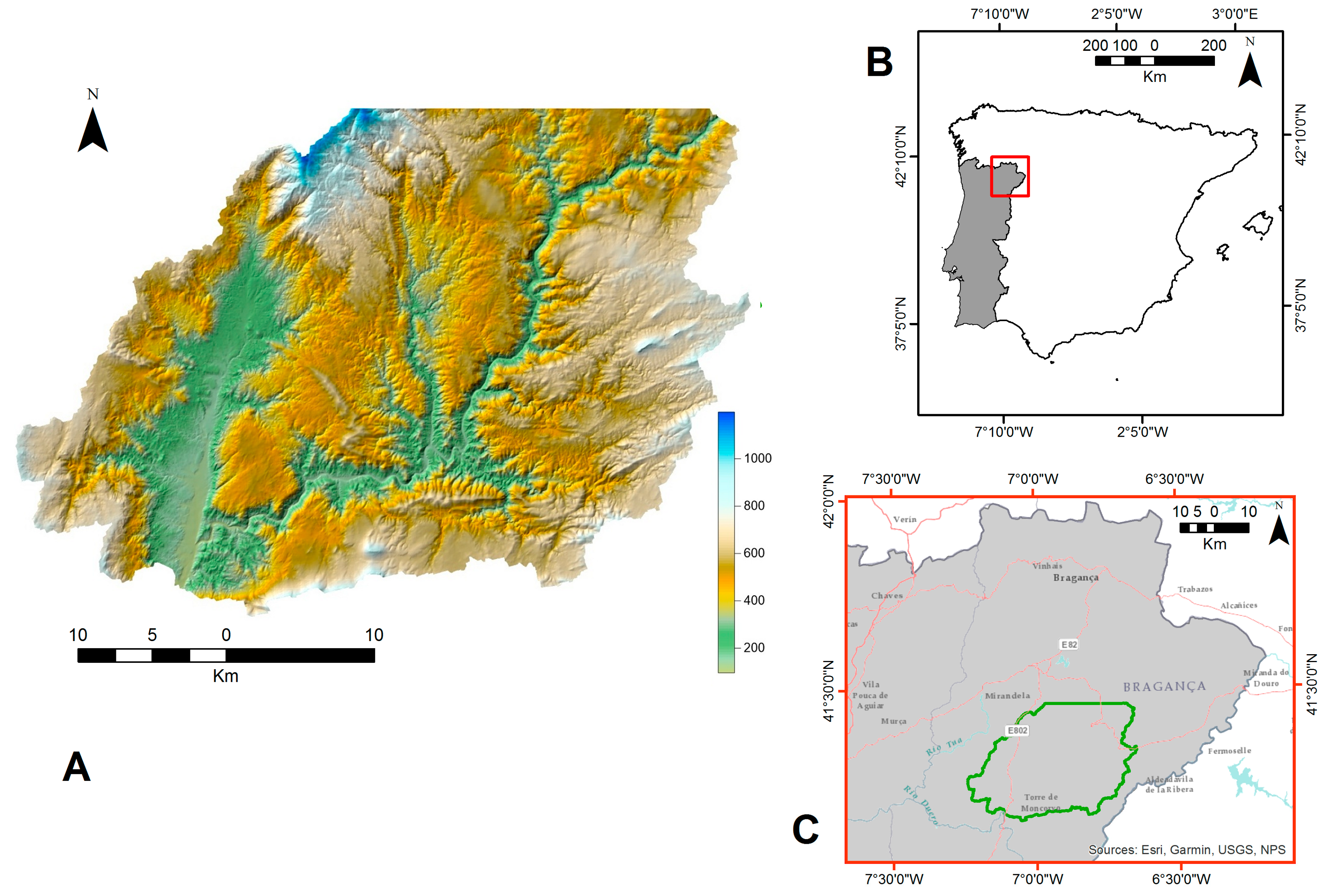
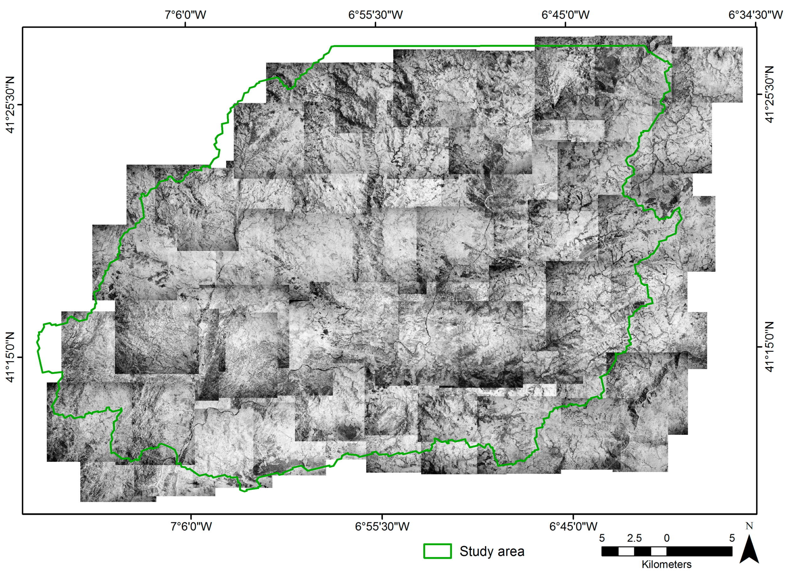
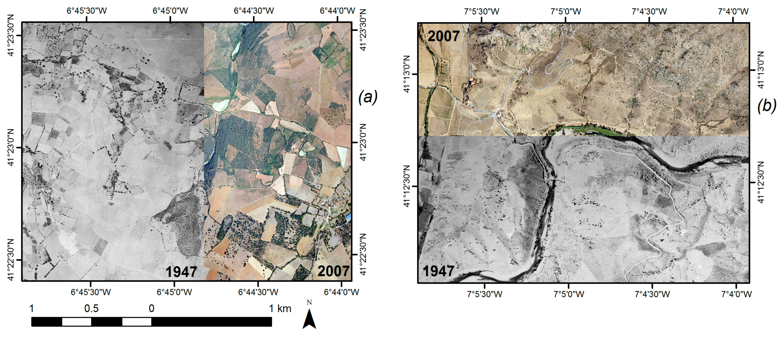
3.2. Test Area and Remote Sensing Data

The test case was conducted in a mountainous region with a Mediterranean-type climate in Northeast Portugal, covering an area of 118,636 ha and ranging in elevation from 92 m to 1199 m a.s.l. (Figure 2). The area is included in the European Union’s Natura 2000 network of nature conservation sites [45], and in the Baixo Sabor Long Term Ecological Research Site (LTER_EU_ PT_002). This area provides a valuable test case for our methodology, because it is a rugged landscape where an accurate orthorectification process is crucial to obtain detailed information on historical land cover. Furthermore, the landscape studied has suffered major land-cover changes over the years, mainly due to large scale farmland abandonment since the 1960s, thus presenting additional challenges [2,16,17,18,19,25,26], especially regarding GCPs acquisition. Finally, the availability of detailed information on land-cover dynamics was required in the scope of long-term socioecological studies carried out at this LTER site, aiming to describe and understand long-term trends in biodiversity and ecosystem services [46], which could then be used in adaptive land management strategies [8,47,48].

For our test case, we used 74 HAP of the Portuguese Army Geographic Institute (IGeoE) 1947 RAF collection covering the study area. This HAP collection derives from a systematic survey of Portugal made by the British Royal Air Force (RAF) in 1947 and is one of the largest and oldest collections of vertical aerial photos available in the archives of IGeoE in Lisbon [15]. Despite their relevance [15], they have rarely been used in ecological studies and remain relatively unexplored overall. In fact, the set of photographs used in this study had never been acquired from IGeoE in more than 65 years, nor have they ever been orthorectified.

The photos were digitalized by IGeoE in a photogrammetric scanner with a resolution of 0.021 mm [18] and presented a scale of ca. 1:29,500. There was neither a calibration certificate nor any information about the used camera, calibrated photo coordinates for fiducial marks and principal point, nor any lens distortion information. Other several classical HAP issues [26] were identified, namely: (i) a poor radiometric quality with non-uniform luminosity or image darkness; (ii) high radiometric variability within images from the same flight; (iii) a nonconstant overlap of the images; and (iv) the lack of a flight map or historical ground control points (GCPs). As the images were not stereo pairs, they presented a low and nonconstant spatial overlap and therefore were treated separately.

After loading each 1947 HAP into ArcGIS and fitting it to display with 2007 modern orthoimages provided by Portuguese Forestry Resources Institute (DGRF), we identified 10 common points per photo between 1947 images and 2007 orthophotos. To help to establish a reliable and high-quality collection of historical GCPs given the considerable land-use changes that occurred over time, we used complementary historical cartographic products at the scale of 1:500,000, including Portuguese Roads Map (1951), Diagram of the Portuguese Railways (1929) and Itinerary Map of Portugal (1937). Such historical road and railway maps often have rather unique and regionally specific characteristics, which can be useful for georeferencing HAP in regions such as Europe [3]. For each photograph, GCPs were acquired in landscape features that remained relatively unchanged and recognizable over time, such as tree fences, stone walls or roads.

The data to adjust Equation (1) included the 2D coordinates (C,R) of the GCPs identified in the 1947 historical imagery, and 3D coordinates (X,Y,Z) for the same GCPs collected from 2007 orthophotos and a digital elevation model (DEM). The DEM was generated from modern altimetry data (contours and spot heights) at a scale of 1:25,000, produced by IGeoE, with a 6 m × 6 m resolution. We then applied the HAPO workflow as described in Section 3.1. For each photograph, the root mean square error (RMSE) was calculated, as well as the maximum residual value. Their values, initially in pixel units, were converted to meters. An accuracy of 5 m (0.2 mm in a 1:25,000 reference scale) was taken as an acceptable RMSE.

In the final step, images were reformatted for mosaic building, discarding the peripheral areas, more prone to distortion problems, and focusing on the central portion of the photograph (i.e., the portion with minimum relief displacement). Since the small overlaps between adjacent photos were not regular, the area to discard was not the same for all the photos. Therefore, each photo was treated separately to obtain its maximum usable surface.

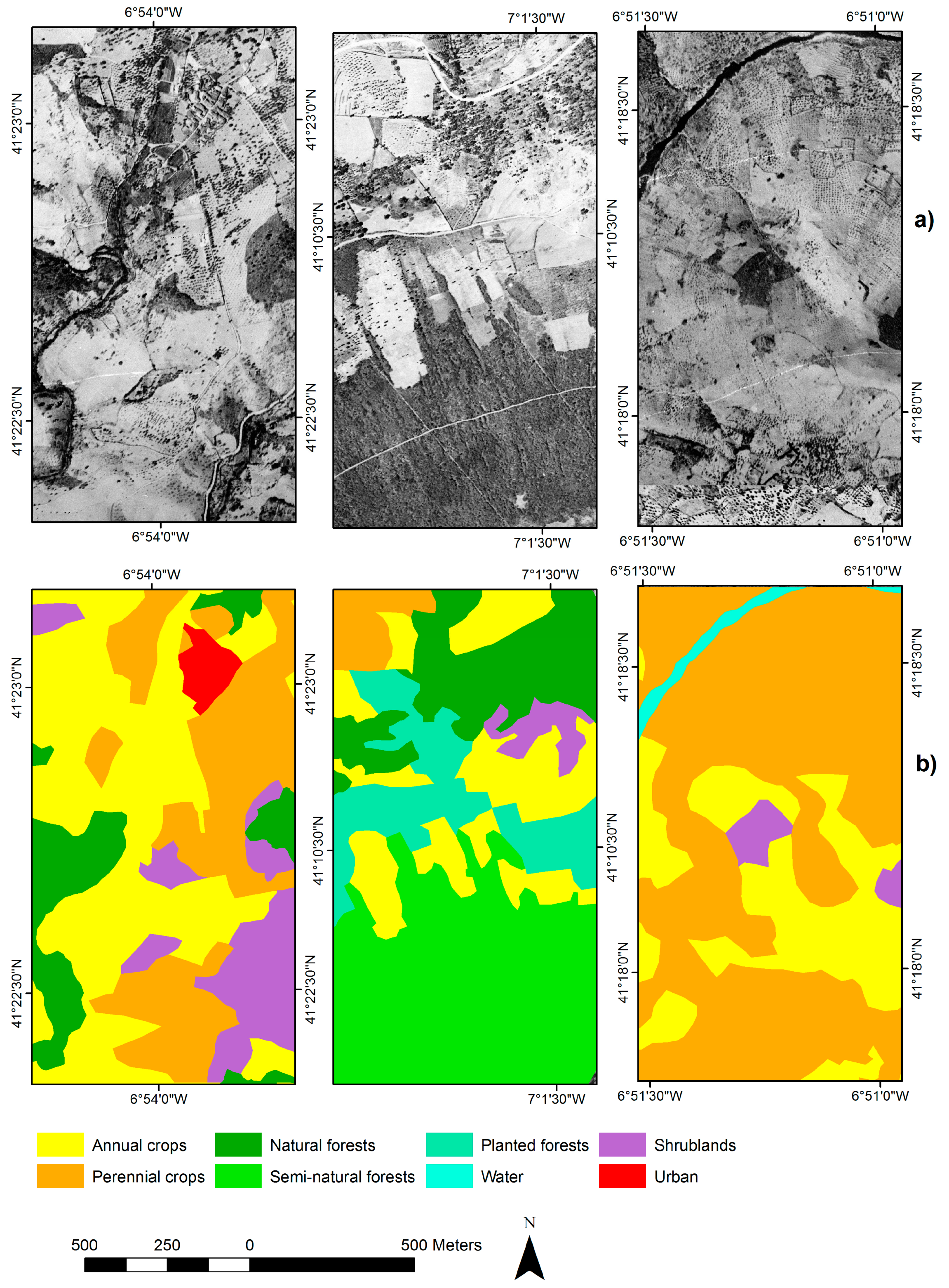
3.3. Photointerpretation and Land-Cover Mapping

After successfully being orthorectified and mosaicked, historical aerial images were subjected to visual photointerpretation to produce land-cover maps for test areas. Specifically, we produced a regular tessellation of the study area with 2 km² hexagon units, which was considered a sampling unit of sufficient size to capture spatial variations in landscape composition and heterogeneity [49,50]. A total of 56 test areas (≈10% of the study area) were then selected through a stratified random sampling approach [51], with strata corresponding to municipalities.

The procedure was based on visual interpretation, because although time-consuming, it provides reliable results [19], with trained aerial interpreters being able to successfully identify a range of different land-cover types [2,3,8,52]. Automatic or semiautomatic techniques were not used, because the radiometric quality of our historical images was not satisfactory for such approaches [19,21]. Furthermore, when a single panchromatic image is available (such as a gray-scale image obtained by HAP digitizing), an automatic image classification, in a similar way to what is done with multispectral images, is simply not possible [53].

Visual photointerpretation was made with the support of ancillary geospatial data, such as DEM, topographic maps, and other orthophotos of the same area [5,54]. We also used complementary historical data [3], such as Census data [55,56], as well as official agrarian statistical and technical reports [57,58,59,60], to improve the interpretation of landscape features. These records contained demographic as well as natural resource and agricultural information, which helped to evaluate the dominant land cover/land uses in the landscape at the time. Additionally, a site survey was carried out to check small arboreal patches that could be identified in 1947 photos. The rules of photointerpretation followed as closely as possible those used on the latest official land-cover map of Portugal (COS2007) [61], to make the data comparable across time periods.

Land-cover patches and classes were interpreted at a 1:4000 scale and hand-digitized using ArcGIS 10.3 [62]. The minimum mapping unit (MMU) was 1 hectare according to the criteria used in COS2007. Using Conefor Sensinode 2.2 [63], polygons (of one same class) under 1 hectare within 60 m from each other were grouped into multipolygon features until they complied to the MMU, assuring that (i) fine-scale information was successfully acquired and maintained in the analysis and (ii) comparability of multitemporal data sets was ensured.

The accuracy of the land-cover photointerpretation using 1947 photos could not be established quantitatively, because there were no historic reference data, and subsequent land-cover changes rendered field validation impossible [2]. Although field visits allowed the detection of some arboreal patches identified in 1947 photos, others had disappeared or changed considerably and so could not be used to validate historical land-cover mapping. To minimize these problems and thus enhance mapping accuracy, particular care was taken to cross-check photointerpretation with other sources of information, such as census data [55,56] and the official agrarian statistical and technical reports [57,58,59,60].

4. Results

4.1. Historical Orthophotographs and Orthomosaic

Application of the HAPO methodology successfully processed all images (Figure 3), producing an orthomosaic of 74 orthorectified HAP for our test area (Figure 4). Visual inspection of the orthorectified images overlaid on modern 2007 orthomaps and road networks indicated a good matching between old and recent geographic information (Figure 5). This was confirmed by the low average value and standard deviation of RMSE (1.97 m and 1.00 m, respectively), which ranged between aerial photographs from 0.90 m to 5.88 m. Only one out of 74 images processed had an RMSE above 5 m (Figure 6), which was taken as the reference value for acceptable accuracy. The maximum errors were slightly higher, still with only 2 values above 10 m. Overall, images covering areas with steeper slopes and with more pronounced landscape changes over the years had the highest RMSE values. Nevertheless, the accuracy obtained was well within that acceptable for the reference map scale of 1:25,000.

4.2. Land-Cover Mapping

Our historical aerial photographs (Figure 6a) allowed the identification of eight different land-cover classes in the landscapes of 1947: annual crops (covering 61.24% of the total photointerpreted area), perennial crops (14.21%), shrublands (11.77%), natural forests (7.88%), seminatural forests (1.33%), planted forests (3%), water (0.28%), and urban (0.28%) (Figure 6b). It was possible to confidently identify and delineate small to medium-sized and large patches, ranging from 0.1 to 200 ha, allowing a detailed socioecological description of the 1947 landscape in our test area, despite the marked landscape change that occurred over time.

5. Discussion

Our study described and provided a successful application of the new HAPO workflow to orthorectify historical aerial photographs (HAP). The local case study developed in Portugal contained many of the problems commonly faced by researchers wanting to use HAP and showed that HAPO can produce spatial information with the accuracy required to describe and understand long-term socioecological patterns and processes. We showed that HAPO can deal with non-overlapping or marginally overlapping HAP sets, lack of a flight map, difficulties to identify ground control points (GCPs) in changing landscapes, poor radiometric quality, and high radiometric variability between images, among other factors. Despite these problems, the final orthoimages had high geometric accuracy and could be used to produce land-cover maps that will later feed into studies addressing questions related to long term socioecological dynamics. Therefore, we believe that HAPO can be used by a wide range of researchers dealing with similar problems elsewhere, representing a significant advance to harness the power of historical information available in HAP.

Through the application of HAPO to our particular test case, it was clear that achieving high accuracy in HAP orthorectification and georeferencing requires that care should be taken with a number of critical aspects. First, a good resolution digital elevation model is required to achieve the best results, particularly in rugged landscapes such as ours, where significant changes in elevation over small areas represent a challenge for the correct application of our procedure. Second, it is important to have access to modern orthorectified and georeferenced imagery, or other adequate cartographic information, without which it may be nearly impossible to obtain accurate GCPs. Third, GCPs should be well distributed along the historical image and preferentially not placed near the borders to avoid highest correspondence errors between HAP and modern orthoimages. Fourth, when covering highly rugged areas, steep slopes and landscapes suffering pronounced changes over the years, it is recommended to acquire a larger number of GCPs to help to reduce positional errors. Finally, we highlight the importance of using complementary cartographic products such as historical road and railway maps, as well as historical datasets such as Census data and unpublished reports contemporary to the HAP, which can be very helpful to identify GCPs in the orthorectification process and to support the visual photointerpretation to produce land-cover maps.

Overall, the new HAPO workflow presented and tested in this study represents a valuable addition to the toolkit of researchers interested in landscape ecology, socioecological patterns and dynamics, long-term ecology, and global change, by offering the possibility to capture the unique and extremely valuable historic memory of our landscapes, and permitting a detailed and objective look-back in time [21]. Reconstructing and recovering historical patterns and processes is key to understanding how present conditions came about, with the analysis of landscape change drivers providing an essential basis [64] not only for monitoring landscape diversity [57,58] and for investigating changes in vegetation and landscape structure [35,36,37], but also to understand human–environment interactions and how they have shaped contemporary landscapes [64,65]. This unique information can be used by managers and researchers for a great variety of environmental studies and applications [1,2] and can definitely contribute to more informed policy, management, and restoration decisions [48,64,65,66,67,68,69].

Future work may consider the adaptation of the program to the Python programming language in order to include it as an additional GIS command, for example, in the form of a QGIS plugin. This will make it more friendly for nonspecialist GIS users.

References

1. Morgan, J.L.; Gergel, S.E. Quantifying historic landscape heterogeneity from aerial photographs using object-based analysis. Landsc. Ecol. 2010, 25, 985–998. [Google Scholar] [CrossRef]
2. Morgan, J.L.; Gergel, S.E.; Coops, N.C. Aerial Photography: A Rapidly Evolving Tool for Ecological Management. Bioscience 2010, 60, 47–59. [Google Scholar] [CrossRef]
3. Tomscha, S.A.; Sutherland, I.J.; Renard, D.; Gergel, S.E.; Rhemtulla, J.M.; Bennett, E.M.; Daniels, L.D.; Eddy, I.M.S.; Clark, E.E. A guide to historical data sets for reconstructing ecosystem service change over time. Bioscience 2016, 66, 747–762. [Google Scholar] [CrossRef]
4. Swetnam, R.D.; Fisher, B.; Mbilinyi, B.P.; Munishi, P.K.T.; Willcock, S.; Ricketts, T.; Mwakalila, S.; Balmford, A.; Burgess, N.D.; Marshall, A.R.; et al. Mapping socio-economic scenarios of land cover change: A GIS method to enable ecosystem service modelling. J. Environ. Manag. 2011, 92, 563–574. [Google Scholar] [CrossRef] [PubMed]
5. Pelorosso, R.; Della Chiesa, S.; Tappeiner, U.; Leone, A.; Rocchini, D. Stability analysis for defining management strategies in abandoned mountain landscapes of the Mediterranean basin. Landsc. Urban Plan. 2011, 103, 335–346. [Google Scholar] [CrossRef]
6. Gennaretti, F.; Ripa, M.N.; Gobattoni, F.; Boccia, L.; Pelorosso, R. A methodology proposal for land cover change analysis using historical aerial photos. Geogr. Reg. Plan. 2011, 4, 542–556. [Google Scholar]
7. Dittrich, A.; von Wehrden, H.; Abson, D.J.; Bartkowski, B.; Cord, A.F.; Fust, P.; Hoyer, C.; Kambach, S.; Meyer, M.A.; Radzevičiūtė, R.; et al. Mapping and analysing historical indicators of ecosystem services in Germany. Ecol. Indic. 2017, 75, 101–110. [Google Scholar] [CrossRef]
8. Tomscha, S.A.; Gergel, S.E. Ecosystem Service Trade-offs and Synergies. Ecol. Soc. 2015, 21, 43. [Google Scholar] [CrossRef]
9. Vogels, M.F.A.; de Jong, S.M.; Sterk, G.; Addink, E.A. Agricultural cropland mapping using black-and-white aerial photography, Object-Based Image Analysis and Random Forests. Int. J. Appl. Earth Obs. Geoinf. 2017, 54, 114–123. [Google Scholar] [CrossRef]
10. Jiang, M.; Bullock, J.M.; Hooftman, D.A.P. Mapping ecosystem service and biodiversity changes over 70 years in a rural English county. J. Appl. Ecol. 2013, 50, 841–850. [Google Scholar] [CrossRef] [Green Version]
11. Cousins, S.A.O.; Auffret, A.G.; Lindgren, J.; Tränk, L. Regional-scale land-cover change during the 20th century and its consequences for biodiversity. Ambio 2015, 44, 17–27. [Google Scholar] [CrossRef] [PubMed] [Green Version]
12. Willcock, S.; Phillips, O.L.; Platts, P.J.; Swetnam, R.D.; Balmford, A.; Burgess, N.D.; Ahrends, A.; Bayliss, J.; Doggart, N.; Doody, K.; et al. Land cover change and carbon emissions over 100 years in an African biodiversity hotspot. Glob. Chang. Biol. 2016, 22, 2787–2800. [Google Scholar] [CrossRef] [PubMed] [Green Version]
13. Belward, A.S.; Skøien, J.O. Who launched what, when and why; trends in global land-cover observation capacity from civilian earth observation satellites. ISPRS J. Photogramm. Remote Sens. 2015, 103, 115–128. [Google Scholar] [CrossRef]
14. Giordano, S.; Le Bris, A.; Mallet, C. Fully Automatic Analysis of Archival Aerial Images Current status and challenges. In Proceedings of the 2017 Joint Urban Remote Sensing Event (JURSE), Dubai, UAE, 6–8 March 2017; pp. 1–4. [Google Scholar]
15. Redweik, P.; Roque, D.; Marques, A.; Matildes, R.; Marques, F. Recovering Portugal Aerial Images Repository. ISPRS High-Resolut. Earth Imaging Geospat. Inf. 2009, 38, 1–4. [Google Scholar]
16. Ma, R.; Buchwald, A. Orthorectify Historical Aerial Photographs Using DLT. In Proceedings of the ASPRS 2012 Annual Conference, Sacramento, CA, USA, 19–23 March 2012. [Google Scholar]
17. Nagarajan, S.; Schenk, T. Feature-based registration of historical aerial images by Area Minimization. ISPRS J. Photogramm. Remote Sens. 2016, 116, 15–23. [Google Scholar] [CrossRef]
18. Gonçalves, J.A. Automatic orientation and mosaicking of archived aerial photography using structure from motion. Int. Arch. Photogramm. Remote Sens. Spat. Inf. Sci. 2016, 40, 123–126. [Google Scholar] [CrossRef]
19. Nocerino, E.; Menna, F.; Remondino, F. Multi-Temporal Analysis of Landscapes and Urban Areas. Int. Arch. Photogramm. Remote Sens. Spat. Inf. Sci. 2012, 39-B4, 85–90. [Google Scholar] [CrossRef]
20. Stoate, C.; Báldi, A.; Beja, P.; Boatman, N.D.; Herzon, I.; van Doorn, A.; de Snoo, G.R.; Rakosy, L.; Ramwell, C. Ecological impacts of early 21st century agricultural change in Europe—A review. J. Environ. Manag. 2009, 91, 22–46. [Google Scholar] [CrossRef]
21. Nebiker, S.; Lack, N.; Deuber, M. Building change detection from historical aerial photographs using dense image matching and object-based image analysis. Remote Sens. 2014, 6, 8310–8336. [Google Scholar] [CrossRef]
22. Du, S.; Zhang, Y.; Qin, R.; Yang, Z.; Zou, Z.; Tang, Y.; Fan, C. Building Change Detection Using Old Aerial Images and New LiDAR Data. Remote Sens. 2016, 8, 1030. [Google Scholar] [CrossRef]
23. Cardenal, J.; Delgado, J.; Mata, E.; González, A.; Olague, I. Use of Historical Flight for Landslide Monitoring. In Proceedings of the 7th International Symposium on Spatial Accuracy Assessment in Natural Resources and Environmental Sciences, Lisbon, Portugal, 5–7 July 2006; pp. 129–138. [Google Scholar]
24. Luman, D.E.; Stohr, C.J.; Hunt, L. Digital reproduction of historical aerial photographic prints for preserving a deteriorating archive. Photogramm. Eng. Remote Sens. 1997, 63, 1171–1179. [Google Scholar]
25. Ma, R. Rational Function Model in Processing Historical Aerial Photographs. Photogramm. Eng. Remote Sens. 2013, 79, 337–345. [Google Scholar] [CrossRef]
26. Redecker, A.P. Redecker. In Historical Aerial Photographs and Digital Photogrammetry for Impact Analyses on Derelict Land Sites in Human Settlement Areas; IAPRS&SIS: Beijing, China, 2008; pp. 5–10. [Google Scholar]
27. Véga, C.; St-Onge, B. Height growth reconstruction of a boreal forest canopy over a period of 58 years using a combination of photogrammetric and lidar models. Remote Sens. Environ. 2008, 112, 1784–1794. [Google Scholar] [CrossRef] [Green Version]
28. Prokešová, R.; Kardoš, M.; Medveďová, A. Landslide dynamics from high-resolution aerial photographs: A case study from the Western Carpathians, Slovakia. Geomorphology 2010, 115, 90–101. [Google Scholar] [CrossRef]
29. De Agar, P.M.; Ortega, M.; de Pablo, C.L. A procedure of landscape services assessment based on mosaics of patches and boundaries. J. Environ. Manag. 2016, 180, 214–227. [Google Scholar] [CrossRef]
30. Rapinel, S.; Clément, B.; Dufour, S.; Hubert-Moy, L. Fine-Scale Monitoring of Long-term Wetland Loss Using LiDAR Data and Historical Aerial Photographs: The Example of the Couesnon Floodplain, France. Wetlands 2018, 38, 423–435. [Google Scholar] [CrossRef]
31. Bastian, O.; Grunewald, K.; Syrbe, R.U.; Walz, U.; Wende, W. Landscape services: The concept and its practical relevance. Landsc. Ecol. 2014, 29, 1463–1479. [Google Scholar] [CrossRef]
32. McCluskey, E.M.; Matthews, S.N.; Ligocki, I.Y.; Holding, M.L.; Lipps, G.J.; Hetherington, T.E. The importance of historical land use in the maintenance of early successional habitat for a threatened rattlesnake. Glob. Ecol. Conserv. 2018, 13, e00370. [Google Scholar] [CrossRef]
33. Wang, H.; Ellis, E.C. Spatial accuracy of orthorectified IKONOS imagery and historical aerial photographs across five sites in China. Int. J. Remote Sens. 2005, 26, 1893–1911. [Google Scholar] [CrossRef]
34. Nyssen, J.; Petrie, G.; Mohamed, S.; Gebremeskel, G.; Seghers, V.; Debever, M.; Hadgu, K.M.; Stal, C.; Billi, P.; Demaeyer, P.; et al. Recovery of the aerial photographs of Ethiopia in the 1930s. J. Cult. Herit. 2016, 17, 170–178. [Google Scholar] [CrossRef] [Green Version]
35. Lydersen, J.M.; Collins, B.M. Change in Vegetation Patterns Over a Large Forested Landscape Based on Historical and Contemporary Aerial Photography. Ecosystems 2018, 21, 1348–1363. [Google Scholar] [CrossRef]
36. Rocchini, D.; Perry, G.L.W.; Salerno, M.; Maccherini, S.; Chiarucci, A. Landscape change and the dynamics of open formations in a natural reserve. Landsc. Urban Plan. 2006, 77, 167–177. [Google Scholar] [CrossRef]
37. Aguiar, F.C.; Martins, M.J.; Silva, P.C.; Fernandes, M.R. Riverscapes downstream of hydropower dams: Effects of altered flows and historical land-use change. Landsc. Urban Plan. 2016, 153, 83–98. [Google Scholar] [CrossRef]
38. Beller, E.E.; Downs, P.W.; Grossinger, R.M.; Orr, B.K.; Salomon, M.N. From past patterns to future potential: Using historical ecology to inform river restoration on an intermittent California river. Landsc. Ecol. 2016, 31, 581–600. [Google Scholar] [CrossRef]
39. Lu, P.; Yang, R.; Chen, P.; Guo, Y.; Chen, F.; Masini, N.; Lasaponara, R. On the use of historical archive of aerial photographs for the discovery and interpretation of ancient hidden linear cultural relics in the alluvial plain of eastern Henan, China. J. Cult. Herit. 2017, 23, 20–27. [Google Scholar] [CrossRef]
40. Turner, M.; Gardner, R.H.; O’Neill, R. Landscape Ecology in Theory and Practice; Springer: New York, NY, USA, 2001; ISBN 0-387-95122-9. [Google Scholar]
41. Vihervaara, P.; Kumpula, T.; Tanskanen, A.; Burkhard, B. Ecosystem services-A tool for sustainable management of human-environment systems. Case study Finnish Forest Lapland. Ecol. Complex. 2010, 7, 410–420. [Google Scholar] [CrossRef]
42. Abdel-Aziz, Y.I.; Karara, H.M. Direct Linear Transformation from Comparator Coordinates into Object Space Coordinates in Close-range Photogrammetry. In Proceedings of the ASP Symposium on Close-Range Photogrammtery; American Society of Photogrammetry: Falls Church, VA, USA, 1971; pp. 1–18. [Google Scholar]
43. Aguilar, M.A.; Aguilar, F.J.; Fernandez, I.; Mills, J.P. Accuracy Assessment of Commercial Self-Calibrating Bundle Adjustment Routines Applied to Archival Aerial Photography. Photogramm. Rec. 2013, 28, 96–114. [Google Scholar] [CrossRef]
44. Contributors, GDAL/OGR Geospatial Data Abstraction Software Library. Open Source Geospatial Foundation. Available online: https://gdal.org (accessed on 30 September 2018).
45. Kati, V.; Hovardas, T.; Dieterich, M.; Ibisch, P.L.; Mihok, B.; Selva, N. The challenge of implementing the European network of protected areas Natura 2000. Conserv. Biol. 2015, 29, 260–270. [Google Scholar] [CrossRef]
46. Renard, D.; Rhemtulla, J.M.; Bennett, E.M. Historical dynamics in ecosystem service bundles. Proc. Natl. Acad. Sci. USA 2015, 112, 13411–13416. [Google Scholar] [CrossRef] [Green Version]
47. Burkhard, B.; Kroll, F.; Nedkov, S.; Müller, F. Mapping ecosystem service supply, demand and budgets. Ecol. Indic. 2012, 21, 17–29. [Google Scholar] [CrossRef]
48. Morán-Ordóñez, A.; Bugter, R.; Suárez-Seoane, S.; de Luis, E.; Calvo, L. Temporal Changes in Socio-Ecological Systems and Their Impact on Ecosystem Services at Different Governance Scales: A Case Study of Heathlands. Ecosystems 2013, 16, 765–782. [Google Scholar] [CrossRef]
49. White, D.; Preston, E.M.; Freemark, K.E.; Kiester, A.R. Landscape Ecological Analysis. In Landscape Ecological Analysis: Issues and Applications; Klopatek, J.M., Gardner, R.H., Eds.; Springer: New York, NY, USA, 1999; pp. 127–152. ISBN 978-1-4612-6804-8. [Google Scholar]
50. Birch, C.P.D.; Oom, S.P.; Beecham, J.A. Rectangular and hexagonal grids used for observation, experiment and simulation in ecology. Ecol. Model. 2007, 206, 347–359. [Google Scholar] [CrossRef]
51. De Gruijter, J.; Brus, D.J.; Bierkens, M.F.; Knotters, M. Sampling for Natural Resource Monitoring; Springer: Berlin/Heidelberg, Germany, 2006. [Google Scholar]
52. Berg, Å.; Wretenberg, J.; Zmihorski, M.; Hiron, M.; Pärt, T. Linking occurrence and changes in local abundance of farmland bird species to landscape composition and land-use changes. Agric. Ecosyst. Environ. 2015, 204, 1–7. [Google Scholar] [CrossRef] [Green Version]
53. Caridade, C.M.R.; Marçal, A.R.S.; Mendonça, T. The use of texture for image classification of black & white air photographs. Int. J. Remote Sens. 2008, 29, 593–607. [Google Scholar] [CrossRef]
54. Pelorosso, R.; Leone, A.; Boccia, L. Land cover and land use change in the Italian central Apennines: A comparison of assessment methods. Appl. Geogr. 2009, 29, 35–48. [Google Scholar] [CrossRef]
55. Instituto Nacional de Estatística (Statistics Portugal). XIX Recenseamento Geral da População for 1950 (Population Census); Instituto Nacional de Estatística (Statistics Portugal): Lisbon, Portugal, 1952.
56. Instituto Nacional de Estatística (Statistics Portugal). VII Recenseamento Geral da População for 1940 (Population Census); Instituto Nacional de Estatística (Statistics Portugal): Lisbon, Portugal, 1946.
57. Instituto Nacional de Estatística (Statistics Portugal). Estatísticas Agrícolas (Agrarian Statistics); Instituto Nacional de Estatística (Statistics Portugal): Lisbon, Portugal, 1947.
58. Instituto Nacional de Estatística (Statistics Portugal). O Problema do Trigo. Folheto n. 50, Separata n. 3 do Centro de Estudos Económicos; Instituto Nacional de Estatística (Statistics Portugal): Lisbon, Portugal, 1946.
59. Instituto Nacional de Estatística (Statistics Portugal). Portugal: 1935–1985; Instituto Nacional de Estatística (Statistics Portugal): Lisbon, Portugal, 1985.
60. Ministério da Agricultura. Campanha do Trigo, 1929–1930, Folheto no 1; Ministério da Agricultura: Lisbon, Portugal, 1930.
61. DGT. Available online: http://www.dgterritorio.pt/ cartografia_e_geodesia/cartografia/cartografia_tematica/carta_de_ocupacao_do_solo__cos_/cos__2007/ (accessed on 16 November 2018).
62. ESRI ArcGIS Desktop. Release 10.3; Environmental Systems Research Institute: Redlands, CA, USA, 2014. [Google Scholar]
63. Saura, S.; Torné, J. Conefor Sensinode 2.2: A software package for quantifying the importance of habitat patches for landscape connectivity. Environ. Model. Softw. 2009, 24, 135–139. [Google Scholar] [CrossRef]
64. Haase, D.; Walz, U.; Neubert, M.; Rosenberg, M. Changes to Central European landscapes-Analysing historical maps to approach current environmental issues, examples from Saxony, Central Germany. Land Use Policy 2007, 24, 248–263. [Google Scholar] [CrossRef]
65. Yeh, C.T.; Huang, S.L. Investigating spatiotemporal patterns of landscape diversity in response to urbanization. Landsc. Urban Plan. 2009, 93, 151–162. [Google Scholar] [CrossRef]
66. Leyk, S.; Boesch, R.; Weibel, R. Saliency and semantic processing: Extracting forest cover from historical topographic maps. Pattern Recognit. 2006, 39, 953–968. [Google Scholar] [CrossRef]
67. Tortora, A.; Statuto, D.; Picuno, P. Rural landscape planning through spatial modelling and image processing of historical maps. Land Use Policy 2015, 42, 71–82. [Google Scholar] [CrossRef]
68. Armstrong, C.G.; Shoemaker, A.C.; McKechnie, I.; Ekblom, A.; Szabó, P.; Lane, P.J.; McAlvay, A.C.; Boles, O.J.; Walshaw, S.; Petek, N.; et al. Anthropological contributions to historical ecology: 50 questions, infinite prospects. PLoS ONE 2017, 12, e0171883. [Google Scholar] [CrossRef]
69. Rhemtulla, J.M.; Mladenoff, D.J. Why history matters in landscape ecology. Landsc. Ecol. 2007, 22, 1–3. [Google Scholar] [CrossRef]
Figure 1. Historical aerial photographs orthorectification (HAPO) general workflow. PRJ3D stands for our new program “Projective 3D”. Round shapes describe tasks (Geospatial Data Abstraction Library (GDAL) command lines are shown in italics) and the outputs are shown in grey boxes. Light grey arrows indicate tasks sequence; yellow arrows indicate outputs generated by tasks; and white arrows indicate data input required for each task.
Remotesensing 11 01388 g001
Figure 2. Digital elevation model for the test area (A) and its location in the Iberian Peninsula (B) and in Northeast Portugal (C).
Remotesensing 11 01388 g002
Figure 3. Examples of input and output historical aerial photographs: (a) original HAP; (b) orthorectified HAP (c,d) orthorectified HAP overlaid with georeferenced contemporary image (Portuguese Forestry Resources Institute (DGRF) 2007); and (d) orthorectified HAP central portion for mosaic building.
Remotesensing 11 01388 g003
Figure 4. Orthomosaic of the 74 orthorectified historical aerial photographs of 1947, produced with the HAPO workflow.
Remotesensing 11 01388 g004
Figure 5. Orthorectified and georeferenced 1947 historical aerial photographs overlaid with two 2007 georeferenced orthophotos (a,b).
Remotesensing 11 01388 g005
Figure 6. Selected portions of orthorectified 1947 historical aerial photographs (a); and corresponding 1947 land-cover classification (b).
Remotesensing 11 01388 g006