The Integration of Photodiode and Camera for Visible Light Positioning by Using Fixed-Lag Ensemble Kalman Smoother

Abstract

Visible Light Positioning (VLP) has become one of the most popular positioning and navigation systems in this decade. Filter-based VLP systems can provide real-time solutions but have limited accuracy. On the contrary, fixed-interval smoothers can help VLP achieve higher accuracy but require post-processing. In this article, a trade-off solution, Fixed-Lag Ensemble Kalman Smoother (FLEnKS), is proposed for VLP to achieve a semi-real-time and accurate positioning solution. The forward part of the FLEnKS is based on the Ensemble Kalman Filter (EnKF), which uses stochastic sampling with ensemble members and enables a better reflection of the features of nonlinear systems. The backward filter in the FLEnKS compensates for the estimation error from the forward filter using the linearization based on error states and further reduces the estimation error. Furthermore, multiple data from both photodiode (PD) and camera are fused in the proposed FLEnKS for VLP, which further improves the accuracy of conventional VLP with a single data source. Preliminary field test results show that the proposed FLEnKS provides a semi-real-time positioning solution with the average 3D positioning accuracy of 15.63 cm in dynamic tests.

1. Introduction

Visible Light Positioning (VLP) is becoming increasingly popular for indoor positioning and navigation because of its high accuracy and the extensive usage of Light Emitting Diodes (LEDs) [1]. Filters such as Kalman Filter (KF) and Particle Filter (PF) are widely employed in VLP systems to improve the real-time positioning accuracy [2]. Since filters only use current and previous information [3,4,5,6,7], it is worthwhile to use other techniques such as smoothing to further improve the localization accuracy and robustness. ‘Localization’ mentioned in this article refers to locating a receiver.

Smoothing algorithms can use previous, current, and future information for localization, which improves the positioning accuracy but introduces latency. Smoothing is commonly used instead of real-time localization for post-mission applications. To the best of the authors’ knowledge, the smoothing technique has not been used in the VLP except our previous work [8]. It is challenging to propose a smoother to improve positioning accuracy with acceptable latency. For VLP applications, the smoother should have the following capabilities: (a) real/semi-real time; (b) high-accuracy localization; and (c) possible application to non-linear systems.

The existing smoothers can be classified into three groups: fixed-interval smoother, fixed-point smoother, and fixed-lag smoother [9]. The fixed-interval smoother requires the estimates of entire data samples and can only be used offline [8]. The fixed-tablepoint smoother is often used to calibrate the estimation results of a certain point. The fixed-lag smoother uses a sliding window to smooth the estimation results of several previous points, which can provide a semi-real-time solution. Thus, the fixed-lag smoother is more appropriate for real/semi-real time positioning, localization, and tracking applications.

A Fixed-Lag Kalman Smoother (FLKS) is proposed in [10] for the sequential estimation of atmospheric carbon dioxide fluxes. The FLKS steps through an inversion in multiple steps, and the covariance information between sequential sets of fluxes is saved. However, FLKS is based on KF and only can be employed for a linear problem, which is not appropriate for VLP. To deal with non-linear systems, a Fixed-Lag Extended Kalman Smoother (FLEKS) is proposed in [11] based on the Extended Kalman Filter (EKF). However, EKF converts the nonlinear model into an approximate linear model through Taylor series expansion, which produces truncated errors [12].

A study [13] derives a Fixed-Lag Sigma-Point Kalman Smoother (FLSPKS) including a forward and a backward filter for indoor localization. The forward filter is a standard Sigma-Point Kalman Filter (SPKF) using the Weighted Statistical Linear Regression (WSLR) [14]. Thus, the backward filter can be formulated without inverting the nonlinear dynamics. The SPKF is a deterministic sampling algorithm with certain sample points. In the SPKF, the number of the sample points is of the same order as the dimension of the system state vector, which cannot precisely reflect the states of high-dimensional and nonlinear systems.

To reflect the system states more precisely, an article [15] proposed a fixed-lag Particle Smoother (PS). The PF used in PS applies a stochastic sampling algorithm. Similar to the PS, the Ensemble Kalman Smoother (EnKS) based on the Ensemble Kalman Filter (EnKF) also uses model trajectories called either particles or ensemble members to track the true solution of the system. The EnKF samples the points randomly with ensemble members to realize the numerical computation of the state covariance matrix, which better reflects the states of non-linear systems than the SPKF. The EnKF has been widely used in high-order and nonlinear meteorology and geology models [16] because of its high accuracy. Besides, the EnKF is an approximated version of the PF without the step involving importance weights [17], which means the EnKS is less complex than PS. Considering the accuracy and positioning latency, the fix-lag EnKS is adopted in this article.

Since the smoothing technique has not been used in VLP systems except our previous work [9], in this article, a novel fixed-lag smoother based on EnKF is proposed to achieve better positioning accuracy at the cost of acceptable positioning latency. The main contributions of this article are summarized as follows:

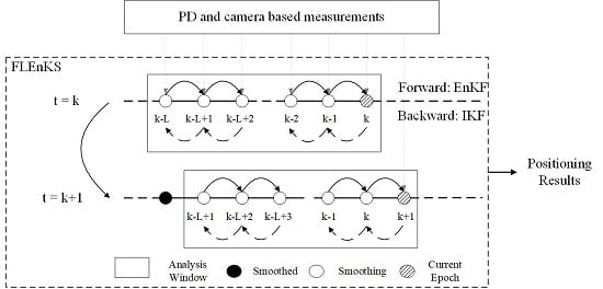
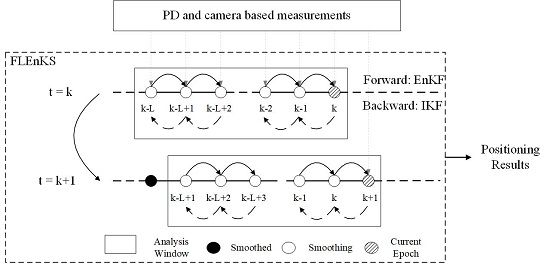
• A novel fixed-lag EnKS (FLEnKS) is proposed in this article for semi-real-time VLP. The FLEnKS uses a sliding analysis window of several points to realize semi-real-time positioning. Besides, the FLEnKS applies a two-filter structure, in which a forward EnKF with Statistical Linear Regression (SLR) and a backward modified Information Kalman Filter (IKF) with error states are performed. The backward filter compensates the estimation error of the forward filter to improve accuracy. Moreover, the proposed FLEnKS adopts SLR instead of WSLR to reduce the complexity.
• The data from both photodiode (PD) and camera are fused in the proposed FLEnKS for VLP, which further improves the accuracy of the conventional VLP with a single data source. For the purpose of comparison, other fixed-lag smoothers proposed in previous articles are also implemented in this research. Compared to the existing smoothing techniques, the proposed FLEnKS provided more accurate localization solutions, especially at corners.

The rest of this article is organized as follows. The FLEnKS algorithm is presented in Section 2. The application of FLEnKS in the VLP system is described in Section 3. The experimental results and analysis are discussed in Section 4, and the conclusions are presented in Section 5.

2. Fixed-Lag Ensemble Kalman Smoother

This section presents the algorithm of the proposed FLEnKS based on the two-filter architecture. In each analysis window of L epochs, FLEnKS includes an EnKF with SLR as the forward part and a modified IKF as the backward part, respectively. The process of the FLEnKS is shown in Figure 1. In Figure 1, the present time epoch is illustrated in black solid circles. In each analysis window with L epochs, the forward filter (i.e., the EnKF) processes the data samples sequentially, and the backward filter (i.e., the IKF) reversely processes the data samples to compensate the estimation error of the forward filter. The smoother combines the update estimation of the forward filter and the prediction estimation of the backward filter to provide a more accurate estimation. Then, the analysis window shifts by one epoch forward to the next analysis window and repeats the smoother algorithm until the final epoch. The details of the forward and backward filters and the smoother are shown in this section.

2.1. State-Space Model

The positioning problem can often be described as an estimation problem of the state of a discrete-time nonlinear dynamic system, and the nonlinear state-space model at the epoch k is often described as follows:

$$x_{k+1}=f(x_k)+{\mathsf{\omega }}_k$$

(1)

$$z_k=h(x_k)+{\mathsf{\eta }}_k$$

(2)

where $x_k\in {ℝ}^{n\times 1}$ is the state vector, $z_k\in {ℝ}^{m\times 1}$ is the measurement vector, ${\mathsf{\omega }}_k\in {ℝ}^{n\times 1}$, and ${\mathsf{\eta }}_k\in {ℝ}^{m\times 1}$ represent the zero-mean Gaussian process noise and the measurement noise with covariance $Q_k$ and $R_k$, respectively; $f(\cdot )$ is the dynamic model function, and $h(\cdot )$ is the measurement model function.

To linearize the nonlinear state-space model, SLR [18] is applied in FLEnKS. In a statistical sense, SLR achieves better accuracy for linearization than Taylor series expansion. Moreover, when compared with the WSLR used in [13], SLR is simpler with less computation. The statistically linearized state-space model is given by

$$x_{k+1}=A_{f,k}{x}_k+B_{f,k}+{\mathsf{\omega }}_k+{\mathsf{\epsilon }}_{f,k}$$

(3)

$$z_{k+1}=A_{h,k+1}{x}_{k+1}+B_{h,k+1}+{\mathsf{\eta }}_{k+1}+{\mathsf{\epsilon }}_{h,k+1}$$

(4)

where $A$,$B$ are the statistical linearization parameters, $\mathsf{\epsilon }$ is the linearization error modeled by zero-mean Gaussian noise with covariance $P_{\epsilon }$. The subscript $f$ represents the parameters related to the dynamic model Equation (1), the subscript $h$ represents the parameters related to the measurement model Equation (2), and the subscripts k and k+1 represent the time epochs. The statistically linearized state-space model is applied to obtain the formulation for the backward filter.

2.2. Forward Filter

The forward filter is an EnKF with SLR. The algorithm of EnKF is given as follows.

2.2.1. Initialization

Generate the initial estimation of an ensemble of N vectors $x_{0,i}\in {ℝ}^{n\times 1}(i=1,2,\dots ,N)$ with random sample errors of Gaussian distribution.

$$x_0=[\begin{array}{cccc}{x}_{0,1}& x_{0,2}& \cdots & x_{0,N}\end{array}]$$

(5)

2.2.2. Prediction

Let $x_i^{-}$ and $x_i^{+}$ define the ith predicted state and updated state, respectively, and $P_{k+1}^{-}$ is the ensemble error covariance of the prediction state at time k+1. Then, the prediction equations are given as

$$\begin{array}{cc}{x}_{k+1,i}^{-}=f(x_{k,i}^{+})+{\mathsf{\omega }}_{k,i}& i=1,2,\dots ,N\end{array}$$

(6)

$${\overline{x}}_{k+1}^{-}=1/N{\displaystyle {\sum }_{i=1}^N{x}_{k+1,i}^{-}}$$

(7)

$$P_{k+1}^{-}=1/(N-1){\displaystyle {\sum }_{i=1}^N(x_{k+1,i}^{-}-{\overline{x}}_{k+1}^{-}){(x_{k+1,i}^{-}-{\overline{x}}_{k+1}^{-})}^T}$$

(8)

2.2.3. Update

In this step, $x_{k+1,i}^{+}$ is the update state at time k+1, and $P_{k+1}^{+}$ is the corresponding ensemble error covariance. The update equations are

$$x_{k+1,i}^{+}=x_{k+1,i}^{-}+K_{k+1}(z_{k+1,i}-{\widehat{z}}_{k+1,i})$$

(9)

$${\overline{x}}_{k+1}^{+}=1/N{\displaystyle {\sum }_{i=1}^N{x}_{k+1,i}^{+}}$$

(10)

$$P_{k+1}^{+}=P_{k+1}^{-}-K_{k+1}{P}_{zz,k+1}{K}_{k+1}{}^T$$

(11)

where $z_{k+1}$ is the real measurement data at time k+1, ${\widehat{z}}_{k+1}$ is the predicted measurement calculated from the prediction state, and $K_{k+1}$ is the Kalman gain. The variables are given as follows.

$$z_{k+1,i}=z_{k+1}+{\mathsf{\eta }}_{k+1,i}$$

(12)

$${\widehat{z}}_{k+1,i}=h(x_{k+1,i}^{-})$$

(13)

$${\overline{\widehat{z}}}_{k+1}=1/N{\displaystyle {\sum }_{i=1}^N{\widehat{z}}_{k+1,i}}$$

(14)

$$\begin{array}{ll}{K}_{k+1}& =P_{xz,k+1}{(P_{zz,k+1})}^{-1}\\ & =(1/(N-1){\displaystyle {\sum }_{i=1}^N(x_{k+1,i}^{-}-{\overline{x}}_{k+1}^{-}){({\widehat{z}}_{k+1,i}-{\overline{\widehat{z}}}_{k+1})}^T})\cdot \\ & (1/(N-1){\displaystyle {\sum }_{i=1}^N({\widehat{z}}_{k+1,i}-{\overline{\widehat{z}}}_{k+1}){({\widehat{z}}_{k+1,i}-{\overline{\widehat{z}}}_{k+1})}^T+R_{k+1}}{)}^{-1}\end{array}$$

(15)

2.2.4. Statistical Linearization of $f(\cdot )$ and $h(\cdot )$

The following list shows the definitions of the variables in Equations (3) and (4) as

$$A_{f,k}={\left[1/(N-1){\displaystyle {\sum }_{i=1}^N(x_{k,i}^{+}-{\overline{x}}_k^{+}){(x_{k+1,i}^{-}-{\overline{x}}_{k+1}^{-})}^T}\right]}^T{(P_k^{+})}^{-1}$$

(16)

$$B_{f,k}={\overline{x}}_{k+1}^{-}-A_{f,k}{\overline{x}}_k^{+}$$

(17)

$$P_{{\epsilon }_f,k}=P_{k+1}^{-}-A_{f,k}{P}_k^{+}{A}_{f,k}{}^T$$

(18)

$$A_{h,k+1}=P_{xz,k+1}{}^T{(P_{k+1}^{-})}^{-1}$$

(19)

$$B_{h,k+1}={\overline{\widehat{z}}}_{k+1}-A_{h,k+1}{\overline{x}}_{k+1}^{-}$$

(20)

$$P_{{\epsilon }_h,k+1}=P_{zz,k+1}-A_{h,k+1}{P}_{k+1}^{-}{A}_{h,k+1}{}^T$$

(21)

These parameters will be used in the backward filter. The detailed derivation can be found in [18].

2.3. Backward Filter

An IKF is used to estimate the states backwards in time with the statistically linearized state-space model in Equation (3) and (4). Compared with the conventional algorithms, the IKF used in this article is formulated using the error vector of the forward EnKF and it also takes the error covariance $P_{\epsilon }$ into consideration, while the conventional IKF uses normal state vector and ignores the error covariance $P_{\epsilon }$.

Let $x_{k,b}^{-}$, $x_{k,b}^{+}$, $P_{k,b}^{-}$, and $P_{k,b}^{+}$ define the prediction and update state vectors and their corresponding error covariance matrices at time k estimated in the backward filter, respectively. To simplify the calculation, the state estimated in the forward filter and used in this subsection is the mean state vector; therefore, we denote the predicted state vector at time k estimated in the forward filter as $x_{k,f}^{-}={\overline{x}}_k^{-}$, the updated state as $x_{k,f}^{+}={\overline{x}}_k^{+}$, and their corresponding ensemble error covariance matrices as $P_{k,f}^{-}=P_k^{-}$ and $P_{k,f}^{+}=P_k^{+}$.

Since the backward nominal trajectory [19] estimates are predetermined as the forward predictions, a series of expressions are given in the following equations to describe the relationship between the states estimated in the forward filter and backward filter:

$$\{\begin{array}{l}{x}_{k,f}^{+}=x_{k,f}^{-}{}^{NOM}-\delta x_{k,f}^{+}=x_{k,f}^{-}-\delta x_{k,f}^{+}\\ \begin{array}{c}{x}_{k,b}^{+}=x_{k,b}^{+}{}^{NOM}-\delta x_{k,b}^{+}=x_{k,f}^{-}-\delta x_{k,b}^{+}\\ x_{k,b}^{-}=x_{k,b}^{-}{}^{NOM}-\delta x_{k,b}^{-}=x_{k,f}^{+}-\delta x_{k,b}^{-}\end{array}\end{array}$$

(22)

where $x^{NOM}$ denotes the states of the nominal trajectory, and $\delta x$ is the corresponding error state. Finally, the algorithm of the IKF is given as follows.

2.3.1. Initialization

To avoid undesirable matrix inversions and provide a valid boundary initialization, the following new variables in IKF are defined as follows:

$$\begin{array}{cc}{M}_b=P_b{}^{-1},& \delta y_b=P_b{}^{-1}\delta x_b=M_b\delta x_b\end{array}$$

(23)

where $M_b$ is the information matrix, $\delta y_b$ is the inverse error state, and $\delta x_b$ is the error state vector. In the backward filter, we derivate the equation of $\delta y_b$ with $M_b$, the states in the forward filter, and the parameters from SLR. The initialization of the IKF is given by:

$$\begin{array}{cc}{M}_{\mathsf{\Gamma },b}=0_{n\times n},& \delta y_{\mathsf{\Gamma },b}=0_{n\times 1}\end{array}$$

(24)

where $\mathsf{\Gamma }$ is the final epoch of the forward filter and the start epoch of the backward filter, and $0$ is the zero matrix/vector.

2.3.2. Prediction

The discrete-time IKF prediction equation is derived by using the newly defined variables and the statistically linearized state-space model in Equation (3) as follows:

$$x_{k,b}^{-}=A_{f,k}{}^{-1}(x_{k+1,b}^{+}-B_{f,k})$$

(25)

According to [20], $M_{k,b}^{-}$ can be obtained and simplified by

$$M_{k,b}^{-}=P_{k,b}{}^{-1}=A_{f,k}{}^T(I-K_{b,k})M_{k+1,b}^{+}{A}_{f,k}$$

(26)

where $K_{k,b}$ is the backward Kalman gain matrix as follows:

$$K_{k,b}=M_{k+1,b}^{+}{\left[{(Q_k+P_{{\epsilon }_f,k})}^{-1}+M_{k+1,b}^{+}\right]}^{-1}$$

(27)

By applying Equations (3), (22), (23), (25), and (27), the prediction equation of the error state vector is then given by

$$\delta y_{k,b}^{-}=A_{f,k}{}^T(I-K_{b,k})\delta y_{k+1,b}^{+}$$

(28)

2.3.3. Update

According to the update equations of the standard IKF in [21], the modified update equations of error covariance $M_{k,b}^{+}$ and state vector $y_{k,b}^{+}$ using the newly defined variables with SLR are given as follows:

$$M_{k,b}^{+}=M_{k,b}^{-}+A_{h,k}{}^T{(P_{{\epsilon }_h,k}+R_k)}^{-1}{A}_{h,k}$$

(29)

$$y_{k,b}^{+}=M_{k,b}^{+}{x}_{k,b}^{+}=y_{k,b}^{-}+A_{h,k}{}^T{(P_{{\epsilon }_h,k}+R_k)}^{-1}(z_k-B_{h,k})$$

(30)

where $z_k$ is the real-measurement data. By applying Equations (22), (29), and (30), the update equation of the error state vector is then given by

$$\delta y_{k,b}^{+}=M_{k,b}^{-}(x_{k,f}^{-}-x_{k,f}^{+})+\delta y_{k,b}^{-}-A_{h,k}{}^T{(P_{{\epsilon }_h,k}+R_k)}^{-1}(z_k-{\overline{\widehat{z}}}_k)$$

(31)

2.4. Smoothing

The smoothing step combines the update estimation $x_{k,f}^{+}$ and its corresponding ensemble error covariance matrix $P_{k,f}^{+}$ of the forward filter and the prediction estimation $\delta y_{k,b}^{-}$ and its corresponding inverse error covariance $M_{k,b}^{-}$ of the backward filter. The smoothing estimate $x_{k,s}$ can be given as follows:

$$x_{k,s}=x_{k,f}^{+}-P_{k,s}\delta y_{k,b}^{-}$$

(32)

where $P_{k,s}={\left[{(P_{k,f}^{+})}^{-1}+M_{k,b}^{-}\right]}^{-1}$. Thus, the smoothing estimate $x_{k,s}$ incorporates measurement data from the forward and backward filters to provide a more accurate estimate. The general algorithm of FLEnKS is described in Algorithm 1.

Algorithm 1: FLEnKS (fixed-lag ensemble Kalman smoother)

Initialization: j=0; Initial state vector $x_0$; Covariance matrices $Q_k$ and $R_k$ 1 While $j<\mathsf{\Gamma }$ 2    For k = j-L:1:j 3        Calculate $x_{k,f}^{+}$ and $P_{k,f}^{+}$ by Equations (9) and (11); Calculate $A_{f,k}$, $B_{f,k}$, $P_{{\epsilon }_f,k}$,           $A_{h,k+1}$, $B_{h,k+1}$, and $P_{{\epsilon }_h,k+1}$ by Equations (16)–(21) // Forward filter 4    End For 5    For k = j:-1:j-L 6        Calculate $\delta y_{k,b}^{-}$ and $M_{k,b}^{-}$ by Equations (28) and (26); // Backward filter           Calculate $x_{k,s}$ by Equation (32) // Smoothing 7    End For 8    j = j+1 9 End While

3. Application to Visible Lighting Positioning

The proposed FLEnKS is applied to a VLP system that is based on PD and camera. In the proposed VLP system, both the Received Signal Strength (RSS) detected by the PD and the moving speed and the distances from certain Light Emitting Diodes (LEDs) to the receiver extracted from the videos captured by the camera, are used as measurements to improve the positioning accuracy. In this section, the state-space models, including the system model and measurement model defined in Equations (1) and (2), are discussed explicitly for the proposed VLP system.

3.1. System Model

To estimate the target location, the ith state vector in the state ensemble $x_k$ is given as follows:

$$x_{k,i}={\left[\begin{array}{cccc}\begin{array}{cc}\begin{array}{cc}x& y\end{array}& z\end{array}& v_x& v_y& v_z\end{array}\right]}^T$$

(33)

where $x$,$y$, and $z$ are 3D coordinates of the target; $v_x$, $v_y$, and $v_z$ are the corresponding velocity components. A random walk formulation is used to model the system noise, and the system model is expressed as follows:

$$x_{k+1}=f_k(x_k)+{\mathsf{\omega }}_k=\left[\begin{array}{cccc}\begin{array}{cc}\begin{array}{cc}\begin{array}{c}\begin{array}{c}\begin{array}{c}1\\ 0\end{array}\\ 0\end{array}\\ 0\\ 0\\ 0\end{array}& \begin{array}{c}\begin{array}{c}\begin{array}{c}0\\ 1\end{array}\\ 0\end{array}\\ 0\\ 0\\ 0\end{array}\end{array}& \begin{array}{c}\begin{array}{c}\begin{array}{c}0\\ 0\end{array}\\ 1\end{array}\\ 0\\ 0\\ 0\end{array}\end{array}& \begin{array}{c}\begin{array}{c}\Delta t\\ 0\\ 0\end{array}\\ 1\\ 0\\ 0\end{array}& \begin{array}{c}\begin{array}{c}0\\ \Delta t\\ 0\end{array}\\ 0\\ 1\\ 0\end{array}& \begin{array}{c}\begin{array}{c}0\\ 0\\ \Delta t\end{array}\\ 0\\ 0\\ 1\end{array}\end{array}\right]x_k+{\mathsf{\omega }}_k$$

(34)

where $\Delta t$ is the time difference between two epochs; ${\mathsf{\omega }}_k$ is the process noise with the corresponding covariance matrix $Q_k$, which characterizes the possible random changes in the state vector and is given as follows:

$$Q_k=E\left({\mathsf{\omega }}_k{\mathsf{\omega }}_k{}^T\right)=diag\left(\left[\left[\begin{array}{cccccc}{\delta }_x^2& {\delta }_y^2& {\delta }_z^2& {\delta }_{v_x}^2& {\delta }_{v_y}^2& {\delta }_{v_z}^2\end{array}\right]\right]\right)$$

(35)

3.2. Measurement Model

The specific measurement vector in the proposed VLP system includes the information detected from both PD and camera, which is given by

$$z_k={\left[\begin{array}{ccccc}v& d_1& d_2& \cdots & d_m\end{array}\right]}^T$$

(36)

where $v$ is the moving speed of the receiver, which can be extracted from the camera-captured video [22]; $d_i\left(i=1,2,\dots ,m\right)$ represents the distance from the receiver to each observed LED and can be described as follows:

$$d_i=\sqrt{{\left(x_{L_i}-x\right)}^2+{\left(y_{L_i}-y\right)}^2+{\left(z_{L_i}-z\right)}^2}$$

(37)

where $(x_{L_i},y_{L_i},z_{L_i})$ is the 3D coordinates of the ith LED, and $(x,y,z)$ is the receiver’s location. The distance $d_i$ can be converted from the RSS values that are detected by the PD and calculated on the basis of the geometric relationships in the video that are captured by the camera. Refer to [1] for more information about how to obtain $d_i$.

The measurement model is then given as follows:

$$z_k=h_k(x_k)+{\mathsf{\eta }}_k=\left[\begin{array}{c}\sqrt{v_x{}^2+v_y{}^2+v_z{}^2}\\ \sqrt{{\left(x_{L_1}-x\right)}^2+{\left(y_{L_1}-y\right)}^2+{\left(z_{L_1}-z\right)}^2}\\ ⋮\\ \sqrt{{\left(x_{L_m}-x\right)}^2+{\left(y_{L_m}-y\right)}^2+{\left(z_{L_1}-z\right)}^2}\end{array}\right]+{\mathsf{\eta }}_k$$

(38)

where ${\mathsf{\eta }}_k$ is the measurement noise, and its corresponding covariance matrix $R_k$ is given as follows:

$$R_k=E\left({\mathsf{\eta }}_k{\mathsf{\eta }}_k{}^T\right)=diag\left(\left[\begin{array}{cccc}{\delta }_{k,1}^2& {\delta }_{k,2}^2& \cdots & {\delta }_{k,m}^2\end{array}\right]\right)$$

(39)

where ${\delta }_{k,i}^2(i=1,2,\dots ,m)$ is the variance of the ith measurement, which is learned from the measurements.

4. Experiment Results and Analysis

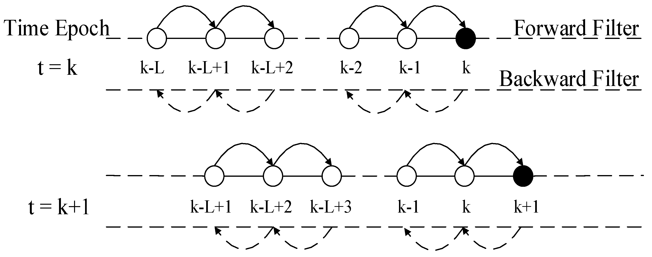
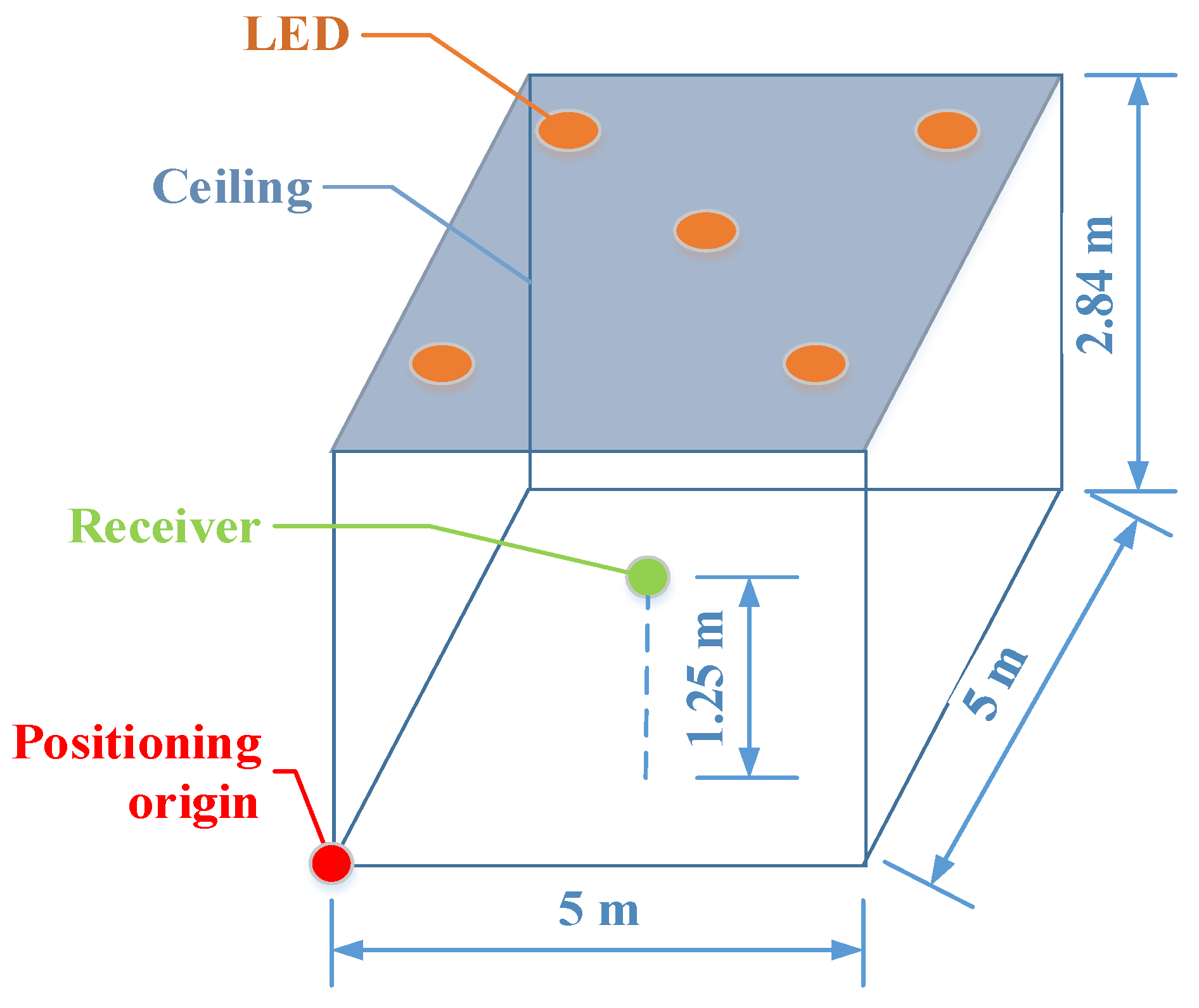
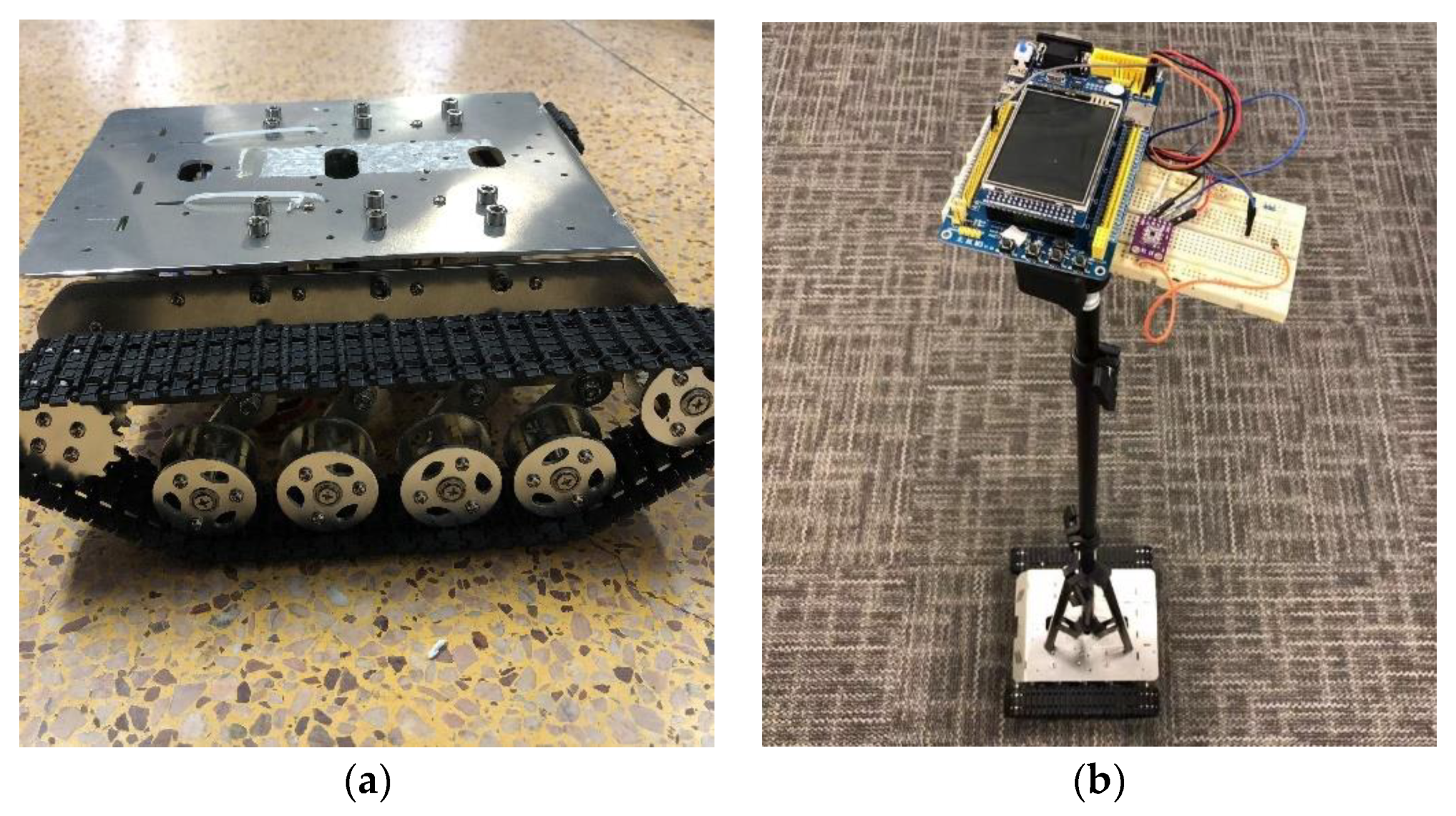
4.1. Experiment Setup

As shown in Figure 2, the size of the experiment area was 5 m × 5 m × 2.84 m. Five LEDs (CREE T6) were mounted evenly on the ceiling as light beacons. The power of each LED was 10 W, and the 3D coordinates of the LEDs in meters were (0.5, 0.5, 2.84), (2.5, 2.5, 2.84), (0.5, 4.5, 2.84), (4.5, 0.5, 2.84), and (4.5, 4.5, 2.84), respectively. An STM32 Microcontroller Unit (MCU) was applied to control the LEDs using Frequency Division Multiplexing (FDM) protocols.

In Figure 3, the receiver used in the experiments contained an OPT101 PD and a front camera of a smartphone. Two sensors were placed closely and mounted on a remotely controlled mobile robot at a height of 1.25 m. The parameters of the receiver are summarized in

Table 1. Receiver Parameters. PD: photodiode, FOV: field of view.

Receiver Parameters	Quantity
PD type	OPT101
FOV of PD	160 deg
PD area	5.2 mm2
Camera type	iPhone 5s front camera
FOV of camera	63.7 deg
Image pixel size	960 × 1280 px
Image resolution	72 dpi

. During the experiments, the robot moved along the pre-marked routes. Two different trajectories (i.e., rectangle and triangle) were tested to evaluate the dynamic performance of the proposed FLEnKS.

4.2. Results and Analyses

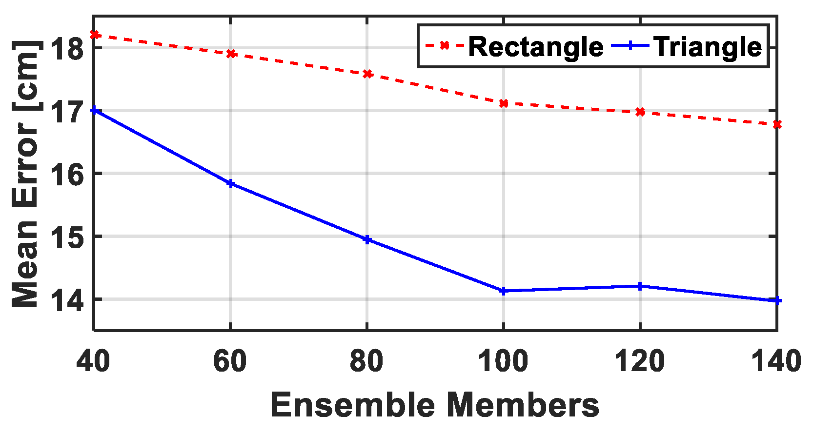
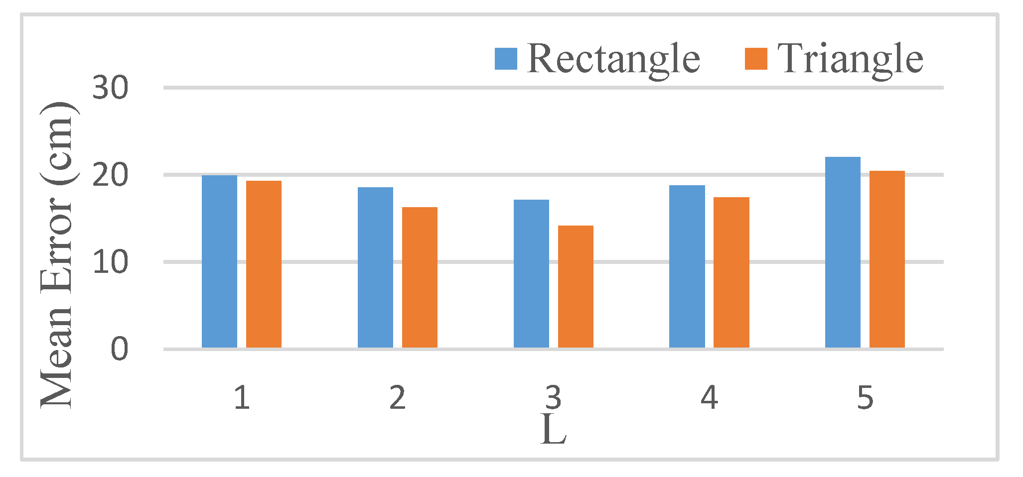
4.2.1. The Parameter Setup of FLEnKS

In the experiments, the time difference $\Delta t$ between two epochs was 0.5 s, which was limited by the frequencies of the LEDs and the analog-to-digital converter. In future work, $\Delta t$ will be configured to a shorter value by using a controller with higher performance. To evaluate the influence of the ensemble members on FLEnKS, different numbers of ensemble were selected with other parameters unchanged. The relationship between different ensemble members and the mean positioning errors of the FLEnKS can be seen in Figure 4. In Figure 4, with the increase of the ensemble members, the mean error is reduced. However, the improving rate slows down when the ensemble members are over 100. Thus, considering the trade-off between the accuracy and the complexity, the ensemble members were set to 100 in this research.

The performance of FLEnKS with different sizes of the analysis window (L) was also evaluated, and the relationship between different sizes of L and the mean positioning errors of the FLEnKS are shown in Figure 5. The maximum L was set to 5 in the evaluation, as the introduced latency by FLEnKS should be acceptable (<3 s).

In Figure 5, at the beginning, with the increase of the length of L, the mean positioning error is reduced as more measurements are fused in the smoother. However, when the analysis window size L > 3 (i.e., the analysis window is larger than 1.5 s as $\Delta t=0.5s$), the positioning measurements may vary largely. Thus, the measurements from a large analysis window will reduce the positioning accuracy. In the experiments, the size of the analysis window in FLEnKS was set to $L=3$, that is to say, the positioning results processed by FLEnKS had a positioning latency of 1.5 s during the experiments, which is acceptable for many semi-real applications.

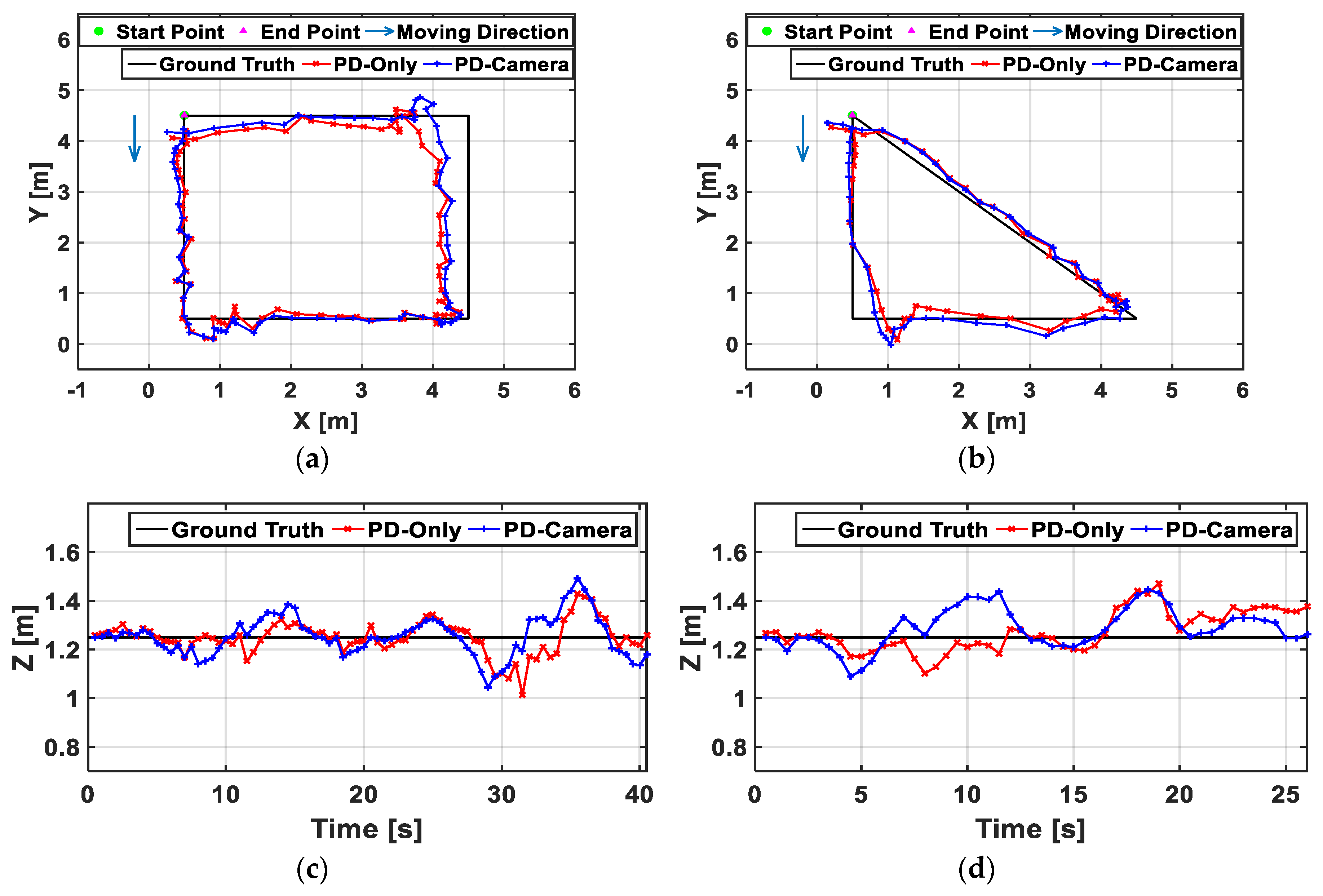
4.2.2. Comparison of PD-Only Positioning and PD–camera Data Fusion

To evaluate the performance of the PD–camera data fusion proposed in this article, two kinds of trajectories were tested based on PD-only positioning and PD–camera data fusion, respectively. Since this subsection focuses on the positioning performance by using different measured data, all the trajectories were processed by the proposed FLEnKS algorithm using PD-only and PD–camera measurements for better comparison. The 3D positioning results are depicted in Figure 6. The Mean Positioning Error (MPE) and Root-Mean-Square Error (RMSE) are shown in

Table 2. Positioning Errors of PD-Only Positioning and PD–Camera Data Fusion. MPE: Mean Positioning Error, RMSE: Root-Mean-Square Error.

Trajectory	MPE			RMSE
	PD-Only (cm)	PD–Camera (cm)	Improvement	PD-Only (cm)	PD–Camera (cm)	Improvement
Rectangle	21.85	17.12	21.65%	30.47	22.60	25.83%
Triangle	17.34	14.13	18.51%	21.54	17.56	18.48%

in detail.

As shown in Figure 6 and Table 2, both trajectories showed that PD–camera data fusion improved the positioning accuracy when compared to the PD-only positioning. The performance of PD-only positioning suffered from degradation in the corners. On the other hand, the measurements from the camera were more stable as they were obtained from the image features. Thus, PD–camera data fusion, which used the measurements from both PD and camera, achieved more accurate positioning performance.

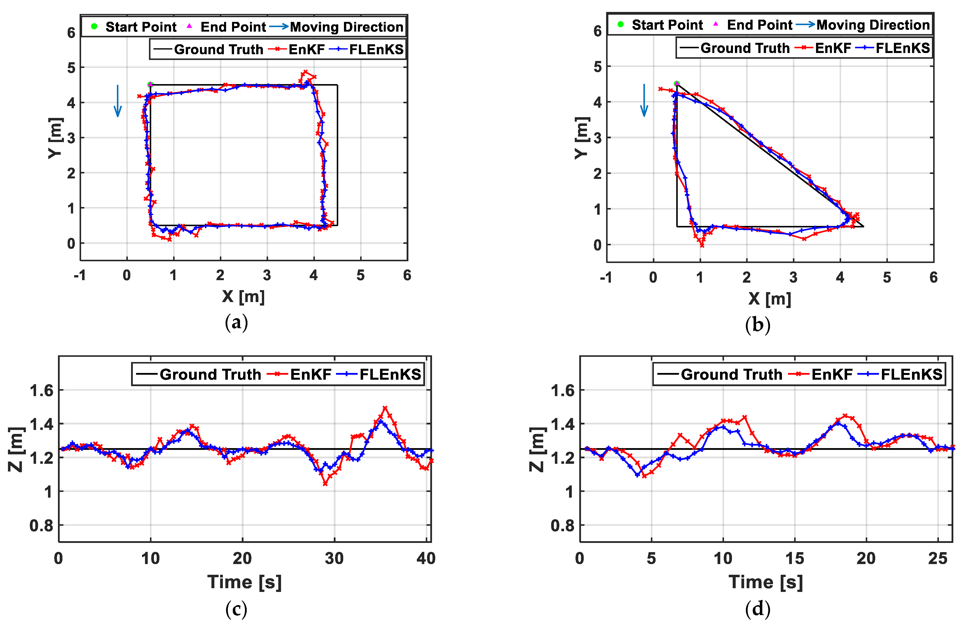
4.2.3. Comparison of EnKF and FLEnKS

To evaluate the performance of the proposed FLEnKS, it was compared with the traditional EnKF [23] to process two trajectories by using measurements from both PD and camera. The 3D positioning results by using FLEnKS and EnKF and both PD and camera measurements are shown in Figure 7. As shown in Figure 7, the positioning results using the FLEnKS were smoother and closer to the ground truth than those using the EnKF, especially at the corners. It is because the system states (e.g., speed) and noises (e.g., process noise and measurement noise) were significantly changed at the corner areas. When compared to the EnKF, FLEnKS applies a two-filter structure. The backward filter of FLEnKS reversely processes the data samples epoch by epoch to include the measurements after time k and compensates the estimation errors of the forward filter at time k. Thus, at the corner areas, the backward filter can integrate the measurements after the corner into the forward filter to better reduce the effects of the changed system states and noises. The two-filter FLEnKS provides a smoother estimation solution by using more measurements than the traditional filter algorithms and achieves better positioning results.

The MPE and RMSE of these two trajectories are summarized in

Table 3. Positioning Errors of EnKF and FLEnKS.

Trajectory	MPE			RMSE
	EnKF (cm)	FLEnKS (cm)	Improvement	EnKF (cm)	FLEnKS (cm)	Improvement
Rectangle	18.96	17.12	9.70%	23.84	22.60	5.20%
Triangle	16.93	14.13	16.54%	20.63	17.56	14.88%

. The MPEs of the FLEnKS were 9.70% and 16.54% lower than the those of EnKF in the rectangle and triangle trajectory, respectively. Furthermore, the RMSEs of EnKF were reduced by 5.20% and 14.88%, respectively, in two trajectories when the FLEnKS was adopted.

4.2.4. Comparison of FLEnKS with Existing Fixed-lag Smoothers

To further evaluate the performance of the proposed FLEnKS, other fixed-lag smoothers proposed in previous works were applied to the VLP system in this article using both PD and camera measurements. The evaluated smoothers included the FLEKS in [11], the FLSPKS proposed in [13], and the FLEnKS proposed in this article.

As shown in

Table 4. MPE and RMSE of Different Smoothers. FLEKS: Fixed-Lag Extended Kalman Smoother, FLSPKS: Fixed-Lag Sigma-Point Kalman Smoother.

	Rectangle (cm)		Triangle (cm)		Average (cm)
	MPE	RMSE	MPE	RMSE	MPE	RMSE
FLEKS [11]	23.77	30.66	23.00	27.50	23.39	29.08
FLSPKS [13]	22.27	26.89	19.66	23.28	20.97	25.09
FLEnKS	17.12	22.60	14.13	17.56	15.63	20.08

, the positioning results using the FLEnKS consistently outperformed those obtained with the other smoothers. The EKF converts the nonlinear model into an approximate linear model through Taylor series expansion, which produces truncated errors. The SPKF is a deterministic sampling algorithm with certain sample points to reflect the nonlinear model. On the other hand, the EnKF using stochastic sampling with more ensemble members can better reflect the features of a nonlinear system and get better estimates than the EKF and SPKF. Thus, the FLEnKS using the EnKF as a forward filter can achieve better positioning results than the FLEKS and FLSPKS, which are based on EKF and SPKF, respectively. Furthermore, the backward filter of the two-filter FLEnKS is based on the error state vectors, while the FLEKS and FLSPKS use normal state vectors. The consideration of error states will be more suitable for applications focusing on errors, such as positioning.

Considering the average MPE in the two trajectories, the MPE of FLEnKS was 33.18% and 25.47% lower than those of FLEKS and FLSPKS, respectively. Furthermore, the RMSE of FLEnKS was 30.95% and 19.95% lower than those of FLEKS and FLSPKS, respectively. Overall, the proposed FLEnKS achieved the best positioning performance, and the average 3D positioning accuracy was 15.63 cm in two trajectories with PD–camera data fusion.

4.2.5. Evaluation of Different Speeds

To evaluate the performance of FLEnKS at different speeds, extra experiments were conducted at a speed around 0.5 m/s faster and a speed around 0.5 m/s slower than those in the previous experiments. The MPE and RMSE at three different speeds are summarized in

Table 5. MPE and RMSE at Different Speeds.

	Rectangle (cm)		Triangle (cm)		Average (cm)
	MPE	RMSE	MPE	RMSE	MPE	RMSE
Fast	18.46	24.50	14.48	18.26	16.47	21.38
Medium	17.12	22.60	14.13	17.56	15.63	20.08
Slow	16.98	22.98	13.55	17.58	15.27	20.28

.

In Table 5, the FLEnKS was applied to the VLP system using both PD and camera measurements at different speeds, and the medium speed means the positioning results mentioned in Section 4.2.2, Section 4.2.3 and Section 4.2.4. The MPE results showed that positioning accuracy was increased when the speed was lower. Since the time difference $\Delta t$ stayed unchanged during the tests, a slower speed would produce more stable system measurements and provide better positioning results. However, the MPE and RMSE results imply that the speed difference was not a significant factor affecting the positioning accuracy.

4.2.6. Comparison of Existing VLP Systems

Table 6. Comparison of the Proposed Visible Light Positioning (VLP) System with Other Existing Systems.

System	Experiment/Simulation	Test Bed Size	Method	Receiver	Mean Error
[24]	Simulation	2 m × 10 m	RSS + AOA + EKF	PD array	20 cm (2D)
[25]	Experiment	3.5 m × 6.5 m	RSS	PD	30 cm (2D)
[26]	Experiment	5 m × 3 m × 3 m	RSS + AOA	PD + Accelerometer	25 cm (3D)
Ours	Experiment	5 m × 5 m × 2.84 m	RSS + FLEnKS	PD + Camera	15.63 cm (3D)

shows the comparison of the VLP system proposed in this article with other related systems. As shown in Table 6, our proposed VLP system based on FLEnKS achieved better 3D positioning results with an ordinary PD and a low-cost camera.

5. Conclusions

The FLEnKS proposed in this article is a semi-real-time smoother, which can meet the requirements for many positioning, localization, and tracking systems and improve their positioning accuracy. The forward part of the FLEnKS is based on stochastic sampling with ensemble members, which enables a better reflection of the features of nonlinear systems and better estimates than the smoothers based on SPKF using deterministic sampling with certain samples and EKF using Taylor series expansion. The backward filter in the FLEnKS compensates for the estimation error from the forward filter using the linearization based on error states and further reduces the estimation error. The proposed FLEnKS was practically evaluated in the VLP system by fusing the measurements from PD and camera, and preliminary experimental results showed the proposed FLEnKS improved the 3D positioning accuracy by 33.18% and 25.47% when compared to FLEKS and FLSPKS, respectively. Meanwhile, the fusion of PD and camera measurements improved the average positioning accuracy by 20.08% when compared to PD-only schemes. The experiments in the article were conducted in a 5 m × 5 m × 2.84 m area, which is the normal size for evaluating VLP systems. A larger positioning area will be evaluated in future work, considering obstruction and interference problems.

References

1. Zhuang, Y.; Hua, L.; Qi, L.; Yang, J.; Cao, P.; Cao, Y.; Wu, Y.; Thompson, J.; Haas, H. A Survey of Positioning Systems Using Visible LED Lights. IEEE Commun. Surv. Tutor. 2018, 20, 1963–1988. [Google Scholar] [CrossRef] [Green Version]
2. Zhou, B.; Lau, V.; Chen, Q.; Cao, Y. Simultaneous Positioning and Orientating for Visible Light Communications: Algorithm Design and Performance Analysis. IEEE Trans. Veh. Technol. 2018, 67, 11790–11804. [Google Scholar] [CrossRef]
3. Zhuang, Y.; El-Sheimy, N. Tightly-coupled integration of WiFi and MEMS sensors on handheld devices for indoor pedestrian navigation. IEEE Sens. J. 2016, 16, 224–234. [Google Scholar] [CrossRef]
4. Xu, Y.; Tian, G.; Chen, X. Enhancing INS/UWB Integrated Position Estimation Using Federated EFIR Filtering. IEEE Access 2018, 6, 64461–64469. [Google Scholar] [CrossRef]
5. Zhuang, Y.; Yang, J.; Qi, L.; Li, Y.; Cao, Y.; El-Sheimy, N. A Pervasive Integration Platform of Low-Cost MEMS Sensors and Wireless Signals for Indoor Localization. IEEE Internet Things J. 2017, 5, 4616–4631. [Google Scholar] [CrossRef]
6. Li, Y.; Zhuang, Y.; Lan, H.; Zhang, P.; Niu, X.; El-Sheimy, N. Self-Contained Indoor Pedestrian Navigation Using Smartphone Sensors and Magnetic Features. IEEE Sens. J. 2016, 16, 7173–7182. [Google Scholar] [CrossRef]
7. Li, Y.; He, Z.; Gao, Z.; Zhuang, Y.; Shi, C.; El-Sheimy, N. Toward Robust Crowdsourcing-Based Localization: A Fingerprinting Accuracy Indicator Enhanced Wireless/Magnetic/Inertial Integration Approach. IEEE Internet Things J. 2019, 6, 3585–3600. [Google Scholar] [CrossRef]
8. Nassar, S.; Niu, X.; El-Sheimy, N. Land-vehicle INS/GPS accurate positioning during GPS signal blockage periods. J. Surv. Eng. 2007, 133, 134–143. [Google Scholar] [CrossRef]
9. Zhuang, Y.; Wang, Q.; Shi, M.; Cao, P.; Qi, L.; Yang, J. Low-Power Centimeter-Level Localization for Indoor Mobile Robots Based on Ensemble Kalman Smoother Using Received Signal Strength. IEEE Internet Things J. 2019. [Google Scholar] [CrossRef]
10. Bruhwiler, L.; Michalak, A.; Peters, W.; Baker, D.; Tans, P. An improved Kalman Smoother for atmospheric inversions. Atmos. Chem. Phys. 2005, 5, 2691–2702. [Google Scholar] [CrossRef] [Green Version]
11. Cosme, E.; Verron, J.; Brasseur, P.; Blum, J.; Auroux, D. Smoothing Problems in a Bayesian Framework and Their Linear Gaussian Solutions. Mon. Weather Rev. 2010, 140, 683–695. [Google Scholar] [CrossRef]
12. Xu, Y.; Chen, X.; Li, Q. Autonomous Integrated Navigation for Indoor Robots Utilizing On-Line Iterated Extended Rauch-Tung-Striebel Smoothing. Sensors 2013, 13, 15937–15953. [Google Scholar] [CrossRef] [Green Version]
13. Paul, A.S.; Wan, E.A. RSSI-Based Indoor Localization and Tracking Using Sigma-Point Kalman Smoothers. IEEE J. Sel. Top. Signal Process. 2009, 3, 860–873. [Google Scholar] [CrossRef]
14. Merwe, R.; Wan, E. Sigma-Point Kalman Filters for Probabilistic Inference in Dynamic State-Space Models. In Proceedings of the Workshop on Advances in Machine Learning, Montreal, QC, Canada, 8–11 June 2003. [Google Scholar]
15. Guimaraes, A.G.; Fquih, B.A.E.; Desbouvries, F. A fixed-lag particle smoothing algorithm for the blind turbo equalization of time-varying channels. In Proceedings of the IEEE International Conference on Acoustics, Speech and Signal Processing, Las Vegas, NV, USA, 31 March–4 April 2008; pp. 2917–2920. [Google Scholar]
16. Cosme, E.; Brankart, J.M.; Verron, J.; Brasseur, P.; Krysta, M. Implementation of a reduced rank square-root smoother for high resolution ocean data assimilation. Ocean Model. 2010, 33, 87–100. [Google Scholar] [CrossRef]
17. Gupta, S.D. A Comparative Study of the Particle Filter and the Ensemble Kalman Filter. Master’s Thesis, University of Waterloo, Waterloo, ON, Canada, 2009. [Google Scholar]
18. Merwe, R.V.D. Sigma-Point Kalman Filters for Probabilistic Inference in Dynamic State-Space Models. Ph.D. Thesis, Oregon Health & Science University, Portland, OR, USA, 2004. [Google Scholar]
19. Liu, H.; Nassar, S.; El-Sheimy, N. Two-Filter Smoothing for Accurate INS/GPS Land-Vehicle Navigation in Urban Centers. IEEE Trans. Veh. Technol. 2010, 59, 4256–4267. [Google Scholar] [CrossRef]
20. Gong, X.; Zhang, J.; Fang, J. A Modified Nonlinear Two-Filter Smoothing for High-Precision Airborne Integrated GPS and Inertial Navigation. IEEE Trans. Instrum. Meas. 2015, 64, 3315–3322. [Google Scholar] [CrossRef]
21. Crassidis, J.L.; Junkins, J.L. Optimal Estimation of Dynamic Systems; Chapman Hall/CRC: Boca Raton, FL, USA, 2011. [Google Scholar]
22. Saeedi, S.; Moussa, A.; Elsheimy, N. Context-Aware Personal Navigation Using Embedded Sensor Fusion in Smartphones. Sensors 2014, 14, 5742–5767. [Google Scholar] [CrossRef] [PubMed]
23. Gillijns, S.; Mendoza, O.B.; Chandrasekar, J.; de Moor, B.; Bernstein, D.; Ridley, A. What is the ensemble Kalman filter and how well does it work. In Proceedings of the 2006 American Control Conference, Minneapolis, MN, USA, 14–16 June 2006. [Google Scholar]
24. Nguyen, N.T.; Nguyen, N.H.; Nguyen, V.H.; Sripimanwat, K.; Suebsomran, A. Improvement of the VLC localization method using the Extended Kalman Filter. In Proceedings of the TENCON 2014—2014 IEEE Region 10 Conference, Bangkok, Thailand, 22–25 October 2014; pp. 1–6. [Google Scholar]
25. Li, L.; Hu, P.; Peng, C.; Shen, G.; Zhao, F. Epsilon: A visible light based positioning system. In Proceedings of the 11th USENIX Symposium on Networked Systems Design and Implementation (NSDI 14), Seattle, WA, USA, 2–4 April 2014; pp. 331–343. [Google Scholar]
26. Yasir, M.; Ho, S.-W.; Vellambi, B.N. Indoor Positioning System Using Visible Light and Accelerometer. J. Lightwave Technol. 2014, 32, 3306–3316. [Google Scholar] [CrossRef]
Figure 1. The process of the fixed-lag ensemble Kalman smoother (FLEnKS) algorithm.
Remotesensing 11 01387 g001
Figure 2. Experiment Setup.
Remotesensing 11 01387 g002
Figure 3. The mobile robot and receiver module: (a) Mobile robot and (b) Receiver module installed on the mobile robot.
Remotesensing 11 01387 g003
Figure 4. The relationship between positioning accuracy and ensemble members.
Remotesensing 11 01387 g004
Figure 5. The relationship between positioning accuracy and analysis window (L) size.
Remotesensing 11 01387 g005
Figure 6. The estimated trajectories based on PD-only positioning and PD–camera data fusion. (a) Rectangle trajectory, (b) Triangle trajectory, (c) Rectangle Z-axis results, and (d) Triangle Z-axis results.
Remotesensing 11 01387 g006
Figure 7. The estimated trajectories based on FLEnKS and Ensemble Kalman Filter (EnKF). (a) Rectangle trajectory, (b) Triangle trajectory, (c) Rectangle Z-axis results, and (d) Triangle Z-axis results.
Remotesensing 11 01387 g007