Changes in SO₂ Flux Regime at Mt. Etna Captured by Automatically Processed Ultraviolet Camera Data

Abstract

We used a one-year long SO₂ flux record, which was obtained using a novel algorithm for real-time automatic processing of ultraviolet (UV) camera data, to characterize changes in degassing dynamics at the Mt. Etna volcano in 2016. These SO₂ flux records, when combined with independent thermal and seismic evidence, allowed for capturing switches in activity from paroxysmal explosive eruptions to quiescent degassing. We found SO₂ fluxes 1.5–2 times higher than the 2016 average (1588 tons/day) during the Etna’s May 16–25 eruptive paroxysmal activity, and mild but detectable SO₂ flux increases more than one month before its onset. The SO₂ flux typically peaked during a lava fountain. Here, the average SO₂ degassing rate was ~158 kg/s, the peak emission was ~260 kg/s, and the total released SO₂ mass was ~1700 tons (in 3 h on 18 May, 2016). Comparison between our data and prior (2014–2015) results revealed systematic SO₂ emission patterns prior to, during, and after an Etna’s paroxysmal phases, which allows us to tentatively identify thresholds between pre-eruptive, syn-eruptive, and post-eruptive degassing regimes.

1. Introduction

Active volcanoes are monitored by a variety of increasingly sophisticated volcanic gas sensing techniques [1,2,3], which are contributing to improved understanding and monitoring of volcanic activity. In particular, trends in volcanic gas composition and fluxes help detect subtle changes in the rates of magma ascent and degassing within shallow volcano plumbing systems, and allow to better confinepre-eruptive and syn-eruptive processes (gas in magmas being the main drivers of volcanic processes) [4]. Nevertheless, gas monitoring still lags behind more established seismic and geodetic techniques [5]. This is because the low temporal resolution of gas observations has traditionally hampered real-time analysis of fast-occurring volcanic processes, such as shallow intrusion of magma prior to eruption, and rapid gas ascent and release during explosive eruptions.

Volcanic SO₂ emissions provide key information on the rates of magma ascent in shallow (<3 km) magma plumbing systems, and are extensively monitored worldwide using instrumental networks of scanning ultraviolet spectrometers using the Differential Optical Adsorption Spectroscopy (DOAS) technique [6]. The advantage of this method is that acquisition and processing are relatively easy to automate [7], which yield exceptionally continuous records of volcanic SO₂ fluxes at relatively high temporal resolution (tens of minutes) [8,9,10]. Biases in the technique include limited spatial resolution (making it impossible to distinguish contemporaneous degassing from different vents), temporal resolution inadequate to resolve individual explosive events, and errors related to poor knowledge of plume speed [11].

The recent advent of UV cameras [12] has paved the way to volcanic SO₂ flux observations of much improved temporal and spatial resolution (see References [13,14,15] for recent reviews), which contributes to more effective integration between gas and geophysical datasets [16,17,18,19,20,21,22,23,24,25,26,27,28,29].

Even though space-based techniques are becoming increasingly performant in detecting volcanic SO₂ fluxes, ground-based SO₂ flux observations are still important and fundamental in monitoring basaltic volcanoes. While satellites become invaluable during paroxysmal explosive eruptions, when measurements from ground are complicated by volcanic ash within the plume. UV-camera measurements are more effective in monitoring more sluggish quiescent emissions in the low troposphere, and perhaps more useful to capture the early phases of unrest with escalating degassing activity [30].

The first examples of fully automated, permanent UV camera systems [14,28,31,32] are particularly promising, since they are opening the way to routinely monitoring volcanic SO₂ flux at a high rate continuously (daily hours only). For example, Reference [32] has demonstrated the ability of UV cameras to capture a precursory phase of heightened SO₂ flux in the weeks prior to the 2014 effusive eruption at the Stromboli volcano (Italy).

A current limitation of permanent UV camera systems is that, while data acquisition is fully autonomous, data processing is still time-consuming and operator-managed, e.g., data streamed by these systems are archived, and post-processed with ad-hoc codes [33]. To fully exploit the volcano monitoring potentials of UV cameras, automation of UV camera acquisition and processing routines is now timely and important.

The objectives of this study are: (i) to describe a new automatic routine for nearly real-time processing and visualization of UV camera data, (ii) to demonstrate the ability of the automatic routine to capturing temporal changes in SO₂ flux regime at Mt. Etna, and (iii) to contribute to better constraining Etna’s degassing and eruptive behavior in 2016. To this aim, we reported on automatically processed data streamed by a permanent UV camera deployed on Etna. In order to fully characterize the Etna’s 2016 behavior, we integrated our SO₂ flux results with independent geophysical parameters, traditionally used at Mt. Etna to constrain volcanic activity state and evolution [34,35,36,37,38,39,40,41,42]. More specifically, we used Moderate Resolution Imaging Spectroradiometer (MODIS) satellite-based thermal data obtained from the MIROVA (Middle InfraRed Observation of Volcanic Activity) system [43], ground-based thermal data streamed by monitoring cameras [44] of the Osservatorio Etneo (INGV-OE), and seismic tremor data [34,36,42].

2. Materials and Methods

2.1. UV Camera System

In the framework of the ERC-funded project BRIDGE (www.bridge.unipa.it), we designed a multi-instrument UV-absorption spectroscopy system for robust SO₂ flux measurements (Figure S1). The system is composed of (i) an instrument module and (ii) an acquisition/processing module. The instrument module is equipped with two JAI CM-140GE-UV cameras sensible to UV-radiation, and one Ocean-Optics USB2000+ Spectrometer coupled to a telescope of rectangular, vertically-oriented Field Of View (FOV ≈ 0.3° × 14°), and is spatially filtered to match the ≈12° vertical width. Two different band-pass optical filters with Full Width at Half Maximum (FWHM) of 10 nm, and a central wavelength of 310 and 330 nm, respectively, are applied in front of the cameras to enhance differential UV absorption in the SO₂ bandwidth [45,46]. In addition, 520 × 676 pixel images are acquired at 10-bit resolution with a frame rate of 0.5 Hz.

To obtain a quantitative measure of SO₂ column density within the volcanic cloud, we calculate the proportionality ratio between absorbance and SO₂ concentration in a defined region of the image pointed by the Ocean-Optic USB2000+ Spectrometer [47]. The use of the UV spectrometer allows us to quantitatively measure the full UV spectrum, and then fit the theoretical SO₂ absorption cross-section [48] with the differential absorption between two consecutive spectra (acquired every 5 seconds). The Ocean-Optic USB2000+ Spectrometer in use has on-board a Sony ILX511B Linear Silicon CCD Array Detector at 2048 pixels, with a wavelength response of 200–1100 nm, a dynamic range of 8.5 × 108, and a SNR of 250:1 at full signal. Calibrated SO₂ column densities over the entire images are then obtained by integrating images achieved by the UV camera with information achieved by the spectrometer. The instrument module is powered with a 12 V power supply, and requires 15 W in a fully operational mode. A Fujitsu RX100 Workstation, connected to the instrument module, automatically acquires synchronous data from the instrument module, and processes data without the need of the operator. To do this, we designed algorithms to control acquisition and processing parameters, such as the automatic tuning of camera’s and spectrometer’s exposures, and automatic evaluation of optimal viewing conditions (see Section 2.3.2). The computer internal time drift is controlled by a specifically designed application that reads the time-stamp from an NMEA (National Marine Electronics Association) standard message coming from a GPS antenna. The instrument module communicated with the acquisition/processing module via wired or wireless TCP/IP connection.

This UV camera system was installed at the Montagnola site (on Etna Volcano, Figure 1), and designed to stream real-time SO₂ flux results using a Wi-Fi data link. The objective is to capture SO₂ emissions associated with diverse volcanic processes and dynamics, including quiescent (passive) degassing, explosive eruptions (strombolian activity/lava fountaining), and effusive eruptions [49]. Montagnola is located at ~3 km distance from the active summit vents and grants perfect views of the southern sector of the summit crater area (Figure 1).

2.2. Seismic and Thermal Data

We compared our SO₂ fluxes with other independent geophysical parameters such as tremor and thermal radiance primary to have a benchmark in the calibration of automatic SO₂ flux calculation algorithm. Last but not least, we combined these data to characterize volcanic activity.

We used seismic data recorded by the ETN station [42,50], located at Lapide Malerba, at 5 km from the summit area. ETN is equipped with a broad-band seismometer (Guralp CMG-40T, with a sensitivity of 800 V/(m/s) and eigen period of 30 s). The link between SO₂ flux and volcanic tremor at Mt. Etna [22,51,52] suggests that the tremor is generated by the same degassing dynamics. We then calculated volcanic tremor amplitude from raw traces recorded at ETN station, by averaging within a 1-minute length window the maximum RMS amplitude taken within a 1-s window.

Thermal remote sensing offers a great opportunity to follow volcanic unrest from ground and space to characterize volcanic activity in near-real time [53] and to estimate near vent large pyroclastic products and lava flow discharged during eruptions. We used satellite data from the MIROVA system [43,54] and ground-based thermal cameras [44] to constrain onset, duration, and intensity through the time of eruptive events occurring at Etna during 2016. In particular, MIROVA uses the data provided by the MODIS sensor, which acquires four images per day (two daytime and two nighttime) with a spatial resolution of 1 km in the infrared bands [43]. The heat flux retrieved from MIROVA data, called Volcanic Radiative Power (VRP), is a combined measurement of the area and the integrated temperature of the hot emitters (hot vents, lava flows, etc.) at the time of each image acquisition. These data are provided without correction for cloud cover and satellite view geometry [43]. These factors may introduce noise in the dataset, which has been proven not to affect the general trend associated with the activity of Mt. Etna [43]. A mask 5 × 5 km around the volcano summit is used to filter out thermal anomalies due to wildfires.

2.3. The Algorithm for Automatic Processing of UV Camera Data

Manual processing of UV camera results [33] has the advantage that images are checked and validated manually by an operator. However, manual procedures are time-consuming, especially when dealing with huge data flows from permanent monitoring stations. To overcome this limit, we designed a MATLAB-based algorithm to automatically process images, and thus obtain SO₂ fluxes in near real-time. Using a “low-cost” PC-workstation (with 8 GB RAM and Xeon E3 type CPU), we can successfully process data at ~5× speed (i.e., a 5 minutes-long record is processed in ~1 min), which allows nearly real-time monitoring. The automatic routine has been calibrated using the results of the manual procedure and includes: (1) automatic determination of background absorbance levels, (2) automatic determination of image goodness, using image quality indexes, (3) estimation of gas plume speed and its distribution across the crater area, and (4) calculation of SO₂ flux distribution throughout the summit crater area. These are described in more detail below.

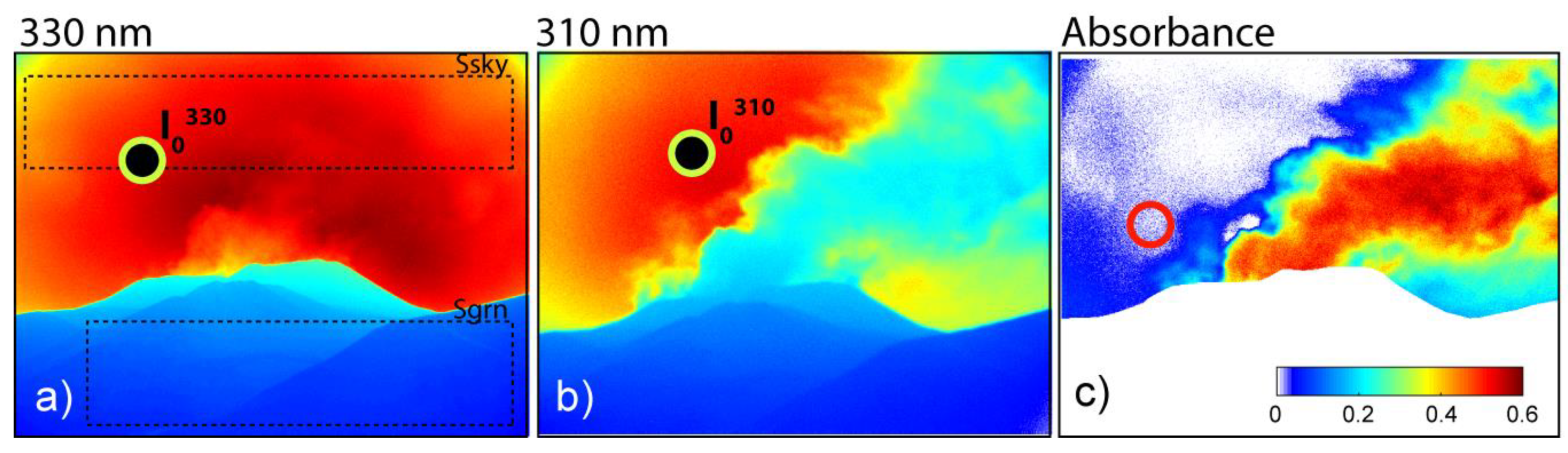
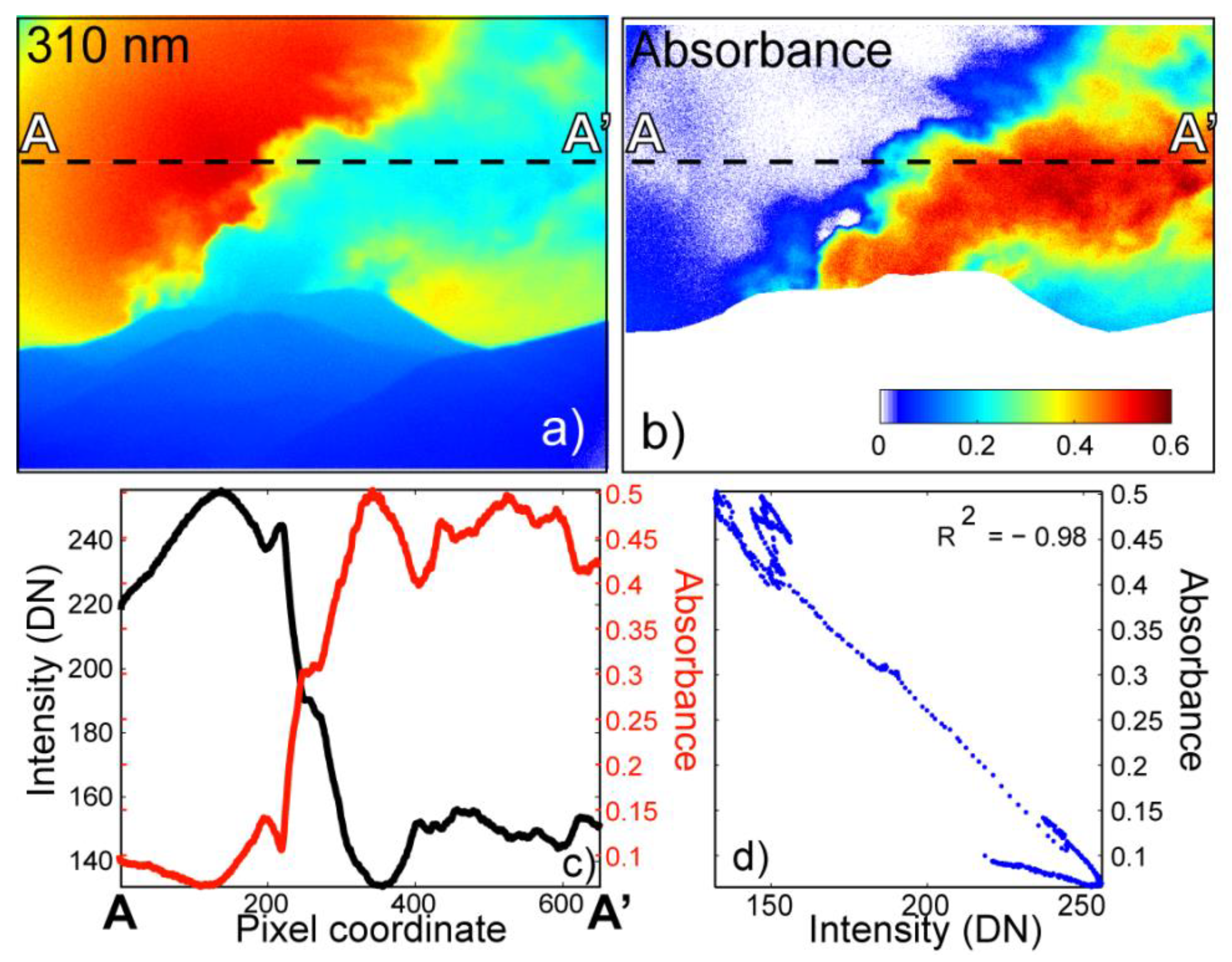
2.3.1. Image Processing and SO₂ Column Densities

Relative UV absorption by volcanic plume SO₂ is quantified by applying the Beer–Lambert law. Sets of synchronous images, taken by the two co-aligned cameras using different filters, are combined to obtain single absorbance images. This method, known as the “double filter method” [12,45], implies the use of two cameras with different filters, with one centered at 310 nm and the other centered on 330 nm, where UV radiation is/is not absorbed, respectively. The use of the two filters method allows compensating for aerosol attenuation/backscattering, to avoid any temporal mismatch associated with filter change while using a single camera, and to maintain the sampling rate at up to 0.5 Hz (two synchronous images every 2 s taken by two cameras [45]).

In our automatic routine, once a new raw image is acquired, a first quality check is made by the system, in order to keep the best exposure times to compensate any subtle changes in sunlight intensity. An automatic real-time tuning of exposure time is also applied to the UV spectrometer data, in order to obtain the best measurement dynamics within the UV bandwidth.

Synchronous images from the two cameras are then real-time corrected for vignetting effects associated with filters and optics, and normalized for relative exposure times. Residual intensities are then combined to obtain an un-calibrated absorbance image using the Lambert-Beer Law equation.

$$A=-{\log }_{10}\frac{I^{310}}{I^{330}}-A_0$$

(1)

where A is the absorbance, I³¹⁰ and I³³⁰ are pixel intensities associated with cameras mounting the 310 or 330 nm filter, while A₀ is the absorbance level associated with a clear background sky sub-area of the image (assumed to be unaffected by SO₂ absorption, I₀³¹⁰ and I₀³³⁰ of Figure 2) and calculated as −log₁₀(I³¹⁰/I³³⁰), following Kern [55].

In the automatic processing module, this background sky sub-area is automatically selected for each image by monitoring a distal sky horizontal section with respect to the vent position, and selecting the sector with the lowest absorbance intensity.

Residual absorbance is then converted into SO₂ column density integrating data from the co-located ultraviolet spectrometer, which is pointing to a known sub-area within the camera field of view. This procedure yields, in real-time, the proportionality ratio between absorbance and SO₂ column densities using the method described in McGonigle [47].

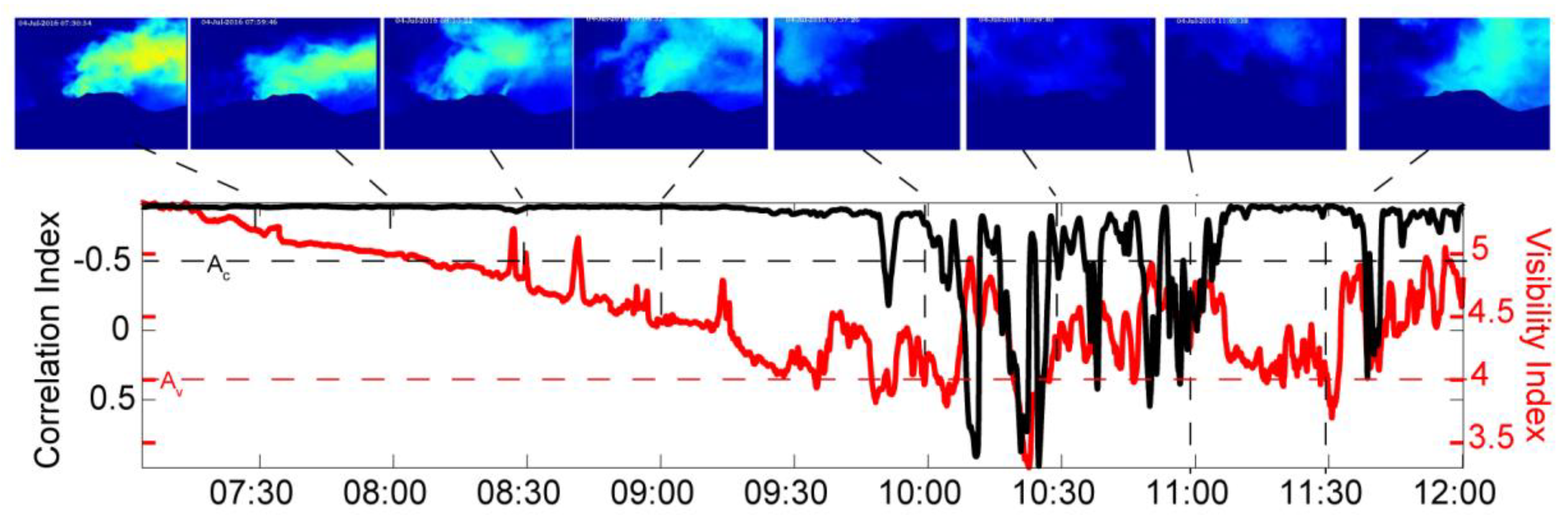
2.3.2. Automatic Determination of the Optimal Viewing Condition

The optimal plume viewing conditions, and the presence of a clear sky, are required for reliable SO₂ density measurements. However, weather conditions are extremely variable on Etna’s summit, and often prevent optimal SO₂ observation. To minimize uncertainties due to poor weather conditions, we set-up a sub-routine for real-time calculation of two visibility indexes. The first visibility index (Fog index) is calculated as the unsigned ratio between the mean pixel intensity associated with the camera FOV’s portions capturing sky and ground, respectively. Tests we conducted on real and synthetic images show that the higher this ratio is, the better the visibility condition is. SO₂ measurements are then selected by setting a threshold on the visibility index, and discarding measurements below the threshold (e.g., biased by a poor visibility condition).

Detecting a “sky” signal well above the “ground” signal (Figure 2) is a required but not sufficient condition for reliable SO₂ measurements. This is especially true in the presence of a highly condensed plume, where the SO₂ absorbance signal can be masked. Thus, a second automatic procedure was developed and run in real-time, which allows us to select only images with a clear SO₂ signal above atmospheric noise.

This latter procedure is based on the principle of combining absorbance and 310 nm images associated with the plume. A well detected and measurable SO₂ signal requires that lower intensities in the 310 nm image are measured in the plume relative to its surroundings (because SO₂ is absorbing solar radiation), and that higher intensities are consistently obtained in the absorbance image (see the Lambert Beer equation). This condition is only verified if the SO₂ signal is high enough to emerge above the atmospheric noise. To discriminate this condition in real-time, we defined a correlation index (Figure 3) as the correlation coefficient between absorbance and 310-nm pixel intensities over a cross-section intersecting the plume (Figure 3 and Figure 4). The correlation coefficient is defined as C(i,j)/((C(i,i)*C(j,j))^(1/2), where C is the covariance matrix, i and j are pixel intensities over the cross-section of absorbance and 310-nm images, respectively. In such plots, the closer the correlation coefficient is to the value -1, the more absorbance can be related to gas. Images that do not satisfy this condition (e.g., that have a Correlation Index < −0.5) are disregarded by the automatic computation (Figure 4).

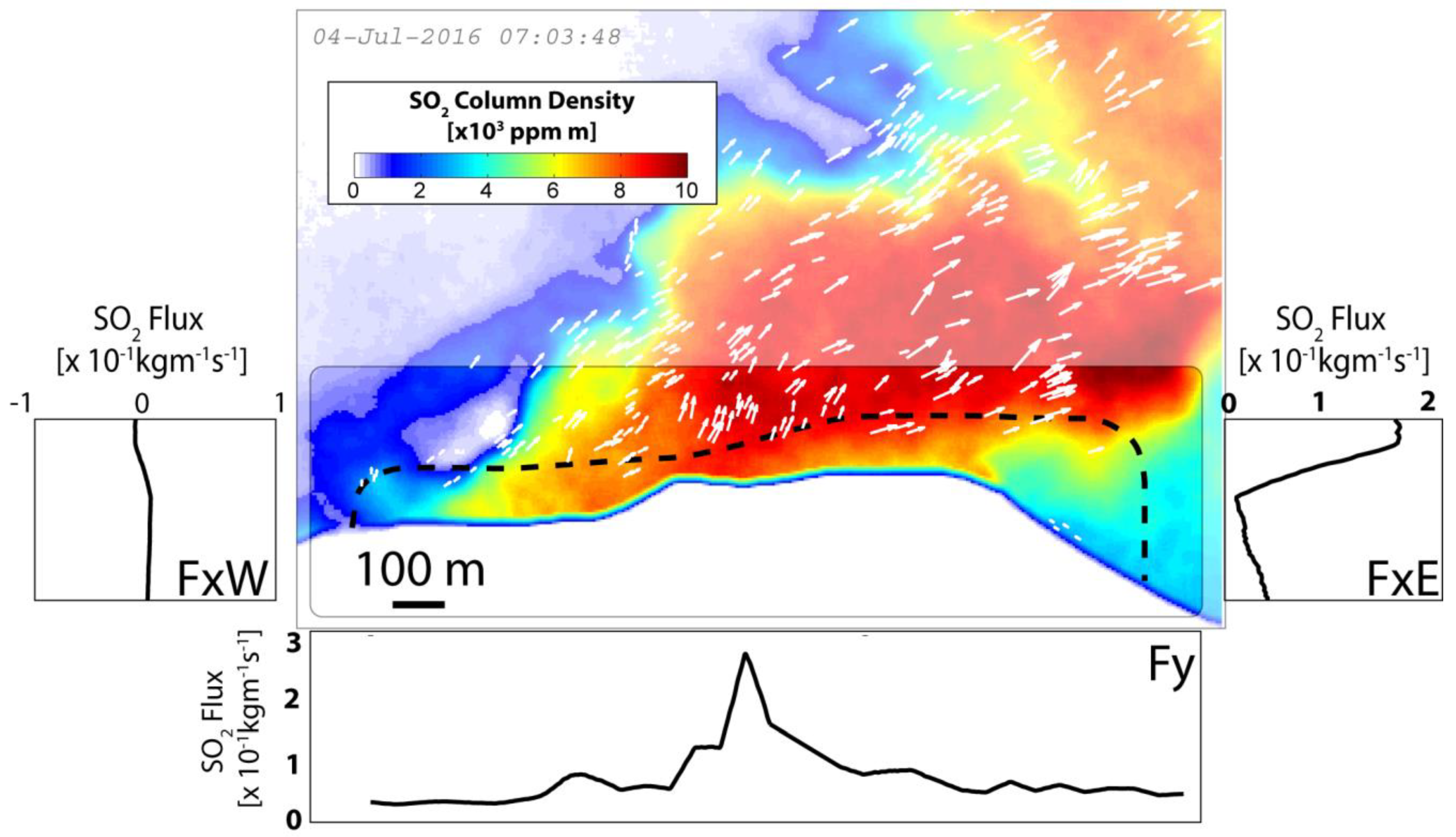
2.3.3. Plume Velocity Field

A robust plume velocity field is mandatory for reliable SO₂ flux measurements. Errors in plume velocity have shown to contribute to 40% or more of the overall error in the determined fluxes [13,57].

The UV camera approach offers the unique opportunity to track the gas while dispersing right after atmospheric emission, which minimizes errors in plume speed determination of yet more established DOAS and COSPEC methods. These methods indirectly infer plume speed from either on-site measurement of wind velocity or from meteorological models [11,15].

The UV camera approach allows us to derive the velocity profile over the summit craters by applying an optical flow algorithm that tracks gas fronts in consecutive frames [58].

Optical flow consists ofthe apparent motion pattern of image objects between two consecutive frames, caused by the movement of either the object or the camera, and is valid under the assumptions that the pixel intensities of an object do not change significantly between consecutive frames, and that the neighboring pixels have similar motion.

If a pixel, with intensity I(x,y,t), where (x,y) are the pixel coordinates and t is the time in first frame, moves by distance (dx,dy) in the next frame taken after time dt, it can be assumed that:

$$I\left(x,y,t\right)=I\left(x+dx,y+dy,t+dt\right)$$

(2)

Then, from the Taylor series approximation of the right-hand side, removing common terms and dividing by dt, one gets the following equations.

$$\frac{\partial I}{\partial x}u+\frac{\partial I}{\partial y}v+\frac{\partial I}{\partial t}=0$$

(3)

$$u=\frac{dx}{dt};v=\frac{dy}{dt}$$

(4)

where $\frac{\partial I}{\partial x}$ and $\frac{\partial I}{\partial y}$ are the image gradients, $\frac{\partial I}{\partial t}$ is the gradient along time, and u and v are horizontal and vertical velocities that are unknown. Lucas & Kanade [59] provide a method (LK) to derive these unknown velocities, by solving the basic optical flow Equations (3) and (4) for all the pixels using the least squares criterion, and by combining information from nearby pixels. We then applied the LK algorithm, included within the Open-CV toolbox, to our dataset [60]. We tested the performance of this method by applying it to artificial images with known particle velocities. The method has successfully determined velocity field with an error of <5%.

Absorbance images, obtained using the two filters method, contain gas-rich and ash-free portions of the plume with a higher absorbance relative to the background, and/or to ash-rich or particle-rich plume portions. We exploit this feature to track only gas moving fronts in consecutive frames by filtering them from other moving features such as lapilli and ash and by applying the LK method to the absorbance images rather than to the raw images directly acquired by our dual camera system. Velocities are then calculated by selecting the best features to track within the image, and which correspond to the areas with the highest pixel intensities (i.e., high SO₂ column densities) and high spatial coherence in consecutive frames (taken every 2 s).

2.3.4. Image Analysis and SO₂ Flux Calculation

To enhance the contrast between volcanic emissions and atmospheric noise, and to limit dispersion effects and chemical conversions of SO₂ in the atmosphere, image processing was conducted on a restricted image portion capturing an image sub-region above the crater area (Figure 2).

We also aimed at resolving gas contributions from different vents, and therefore, capturing changes in degassing dynamics and location [28]. To do this, we selected a rectangular sub-area over the crater terrace, along which we calculated the distribution of SO₂ column densities and a plume velocity field (Figure 2). We calculated SO₂ column densities and plume speed as close as possible to the vent, which minimizes the effects of wind and air entrainment within the plume that would produce dilution of SO₂ concentrations farther downwind. This allowed us to detect changes in degassing dynamics across the crater terrace that were associated with changes in volcanic activity and regimes.

We then calculated velocity (mean, maximum, and associated standard deviation) and absorbance distribution along an ideal profile positioned in the middle of the sub-area, derived from averaging a series of parallel profiles within the area of analysis. From this, the SO₂ density flux (in kgm⁻¹s⁻¹) was calculated by multiplying column densities associated with each pixel of the profile with the corresponding normal velocity component of motion (Figure 5, see also Reference [32]). Velocity profiles (Figure 5) were obtained by averaging the calculated two-dimensional velocity fields, and filtering out velocity points with low coherence. We also derived uncertainty in velocity determination along the profile by calculating the standard deviation associated with the velocity values used to determine the average velocity.

The SO₂ flux was obtained by spatial 1D integration over the profiles. Discrimination of degassing contributions from the different craters, specifically the central (VOR+BN) and southeastern (SEC+NSEC) craters, was obtained by vectorial summation of the various SO₂ flux components that border each crater. In doing so, we took into account if gas is moving away or toward the vent, which corresponds to a positive/negative flux contribution respectively.

Given the position of the station relative to the summit crater area (Figure 1), the gas contribution from the North-East crater (NEC) was not resolvable from our images, as hidden behind the SEC crater’s ridge.

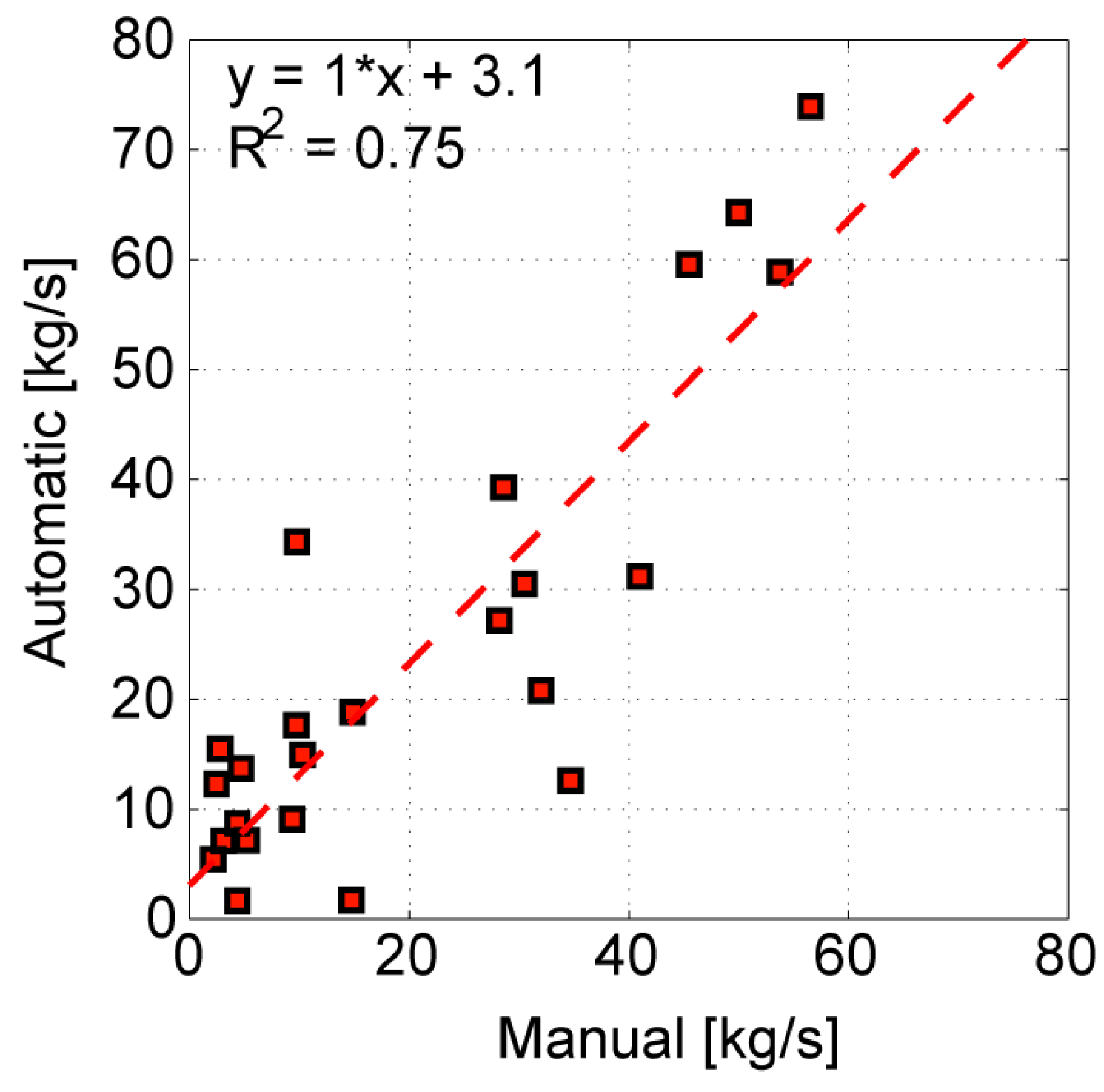
2.3.5. Validation of the Automatic Method

Validity of the automatically processed SO₂ fluxes was tested for a comparison with SO₂ fluxes manually obtained using the Vulcamera software [33] (Figure 6). In particular, this was conducted for some selected days of acquisition characterized by a good weather condition and by clear and well-visible volcanic plume. The manual Vulcamera procedure involves calibrating images by individuation of a clear sky portion unaffected by degassing. Then, SO₂ fluxes were calculated over an integration profile roughly perpendicular to wind direction, using plume speeds obtained from cross-correlation between consecutive frames along the selected profile [33].

Comparison between manually and automatically calculated fluxes (Figure 6) demonstrated a correlation coefficient (R²) of ~0.75, with a best-fit regression line showing a ~1 proportionality factor. The main source of errors was associated with the algorithm for the automatic selection of the background sky area within an image, in particular during highly variable cloud conditions and strong winds. In such cases, background sky detection within images might not be optimal and may then result in a main underestimation of the real SO₂ column densities, as shown by the position of outliers (Figure 6). Overall, this comparison validated the use of the automatic SO₂ flux determination procedure, which paves the way to its full exploitation in real-time volcano monitoring, as already started on the Stromboli volcano (Italy) [32].

3. Results: Application of the Automatic Real Time Algorithm: the Etna 2016 Case

Etna is one of the volcanoes worldwide with the longest and most continuous SO₂ flux record. SO₂ flux measurements have become fundamental in volcano monitoring to define the rates of magma ascent and degassing within the shallow (<3 km) plumbing system. SO₂ fluxes have been measured on Etna since the 1970s using the COSPEC (Correlation Spectrometer) [49,61,62,63,64] and, more recently, a network of Differential Optical absorption spectrometers (FLAME [65,66]). In view of its recurrent activity and robust past SO₂ flux record, Mt. Etna is an ideal test site for validating our automatic processing method.

We reported below on the SO₂ data automatically acquired and processed during 2016, which is a period characterized by substantial temporal changes in activity styles, including a phase of reduced degassing in the aftermaths of the December 2015 eruption [30,67]. This was followed by gradual activity escalation culminating into the May 2016 eruptive phase, and in a new vent opening episode on the eastern VOR crater rim in August [68,69,70].

Our aim was to test if different SO₂ degassing regimes, related to such diverse activity styles, could be resolved and characterized in automatic (and in nearly real-time) using our permanent SO₂ camera system.

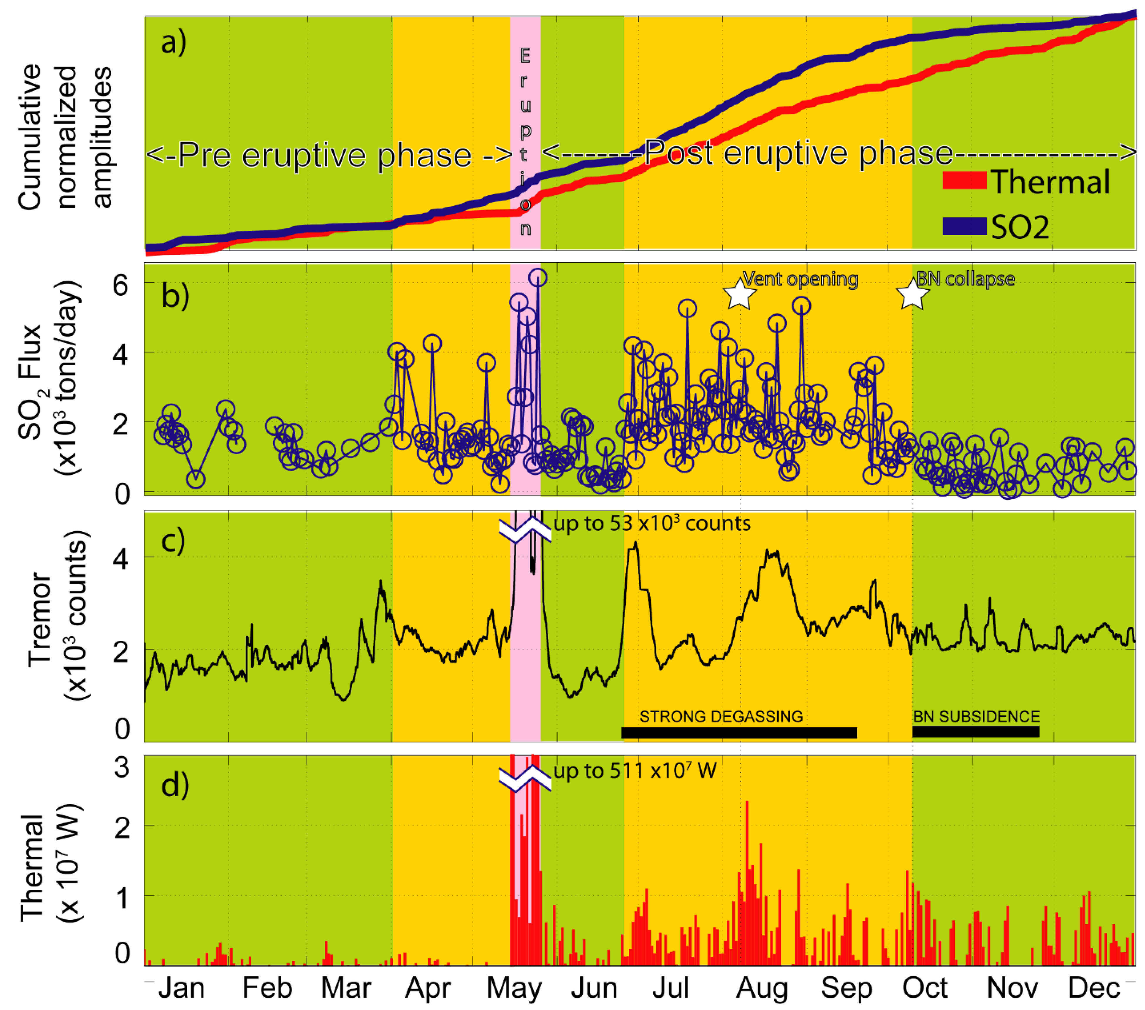
3.1. Etna’s Activity in 2016, SO₂ Flux Records, and Comparison with Seismic, Thermal Dataset, and Field Observations

The SO₂ flux time-series of 2016, which were generated by using the automated processing algorithm proposed in this study, is illustrated in Figure 7. The figure highlights that the significant variability in volcanic activity style in 2016 reflected a highly dynamic SO₂ flux behavior (Figure 7). As illustrated in Figure 7, our 2016 temporal record shows daily averaged SO₂ fluxes ranging between a few hundred to ~6000 tons per day (t/d). The associated standard deviations range from 100 to 4000 t/d. To assist interpretation of SO₂ flux variations, we also reported seismic tremor and thermal radiance time-series (Figure 7), where the latter is expressed as Volcanic Radiative Power (VRP) [71].

Combined analysis of field observations reported in Reference [56] including thermal, seismic, and SO₂ fluxes time-series allowed us to distinguish three main periods of activity: (1) a pre-eruptive period (January to 16 May 2016), in which volcanic activity remained low (January to March) or gradually resuming (April to 16 May), (2) an eruptive period between 16 May and 25 May, characterized by intense strombolian activity, lava flows, and three short-lived lava fountaining episodes that occurred in a brief time lapse between 18 May and 21 May, (3) a post-eruptive period (26 May to 31 December), that included a brief period of reduced activity until the end of June, which is followed by gradual (re)intensification of volcanic activity culminating with opening of new, strongly degassing incandescent vent at VOR on 7 August. This strong degassing declined during the subsidence of the Bocca Nuova (BN) crater’s floor that occurred on October 10. These periods are described in more detail in the following sections.

3.1.1. Volcanic Activity from 1 January 2016 to 15 May 2016 (Pre-Eruptive Period)

Volcanic activity from January to March 2016 was mainly characterized by sporadic ash emissions from the NSEC, and by passive degassing mainly from NEC. The daily average of SO₂ fluxes fluctuated at low levels around ~1500 tons/day. The seismic tremor was stable at around low levels for Etna, and thermal activity occurred at reduced levels (<4 MW) (Figure 7).

Starting from the beginning of April, SO₂ emissions gradually intensified and reached daily averaged fluxes of ~2000 t/d, and seismic tremor fluctuated within a subtle increasing trend. No significant thermal anomaly was still observed (Figure 7), and no significant volcanic activity change was reported from field observations, with NEC still passively degassing and NSEC producing a little more frequent ash emissions with occasional blocks ejected.

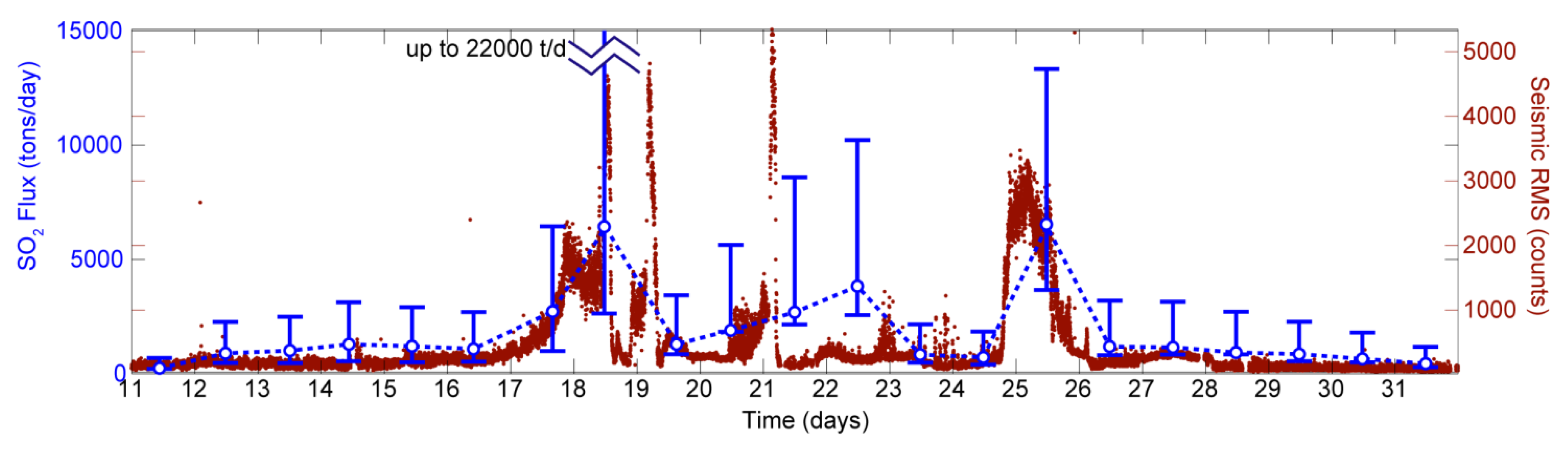
3.1.2. The May Eruptive Period (16–25 May)

In the early morning of 16 May, strombolian activity resumed at NSEC and NEC, and became very strong at the latter crater on 17 May (also reported by References [68,69,70]). On 18 May at 10:50 UTC, a lava fountain started at VOR, which had been quiescent since 3 December, 2015. This event marked the beginning of a paroxysmal sequence, lasting until 25 May. The sequence included two additional short-lived lava fountaining episodes at VOR, on 19 May and 21 May, and ended with an intense strombolian and lava flow activity that lasted several hours (Figure 7 and Figure 8). Lava effusion accompanied all the strongest explosive episodes, issuing from both fissures on the summit cone and overflow from its crater rim. In particular, overflowing from the BN crater rim formed a large lava field that extended downslope up to 3 km. The cumulative volume of lava flows and pyroclastic fall deposits was preliminary estimated at 7 to 10 Mm³ [56], which is similar to what erupted during the December 2015 paroxysmal sequence [30]. Lastly, the summit crater’s area was affected by intense deformation with fracturing, subsidence, and a formation of a ~1 km-long and nearly NS oriented graben-like structure (Figure 1b).

Thermal radiance and the seismic tremor showed coherent increases of three and two order of magnitude, respectively (Figure 7 and Figure 8). The three lava fountains were clearly marked by short-lived peaks in seismic tremor amplitude on 18, 19, and 21 May (Figure 8). The 24–25 May episode of intense strombolian activity/lava fountaining was associated with a wider, longer-lived phase of seismic tremor increase (Figure 8).

The daily averaged SO₂ fluxes increased up to 6000 tons/day (Figure 7), pointing to heightened degassing, nearly tripled with respect to the pre-eruptive phase. A detail of the SO₂ fluxes recorded during the May 2016 paroxysmal sequence is illustrated in Figure 8, where alternation of eruptive and repose periods were evident in the degassing record, with peaks in daily averaged SO₂ flux in three (18, 21 and 25 May) out of four days of paroxysmal activity.

It is also worth noting that only the first (18 May) lava fountaining episode occurred during the UV-camera acquisition temporal interval (see Section 3.2). The high daily averaged SO₂ fluxes obtained on this specific day (Figure 8), thus, reflected the “explosive” SO₂ contribution during the paroxysmal event. In contrast, the SO₂ flux peaks on 22 and 25 May could not be explained by syn-explosive SO₂ release (the lava fountains occurred outside the camera acquisition hours), but rather reflected heightened passive degassing, and/or milder (strombolian) explosive activity, prior to/after the paroxysmal episode itself.

3.1.3. Volcanic Activity after the Eruptive Phase (26 May–31 Dec)

Reduced degassing emissions (<2000 t/d) were measured after the eruptive phase, from May 26^th until the end of June (~1 month), which they could interpret as the aftermath of voluminous gas/magma release during the previous December 2015 [30,39,67,72] and May 2016 eruptive sequences. Field observations indicated that the summit craters were weakly fuming and occluded by lavas and pyroclasts. A progressive subsidence occurred on the VOR crater’s floor, where lunar cracks formed on the crust of the spatter deposits that had filled the crater. Since early July, intensification of SO₂ degassing (average daily fluxes increased from ~900 to ~3000 tons/day, Figure 7) was accompanied by crack widening near the eastern VOR’s crater rim, along the graben-like structure (Figure 1), which culminated, on 7 August, by opening a new 20-m large pit vent, characterized by vigorous high temperature degassing and glowing at night (Figure 1c) [69]. Consistently, thermal activity, as detected by MIROVA, increased in early July from <5 to ~10 MW, which was also reported by Reference [69], and a notable increase was also observed on the seismic tremor (Figure 7). However, repeated inspections on the summit area did not reveal any evidence of explosive activity such as fallout material deposited around the pit vent (as reported in Reference [56]).

From 10 October, after a small explosion, a large subsidence of the BN north-western inner floor was observed. This affected lavas and pyroclastic materials that had filled the central craters during the 2015–2016 paroxysmal sequences. This inner crater subsidence, characterized by episodic collapses, was nicely paralleled by declining SO₂ fluxes down to low values (~1000 tons/day on average). RMS seismic amplitude and thermal radiance slightly decreased as well.

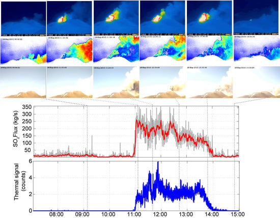
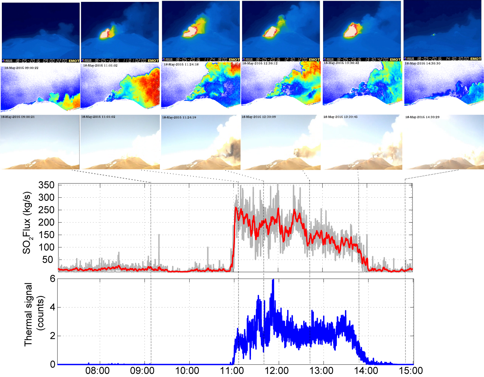
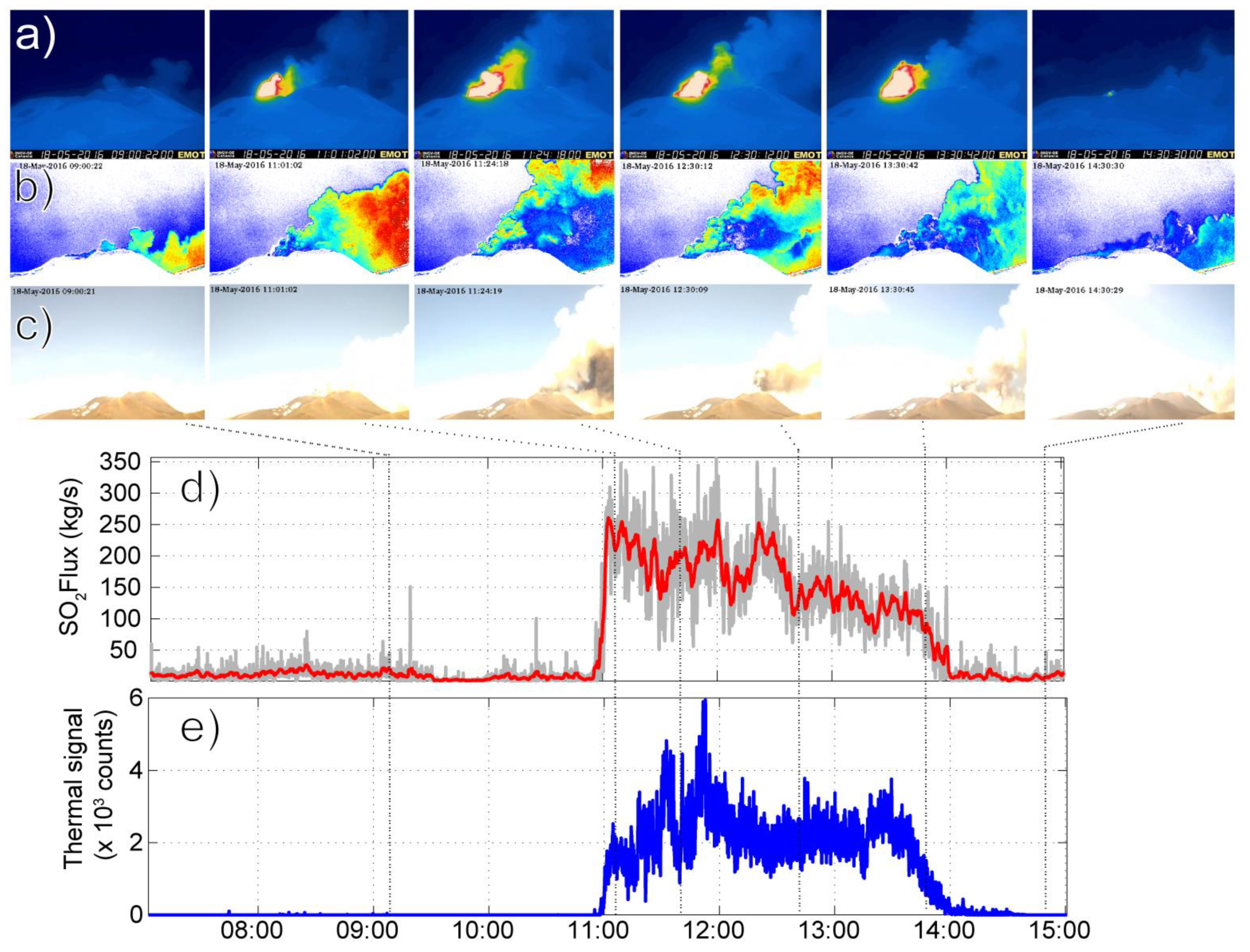
3.2. Syn-Explosive SO₂ Emissions during the Lava Fountaining Event

The 18 May lava fountaining event, entirely captured by the SO₂ camera (Figure 9), allowed us to explore to what extent SO₂ cameras could resolve the degassing dynamics associated with a lava fountaining event. Lava fountains are of special concern at Etna since the volcanic ash they inject into the atmosphere is a potential threat to aviation and population living in the surroundings [73]. These events, while very well monitored and understood [34,36,37,38,39,40,41,42,50,74,75,76,77], are poorly characterized in terms of their associated gas emission rates and volumes. Our 18 May results (Figure 9), therefore, represent one of the first syn-explosive gas records on the volcano [28,30].

Onset of the lava fountain at 10:57 UTC, as constrained by co-acquired images of the INGV-OE thermal and visual cameras (Figure 9), was clearly detected as a visible SO₂ flux increase up to ~260 kg/s (22000 t/d), relative to a pre-eruptive level of ~12 kg/s (~1000 t/d). In the following hour, while activity escalated to peak at ~ 11.30–12.00 (see thermal records), a fluctuating and irregular SO₂ flux trend is registered (Figure 9). Co-acquired thermal and visual images (see panels in Figure 9), clearly indicated that negative peaks in the SO₂ flux time-series were systematically associated with the presence of ash. The latter severely impacts SO₂ detection via UV cameras [21], particularly in near-vent measurements where plumes can be very ash-rich and, thus, optically opaque. Thermal and visual observations showed that ash caused high-frequency fluctuations (short-lived negative peaks) in the SO₂ flux record particularly during the paroxysm climax (~11.30–12.00), but also prior to the lava fountain onset, e.g., after 09.00 when the visual camera captured the first ash emission with no thermal anomaly yet detected (Figure 9).

4. Discussion

Our results demonstrated the ability of the novel automatic processing routine to capture fluctuations in the SO₂ regime, which responded to changes in Etna’s activity style (Figure 7). The automatically processed SO₂ data were consistent with those manually obtained (Figure 6). However, requiring no operator time and being obtained/delivered in nearly real-time, they represented a clear advantage for monitoring purposes.

Our 2016 UV camera-based dataset also provided novel insights into the relationship between rates/modes of SO₂ release and eruptive/degassing styles. These latter were quite diverse in 2016 since they ranged from non-eruptive quiescent degassing to intense paroxysmal activity in May. Nicely, our automatically processed SO₂ fluxes peaked during heightened activity (Figure 7 and Figure 8) during the May 2016 eruptive sequence, and during the July-August degassing unrest that led to opening of the VOR incandescent vent on 7 August.

One important observation is the mild but significant SO₂ flux increase in April 2016, as demonstrated by a clear change in the slope of the cumulative SO₂ mass (see orange-coloured area in Figure 7a). The SO₂ flux increase started more than one month before onset of the May eruptive sequence, which is a period when the seismic tremor was at average levels and no significant thermal anomaly was detected (Figure 7). We interpreted these escalating SO₂ fluxes as reflecting the slow but systematic increase in the magma supply rate to the shallow (<3 km [78]) Etna’s magma feeding system that triggered the May 2016 paroxysmal sequence [68]. However, while the relatively subtle changes in SO₂ passive degassing in April 2016 may have represented a precursory sign for the imminent (May 2016) eruption, we still noticed that a similar SO₂ increase was observed from July to September 2016 (orange-coloured sub-interval in Figure 7a). This did not culminate into an eruption yet (if not for the opening of the 7 August summit vent). Thus, the volcano’s feedback to increased shallow magma emplacement (as indicated by increasing SO₂ fluxes) may be different from time to time, perhaps in response to distinct stress regimes prevailing on the upper part of the edifice, and/or temporally varying feedbacks between magma ascent and rates of gravitational spreading of the mobile eastern flank [79,80].

We also characterized SO₂ emissions associated with a lava fountaining event at a high spatial and temporal resolution [28,30]. Even though ash is a serious issue for ground-based SO₂ remote sensing during explosive eruptions, we still noted that the entirety of 18 May eruptive episode was well marked by elevated SO₂ fluxes well above background emissions in the pre-event and post-event phases. In fact, SO₂ emissions manifestly dropped down at only 14:00 UTC, when declining thermal emissions consistently marked lava fountaining termination. From such, we found it useful to tentatively estimate the cumulative SO₂ mass released by the 18 May lava-fountain, by integrating the signal over the eruption duration. We obtained a total SO₂ mass released in the event of ~1700 tons, and an average flux of 158 kg/s (13,600 t/d) for a total duration of ~3 h. We caution this inferred mass corresponds to a lower range estimate, due to the presence of volcanic ash that severely depressed the measured SO₂ signal during the eruption climax.

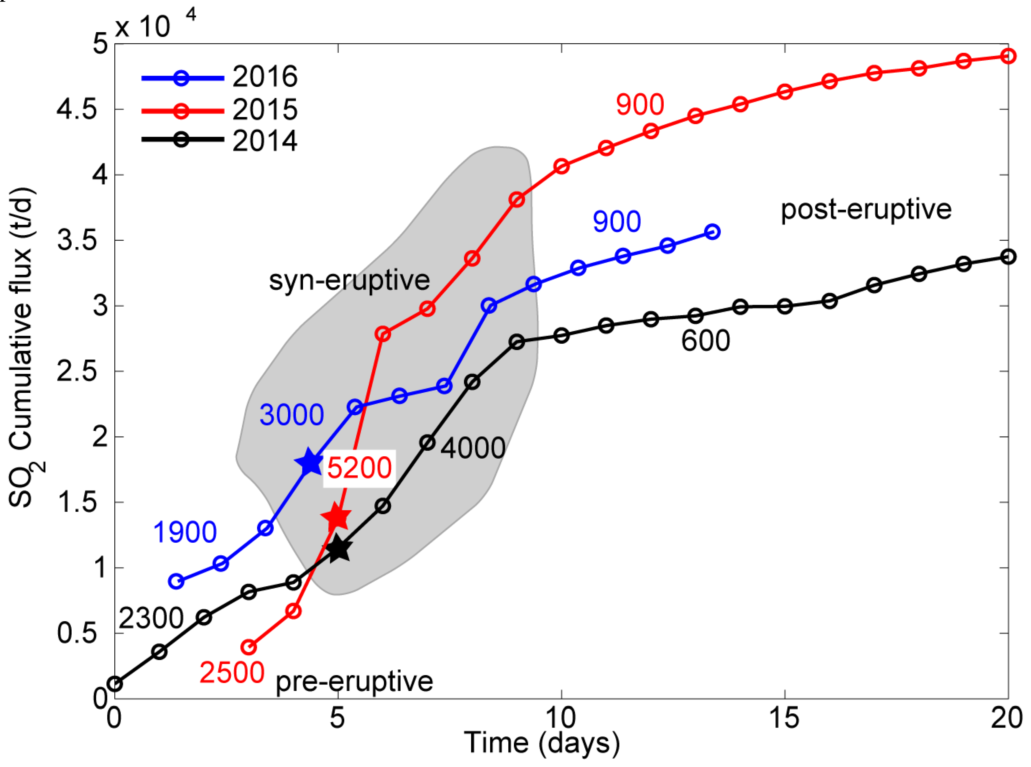
SO₂ Fluxes during the May 2016 Eruptive Sequence: Comparison with 2014–2015 Results

It is well established that SO₂ fluxes are directly linked to the rate of magma ascent and degassing [78]. Thus, temporal variations in SO₂ fluxes do reflect changes in magma feeding to the volcano’s shallow plumbing system, and, as such, may help track transition in activity style, from quiet passive degassing to eruptive periods [81]. On Etna, we now have 3 years of UV camera observations available ([28,30], this study), during which transition from quiescence to eruption has frequently been observed. We, thus, examined our dataset in the attempt to tentatively identify any possible systematic SO₂ flux threshold/trend corresponding to such an activity switch.

For this purpose, in Figure 10, we compared the cumulative SO₂ flux trends (time-normalized) for three different periods encompassing three eruptive paroxysmal episodes, which occurred in August 2014, December 2015, and May 2016, respectively. For each of three events, we calculated the averaged SO₂ fluxes (corresponding to the slopes of the cumulative curve) in the periods before, during, and after eruption, and we found significant similarities between the three events. In each of the three 2014–2016 events, the pre-eruptive fluxes fell in a relatively narrow range, between 1900 and 2500 t/d. The syn-eruptive (during the paroxysmal sequence) fluxes were typically higher, and spanned between 3000 and 5200 t/d (Figure 10), and were the highest during the December 2015 paroxysmal sequence that was consistently the most energetic in the past few years [67]. Lastly, each of the three post-paroxysmal phases was characterized by reduced SO₂ emissions, ranging between 600 and 900 t/d, which impliesa reduced magma supply and degassing of a volatile depleted (residual) magma after each eruptive episode. These ranges were fully in agreement with those indicated by Reference [49] and by the analysis of a 13-year-long dataset.

Our preliminary results are suggestive of the existence of a systematic pattern in SO₂ emissions that, if confirmed, would imply a recurrent degassing process/mechanism prior to, during, and after the Etna’s eruptive periods. Clearly, additional data are required to corroborate this initial hypothesis.

5. Conclusions

SO₂ imaging at Mt Etna during 2016 revealed different styles of gas emissions, which reflected changes in volcanic activity, from quietly passive degassing to eruptive activity (lava fountaining, intense strombolian activity, and lava flowing).

To real-time characterize and monitor this very dynamic activity period, we designed a novel routine to automatically calculate SO₂ fluxes including computer-based detection of image quality, and calculation of plume speed time-series using computer vision libraries. This automatic processing routine allowed us to obtain real-time information on volcano degassing dynamics at high spatial and temporal resolution, which results in a further step in instrumental volcanic gas monitoring. We validated the methodology through a comparison with manually processed results and integration with independent thermal and seismic observations. All these independent datasets showed coherent temporal variations that validated the use of UV cameras for detecting subtle changes in volcanic and degassing activity. Our novel method, thus, promises a step ahead in instrumental volcanic gas monitoring.

Our automatically derived SO₂ flux time-series were used to constrain degassing regimes on Mt. Etna in 2016. We have shown that our automatically processed SO₂ fluxes peaked during heightened activity, such as during the May 2016 eruptive sequence, and during a phase of elevated degassing in July–August 2016, which culminated with the opening of a new summit incandescent vent. The May 2016 sequence was preceded by a circa one-month-long phase of a mild but detectable SO₂ flux increase, and was followed by an abrupt drop in degassing. Comparison between our SO₂ flux time-series in May 2016 and those associated with two other eruptive paroxysmal sequences (occurred in 2014 and 2015) highlighted strong similarities in SO₂ flux dynamics, which implies the possible existence of thresholds that distinguish between degassing regimes, prior to, during, and after eruptions. Pre-paroxysm SO₂ fluxes were found to have consistent values (of ~2000 t/d) during the three episodes. Similarly, the highest SO₂ fluxes (from 3000 t/d up to 5200 t/d on a daily average basis) were identified during the three eruptive sequences, while post-eruptive were systematically characterized by reduced degassing (<1000 t/d). This result, if confirmed by future observations, may bring implications for identifying switches in volcanic activity regime. We believe this methodology can be successfully exported on other open-vent active volcanoes, after a relatively brief period of calibration.

We also tested the ability of UV camera records to characterizing SO₂ emissions during a lava fountain episode. This is, to the best of our knowledge, one of the first SO₂ camera record at high spatial and temporal resolution of an ongoing lava fountaining [28,30]. We have reported on high levels of degassing during the lava fountain (of up to 260 kg/s), from which we assessed a lower limit (due to the ash presence within the plume) for the cumulative SO₂ mass of ~1700 tons emitted during a lava fountain episode.

References

1. Oppenheimer, C.; Fischer, T.P.; Scaillet, B. Volcanic Degassing: Process and Impact. In Treatise on Geochemistry, The Crust; Holland, H.D., Turekian, K.K., Eds.; Elsevier: Amsterdam, The Netherlands, 2014; Volume 4, pp. 111–179. [Google Scholar]
2. Fischer, T.P.; Chiodini, G. Volcanic, Magmatic and Hydrothermal Gas Discharges. In Encyclopaedia of Volcanoes, 2nd ed.; Academic Press: Cambridge, MA, USA, 2015; pp. 779–797. [Google Scholar] [CrossRef]
3. Aiuppa, A. Volcanic Gas Monitoring. In Volcanism and Global Environmental Change; Schmidt, A., Fristad, K.E., Elkins-Tanton, L.T., Eds.; Cambridge University Press: Cambridge, UK, 2015; pp. 81–96. [Google Scholar]
4. Wallace, P.J.; Kamenetsky, V.S.; Cervantes, P. Melt inclusion CO2 contents, pressures of olivine crystallization, and the problem of shrinkage bubbles. Am. Mineral. 2015, 100, 787–794. [Google Scholar] [CrossRef]
5. Saccorotti, G.; Iguchi, M.; Aiuppa, A. In situ Volcano Monitoring: Present and Future. In Volcanic Hazards, Risks, and Disasters; Shroder, J.F., Papale, P., Eds.; Elsevier: Amsterdam, The Netherlands, 2015; pp. 169–202. [Google Scholar]
6. Galle, B.; Oppenheimer, C.; Geyer, A.; McGonigle, A.J.S.; Edmonds, M.; Horrocks, L.A. A miniaturized ultraviolet spectrometer for remote sensing of SO2 fluxes: A new tool for volcano surveillance. J. Volcanol. Geotherm. Res. 2003, 119, 241–254. [Google Scholar] [CrossRef]
7. Galle, B.; Johansson, M.; Rivera, C.; Zhang, Y.; Kihlman, M.; Kern, C.; Lehmann, T.; Platt, U.; Arellano, S.; Hidalgo, S. Network for Observation of Volcanic and Atmospheric Change (NOVAC): A global network for volcanic gas monitoring: Network layout and instrument description. J. Geophys. Res. 2010, 115, D05304. [Google Scholar] [CrossRef]
8. Christopher, T.; Edmonds, M.; Humphreys, M.C.S.; Herd, R.A. Volcanic gas emissions from Soufrière Hills Volcano, Montserrat 1995–2009, with implications for mafic magma supply and degassing. Geophys. Res. Lett. 2010, 37, L00E04. [Google Scholar] [CrossRef]
9. Mori, T.; Shinohara, H.; Kazahaya, K.; Hirabayashi, K.; Matsushima, T.; Mori, T.; Ohwada, M.; Odai, M.; Iino, H.; Miyashita, M. Time-averaged SO2 fluxes of subduction-zone volcanoes: Example of a 32-year exhaustive survey for Japanese volcanoes. J. Geophys. Res. Atmos. 2013, 118, 8662–8674. [Google Scholar] [CrossRef]
10. Hidalgo, S.; Battaglia, J.; Arellano, S.; Steele, A.; Bernard, B.; Bourquin, J.; Galle, B.; Arrais, S.; Vásconez, F. SO2 degassing at Tungurahua volcano (Ecuador) between 2007 and 2013: Transition from continuous to episodic activity. J. Volcanol. Geothem. Res. 2015, 298, 1–14. [Google Scholar] [CrossRef]
11. McGonigle, A.J.S.; Hilton, D.R.; Fischer, T.P.; Oppenheimer, C. Plume velocity determination for volcanic SO2 flux measurements. Geophys. Res. Lett. 2005, 32. [Google Scholar] [CrossRef]
12. Mori, T.; Burton, M.R. The SO2 camera: A simple, fast and cheap method for ground-based imaging of SO2 in volcanic plumes. Geophys. Res. Lett. 2006, 33, L24804. [Google Scholar] [CrossRef]
13. Burton, M.R.; Prata, F.; Platt, U. Volcanological applications of SO2 cameras. J. Volcanol. Geothem. Res. 2015, 300, 2–6. [Google Scholar] [CrossRef]
14. Burton, M.R.; Salerno, G.; D’Auria, L.; Caltabiano, T.; Murè, F.; Maugeri, R. SO2 flux monitoring at Stromboli with the new permanent INGV SO2 camera system: A comparison with the FLAME network and seismological data. J. Volcanol. Geothem. Res. 2015, 300, 95–102. [Google Scholar] [CrossRef]
15. McGonigle, A.J.S.; Pering, T.D.; Wilkes, T.C.; Tamburello, G.; D’Aleo, R.; Bitetto, M.; Aiuppa, A.; Willmott, J.R. Ultraviolet Imaging of Volcanic Plumes: A New Paradigm in Volcanology. Geosciences 2017, 7, 68. [Google Scholar] [CrossRef]
16. Dalton, M.P.; Waite, G.P.; Watson, I.M.; Nadeau, P.A. Multiparameter quantification of gas release during weak Strombolian eruptions at Pacaya Volcano, Guatemala. Geophys. Res. Lett. 2010, 37. [Google Scholar] [CrossRef]
17. Holland, P.A.S.; Watson, M.I.; Phillips, J.C.; Caricchi, L.; Dalton, M.P. Degassing processes during lava dome growth: Insights from Santiaguito lava dome, Guatemala. J. Volcanol. Geotherm. Res. 2011, 202, 153–166. [Google Scholar] [CrossRef]
18. Kazahaya, R.; Mori, T.; Takeo, M.; Ohminato, T.; Urabe, T.; Maeda, Y. Relation between single very long period pulses and volcanic gas emissions at Mt. Asama, Japan. Geophys. Res. Lett. 2011, 38. [Google Scholar] [CrossRef]
19. Kazahaya, R.; Shinohara, H.; Mori, T.; Iguchi, M.; Yokoo, A. Pre-eruptive inflation caused by gas accumulation: Insight from detailed gas flux variation at Sakurajima volcano, Japan. Geophys. Res. Lett. 2016, 43, 21. [Google Scholar] [CrossRef]
20. Nadeau, P.A.; Jose, L.P.; Waite, G.P. Linking volcanic tremor, degassing, and eruption dynamics via SO2 imaging. Geophys. Res. Lett. 2011, 38, L01304. [Google Scholar] [CrossRef]
21. Tamburello, G.; Aiuppa, A.; Kantzas, E.P.; McGonigle, A.J.S.; Ripepe, M. Passive vs. active degassing modes at an open-vent volcano (Stromboli, Italy). Earth Planet. Sci. Lett. 2012, 359–360, 106–116. [Google Scholar] [CrossRef]
22. Tamburello, G.; Aiuppa, A.; McGonigle, A.J.S.; Allard, P.; Cannata, A.; Giudice, G.; Kantzas, E.P.; Pering, T.D. Periodic volcanic degassing behavior: The Mount Etna example. Geophys. Res. Lett. 2013, 40, 4818–4822. [Google Scholar] [CrossRef]
23. Waite, G.P.; Nadeau, P.A.; Lyons, J.J. Variability in eruption style and associated very long period events at Fuego volcano, Guatemala. J. Geophys. Res. Solid Earth 2013, 118, 1526–1533. [Google Scholar] [CrossRef]
24. Pering, T.D.; Tamburello, G.; Mc Gonigle, A.J.S.; Aiuppa, A.; Cannata, A.; Giudice, G.; Patanè, D. High time resolution fluctuations in volcanic carbon dioxide degassing from Mount Etna. J. Volcanol. Geotherm. Res. 2014, 270, 115–121. [Google Scholar] [CrossRef]
25. Pering, T.D.; Tamburello, G.; McGonigle, A.J.S.; Aiuppa, A.; James, M.R.; Lane, S.J.; Sciotto, M.; Cannata, A.; Patanè, D. Dynamics of mild strombolian activity on Mt. Etna. J. Volcanol. Geothem. Res. 2015, 300, 103–111. [Google Scholar] [CrossRef]
26. Pering, T.D.; McGonigle, A.J.S.; James, M.R.; Tamburello, G.; Aiuppa, A.; Delle Donne, D.; Ripepe, M. Conduit dynamics and post explosion degassing on Stromboli: A combined UV camera and numerical modeling treatment. Geophys. Res. Lett. 2016, 43, 5009–5016. [Google Scholar] [CrossRef] [PubMed]
27. Nadeau, P.A.; Werner, C.A.; Waite, G.P.; Carn, S.A.; Brewer, I.D.; Elias, T.; Sutton, A.J.; Kern, C. Using SO2 camera imagery and seismicity to examine degassing and gas accumulation at Kīlauea Volcano, May 2010. J. Volcanol. Geotherm. Res. 2015, 300, 70–80. [Google Scholar] [CrossRef]
28. D’Aleo, R.; Bitetto, M.; Delle Donne, D.; Tamburello, G.; Battaglia, A.; Coltelli, M.; Patanè, D.; Prestifilippo, M.; Sciotto, M.; Aiuppa, A. Spatially resolved SO2 flux emissions from Mt Etna. Geophys. Res. Lett. 2016, 43. [Google Scholar] [CrossRef] [PubMed]
29. Wilkes, T.C.; Pering, T.D.; McGonigle, A.J.S.; Tamburello, G.; Willmott, J.R. A Low-Cost Smartphone Sensor-Based UV Camera for Volcanic SO2 Emission Measurements. Remote Sens. 2017, 9, 27. [Google Scholar] [CrossRef]
30. D’Aleo, R.; Bitetto, M.; Delle Donne, D.; Coltelli, M.; Coppola, D.; Mc Cormick Kilbride, B.; Pecora, E.; Ripepe, M.; Salem, L.; Tamburello, G.; et al. Understanding the SO2 Degassing Budget of Mt Etna’s Paroxysms: First Clues from the December 2015 Sequence. Front. Earth Sci. 2019, 6, 239. [Google Scholar] [CrossRef]
31. Kern, C.; Sutton, J.; Elias, T.; Lee, L.; Kamibayashi, K.; Antolik, L.; Werner, C. An automated SO2 camera system for continuous, real-time monitoring of gas emissions from Kīlauea Volcano’s summit Overlook Crater. J. Volcanol. Geothem. Res. 2015, 300, 81–94. [Google Scholar] [CrossRef]
32. Delle Donne, D.; Tamburello, G.; Aiuppa, A.; Bitetto, M.; Lacanna, G.; D’Aleo, R.; Ripepe, M. Exploring the explosive-effusive transition using permanent ultraviolet cameras. J. Geophys. Res. Solid Earth 2017, 4377–4394. [Google Scholar] [CrossRef]
33. Tamburello, G.; Kantzas, E.P.; McGonigle, A.J.S.; Aiuppa, A. Vulcamera: A program for measuring volcanic SO2 using UV cameras. Ann. Geophys. 2011, 54, 2. [Google Scholar]
34. Alparone, S.; Andronico, D.; Lodato, L.; Sgroi, T. Relationship between tremor and volcanic activity during the Southeast Crater eruption on Mount Etna in early 2000. J. Geophys. Res. 2003, 108, 2241. [Google Scholar] [CrossRef]
35. Vergniolle, S.; Ripepe, M. From Strombolian explosions to fire fountains at Etna Volcano (Italy): What do we learn from acoustic measurements? Geol. Soc. Lond. Spec. Publ. 2008, 307, 103–124. [Google Scholar] [CrossRef]
36. Patanè, D.; Aiuppa, A.; Aloisi, M.; Behncke, B.; Cannata, A.; Coltelli, M.; Di Grazia, G.; Gambino, S.; Gurrieri, S.; Mattia, M. Insights into magma and fluid transfer at Mount Etna by a multiparametric approach: A model of the events leading to the 2011 eruptive cycle. J. Geophys. Res. Solid Earth 2013, 118, 3519–3539. [Google Scholar] [CrossRef]
37. Bonaccorso, A.; Calvari, S.; Currenti, G. From source to surface: Dynamics of Etna’s lava fountains investigated by continuous strain, magnetic, ground and satellite thermal data. Bull. Volcanol. 2013, 75. [Google Scholar] [CrossRef]
38. Bonaccorso, A.; Calvari, S.; Linde, A.; Sacks, S. Eruptive processes leading to the most explosive lava fountain at Etna volcano: The 23 November 2013 episode. Geophys. Res. Lett. 2014, 41, 4912–4919. [Google Scholar] [CrossRef]
39. Bonaccorso, A.; Calvari, S. A new approach to investigate an eruptive paroxysmal sequence using camera and strainmeter networks: Lessons from the 3–5 December 2015 activity at Etna volcano. Earth Planet. Sci. Lett. 2017, 475, 231–241. [Google Scholar] [CrossRef]
40. Spampinato, L.; Sciotto, M.; Cannata, A.; Cannavò, F.; La Spina, A.; Palano, M.; Salerno, G.; Privitera, E.; Caltabiano, T. Multiparametric study of the February–April 2013 paroxysmal phase of Mt. Etna New South-East crater. Geochem. Geophys. Geosyst. 2015, 16, 1932–1949. [Google Scholar] [CrossRef]
41. Gambino, S.; Cannata, A.; Cannavò, F.; La Spina, A.; Palano, M.; Sciotto, M.; Spampinato, L.; Barberi, G. The unusual 28 December 2014 dike-fed paroxysm at Mount Etna: Timing and mechanism from a multidisciplinary perspective. J. Geophys. Res. Solid Earth 2016, 121, 2037–2053. [Google Scholar] [CrossRef]
42. Ripepe, M.; Marchetti, E.; Delle Donne, D.; Genco, R.; Innocenti, L.; Lacanna, G.; Valade, S. Infrasonic Early Warning System for Explosive Eruptions. J. Geophys. Res. Solid Earth 2018, 123, 9570–9585. [Google Scholar] [CrossRef]
43. Coppola, D.; Laiolo, M.; Cigolini, C.; Delle Donne, D.; Ripepe, M. Enhanced volcanic hot-spot detection using MODIS IR data: Results from the MIROVA system. Geol. Soc. Lond. Spec. Publ. 2015, 426, SP426. [Google Scholar] [CrossRef]
44. Andò, B.; Pecora, E. An advanced video-based system for monitoring active volcanoes. Comput. Geosci. 2006, 32, 85–91. [Google Scholar] [CrossRef]
45. Kantzas, E.P.; McGonigle, A.J.S.; Tamburello, G.; Aiuppa, A.; Bryant, R.G. Protocols for UV camera volcanic SO2 measurements. J. Volcanol. Geothem. Res. 2010, 194, 55–60. [Google Scholar] [CrossRef]
46. Kern, C.; Deutschmann, T.; Vogel, L.; Wöhrbach, M.; Wagner, T.; Platt, U. Radiative transfer corrections for accurate spectroscopic measurements of volcanic gas emissions. Bull. Volcanol. 2010, 72, 233–247. [Google Scholar] [CrossRef]
47. McGonigle, A.J.S. Measurement of volcanic SO2 fluxes with differential optical absorption spectroscopy. J. Volcanol. Geoth. Res. 2007, 162, 111–122. [Google Scholar] [CrossRef]
48. Vandaele, A.C.; Simon, P.C.; Guilmot, J.M.; Carleer, M.; Colin, R. SO2 absorption cross section measurement in the UV using a Fourier transform spectrometer. J. Geophys. Res. 1994, 99, 25–599. [Google Scholar] [CrossRef]
49. Caltabiano, T.; Burton, M.; Giammanco, S.; Allard, P.; Bruno, N.; Murè, F.; Romano, R. Volcanic Gas Emissions from the Summit Craters and Flanks of Mt. Etna, 1987–2000. In Mt. Etna: Volcano Laboratory; Bonaccorso, A., Calvari, S., Coltelli, M., Del Negro, C., Falsaperla, S., Eds.; Geophysical Monograph Series; American Geophysical Union: Washington, DC, USA, 2004; Volume 143, pp. 111–128. [Google Scholar]
50. Ulivieri, G.; Ripepe, M.; Marchetti, E. Infrasound reveals transition to oscillatory discharge regime during lava fountaining: Implication for early warning. Geophys. Res. Lett. 2013, 40, 3008–3013. [Google Scholar] [CrossRef]
51. Zuccarello, L.; Burton, M.R.; Saccorotti, G.; Bean, C.J.; Patanè, D. The coupling between very long period seismic events, volcanic tremor, and degassing rates at Mount Etna volcano. J. Geophys. Res. Solid Earth 2013, 118, 4910–4921. [Google Scholar] [CrossRef]
52. Salerno, G.G.; Burton, M.R.; Di Grazia, G.; Caltabiano, T.; Oppenheimer, C. Coupling Between Magmatic Degassing and Volcanic Tremor in Basaltic Volcanism. Front. Earth Sci. 2018, 6, 157. [Google Scholar] [CrossRef]
53. Harris, A.J.L. Thermal Remote Sensing of Active Volcanoes: A User’s Manual; Cambridge University Press: Cambridge, UK, 2013; p. 716. [Google Scholar]
54. Aiuppa, A.; De Moor, J.M.; Arellano, S.; Coppola, D.; Francofonte, V.; Galle, B. Tracking formation of a lava lake from ground and space: Masaya volcano (Nicaragua), 2014–2017. Geochem. Geophys. Geosyst. 2018, 19, 496–515. [Google Scholar] [CrossRef]
55. Kern, C. Spectroscopic Measurements of Volcanic Gas Emissions in the Ultra-Violet Wavelength Region. Ph.D. Thesis, University of Heidelberg, Heidelberg, Germany, 2009. [Google Scholar]
56. INGV—Osservatorio Etneo. 2016. Available online: http://www.ct.ingv.it/en/rapporti/multidisciplinari.html (accessed on 26 February 2019).
57. Bluth, G.S.J.; Shannon, J.M.; Watson, I.M.; Prata, A.J.; Realmuto, V.J. Development of an ultra-violet digital camera for volcanic SO2 imaging. J. Volcanol. Geothem. Res. 2007, 161, 47–56. [Google Scholar] [CrossRef]
58. Thomas, H.E.; Prata, A.J. Computer vision for improved estimates of SO2 emission rates and plume dynamics. Int. J. Remote Sens. 2018, 39, 1285–1305. [Google Scholar] [CrossRef]
59. Lucas, B.D.; Kanade, T. An iterative image registration technique with an application to stereo vision. IJCAI 1981, 81, 674–679. [Google Scholar]
60. Bradski, G.; Kaehler, A. Learning OpenCV: Computer Vision with the OpenCV Library; O’Reilly Media: Newton, MA, USA, 2008. [Google Scholar]
61. Moffat, A.J.; Millan, M.M. The applications of optical correlation techniques to the remote sensing of SO2 plumes using sky light. Atmos. Environ. 1971, 5, 677–690. [Google Scholar] [CrossRef]
62. Stoiber, R.E.; Malinconico, L.L., Jr.; Williams, S.N. Use of the Correlation Spectrometer at Volcanoes. In Forecasting Volcanic Events; Tazieff, H., Sabroux, J.C., Eds.; Elsevier: New York, NY, USA, 1983; pp. 425–444. [Google Scholar]
63. Caltabiano, T.; Romano, R.; Budetta, G. SO2 flux measurements at Mount Etna (Sicily). J. Geophys. Res. 1994, 99, 12809–12819. [Google Scholar] [CrossRef]
64. Bruno, N.; Caltabiano, T.; Romano, R. SO2 emissions at Mt.Etna with particular reference to the period 1993–1995. Bull. Volcanol. 1999, 60, 405–411. [Google Scholar] [CrossRef]
65. Burton, M.R.; Caltabiano, T.; Salerno, G.; Murè, F.; Condarelli, D. Automatic measurements of SO2 flux on Stromboli using a network of scanning ultraviolet spectrometers. Geophys. Res. Abstr. 2004, 6, 03970. [Google Scholar]
66. Salerno, G.G.; Burton, M.R.; Oppenheimer, C.; Caltabiano, T.; Tsanev, V.; Bruno, N. Novel retrieval of volcanic SO2 abundance from ultraviolet spectra. J. Volcanol. Geotherm. Res. 2009, 181, 141–153. [Google Scholar] [CrossRef]
67. Pompilio, M.; Bertagnini, A.; Del Carlo, P.; Di Roberto, A. Magma dynamics within a basaltic conduit revealed by textural and compositional features of erupted ash: the December 2015 Mt. Etna paroxysms. Sci. Rep. 2017, 7, 4805. [Google Scholar] [CrossRef] [PubMed]
68. Cannata, A.; Di Grazia, G.; Giuffrida, M.; Gresta, S. Space Time Evolution of Magma Storage and Transfer at Mt. Etna Volcano (Italy): The 2015–2016 Reawakening of Voragine Crater. Geochem. Geophys. Geosyst. 2018, 19, 471–495. [Google Scholar] [CrossRef]
69. Marchese, F.; Neri, M.; Falconieri, A.; Lacava, T.; Mazzeo, G.; Pergola, N.; Tramutoli, V. The Contribution of Multi-Sensor Infrared Satellite Observations to Monitor Mt. Etna (Italy) Activity during May to August 2016. Remote Sens. 2018, 10, 1948. [Google Scholar] [CrossRef]
70. Edwards, M.J.; Pioli, L.; Andronico, D.; Scollo, S.; Ferrari, F.; Cristaldi, A. Shallow factors controlling the explosivity of basaltic magmas: The 17–25 May 2016 eruption of Etna Volcano (Italy). J. Volcanol. Geothem. Res. 2018, 357, 425–436. [Google Scholar] [CrossRef]
71. Coppola, D.; Piscopo, D.; Laiolo, M.; Cigolini, C.; Delle Donne, D.; Ripepe, M. Radiative heat power at Stromboli volcano during 2000–2011: Twelve years of MODIS observations. J. Volcanol.Geoth. Res. 2012, 215, 48–60. [Google Scholar] [CrossRef]
72. Vulpiani, G.; Ripepe, M.; Valade, S. Mass discharge rate retrieval combining weather radar and thermal camera observations. J. Geophys. Res. Solid Earth 2016, 121, 5679–5695. [Google Scholar] [CrossRef]
73. Scollo, S.; Boselli, A.; Coltelli, M. Monitoring Etna volcanic plumes using a scanning LiDAR. Bull. Volcanol. 2012, 74, 2383–2395. [Google Scholar] [CrossRef]
74. Harris, A.J.L.; Neri, M. Volumetric observations during paroxysmal eruptions at Mount Etna: Pressurized drainage of a shallow chamber or pulsed supply? J. Volcanol. Geothem. Res. 2002, 116, 79–95. [Google Scholar] [CrossRef]
75. Dubosclard, G.; Donnadieu, F.; Allard, P.; Cordesses, R.; Hervier, C.; Coltelli, M.; Privitera, E.; Kornprobst, J. Doppler radar sounding of volcanic eruption dynamics at Mount Etna. Bull. Volcanol. 2004, 66, 443–456. [Google Scholar] [CrossRef]
76. Andronico, D.; Corsaro, R.A. Lava fountains during the episodic eruption of South–East Crater (Mt. Etna), 2000: Insights into magma-gas dynamics within the shallow volcano plumbing system. Bull. Volcanol. 2011, 73, 1165. [Google Scholar] [CrossRef]
77. Calvari, S.; Salerno, G.G.; Spampinato, L.; Gouhier, M.; La Spina, A.; Pecora, E.; Harris, A.J.L.; Labazuy, P.; Biale, E.; Boschi, E. An unloading foam model to constrain Etna’s 11–13 January 2011 lava fountaining episode. J. Geophys. Res. 2011, 116, B11207. [Google Scholar] [CrossRef]
78. Allard, P. Endogenous magma degassing and storage at Mount Etna. Geophys. Res. Lett. 1997, 24, 2219–2222. [Google Scholar] [CrossRef]
79. Bonforte, A.; Guglielmino, F.; Puglisi, G. Interaction between magma intrusion and flank dynamics at Mt. Etna in 2008, imaged by integrated dense GPS and DInSAR data. Geochem. Geophys. Geosyst. 2013, 14, 2818–2835. [Google Scholar] [CrossRef]
80. Bonaccorso, A.; Bonforte, A.; Gambino, S. Twenty-five years of continuous borehole tilt and vertical displacement data at Mount Etna: Insights on long-term volcanic dynamics. Geophys. Res. Lett. 2015, 42, 10222–10229. [Google Scholar] [CrossRef]
81. Oppenheimer, C.; Scaillet, B.; Martin, R.S. Sulfur degassing from volcanoes: Source conditions, surveillance, plume chemistry and earth system impacts. Rev. Mineral. Geochem. 2011, 73, 363–421. [Google Scholar] [CrossRef]
Figure 1. (a) The Montagnola site where the UV camera system was installed (position of ETN seismic station is also indicated). Sites from where pictures (c), (d), and (e) have been taken are shown. Black inset identifies the zoomed area of Figure 1b. (b) Etna summit area (redrawn from Reference [56]) shows the active summit craters (BN: Bocca Nuova; VOR: Voragine; NEC: North-East Crater; SEC: South-East Crater; NSEC: New South East Crater), the 7 August degassing vent, and the graben-like structure discussed in the text. The site where picture f has been taken is also shown. (c) Photo showing the Montagnola site and the summit area. (d) Thermal snapshot from INGV-OE monitoring camera capturing the 18 May lava fountaining episode. (e) Vigorous degassing from the vent opened on 7 August. (f) Picture taken from Reference [56] showing BN crater collapse occurred on 10 October, and marking the end of enhanced degassing activity (see text).
Remotesensing 11 01201 g001
Figure 2. Calculation of the SO2 column densities using the dual camera method with 330 nm (a) and 310 nm (b) optical filters. Absorbance image (c) is obtained using the Lambert-Beer equation after image normalization with respect to background absorbance intensities (black circles in (a) and (b), automatically located). Black circles in (a) and (b) represent the sky areas where absorbance is assumed to be SO2 free (minimum absorbance level). Black rectangles (Ssky Sgrn) in (a) represent the areas used for calculation of the visibility index. The red circle in (c) shows the FOV of co-located UV-scanning spectrometer used to convert un-calibrated absorbance intensities into SO2 column densities.
Remotesensing 11 01201 g002
Figure 3. The image quality calculation method using the correlation coefficient between the 310 nm filter image (a) and the corresponding absorbance image (b). An intensity profile associated with a section (dashed line) crossing the volcanic plume, for both the 310-nm filter and absorbance images, is obtained (c). If these profiles are negatively correlated with a high correlation coefficient (d), then the gas is visible within the plume.
Remotesensing 11 01201 g003
Figure 4. Example of output of the quality indexes sub-routine. The visibility (fog) and correlation indexes fluctuate through time as visibility conditions change (see snapshots on top of the figure). Gas is visible only when the fog index is greater than 4 and the correlation index is less than -0.5.
Remotesensing 11 01201 g004
Figure 5. SO2 density flux calculated in the sub-area encompassing the summit craters. White arrows correspond to gas velocity vectors calculated on high coherence regions of the images. SO2 density flux distributions along the entire crater area and over the black dashed profile are calculated within the highlighted area, corresponding to vertical (Fy), western (FxW), and eastern (FxE) horizontal components, respectively. The SO2 total flux, for a given sector, was then calculated by integrating the density flux over the total length of the profile.
Remotesensing 11 01201 g005
Figure 6. Comparison between daily averaged SO2 fluxes calculated by a manual operator (using Vulcamera software, [33]) and those obtained by the automatic algorithm. The correlation coefficient between the two datasets is 0.75, with a 1:1 proportionality ratio. This correlation validated the automatic algorithm as an alternative, reliable method for SO2 flux calculation.
Remotesensing 11 01201 g006
Figure 7. (a) Cumulative daily averaged SO2 fluxes are compared with thermal cumulative activity detected by MIROVA. (b) SO2 flux daily average time-series are compared with seismic tremor amplitude (c), and thermal radiance (d). Three volcanic degassing levels are distinguished by different colors: green, low average degassing, orange, enhanced degassing, pink: intense degassing. The May 2016 Eruptive phase is preceded by more than one month long period of enhanced degassing activity when no significant increase in tremor and thermal is identified. Enhanced degassing activity is also detected between July and September, according to relatively higher tremor and thermal signals.
Remotesensing 11 01201 g007
Figure 8. SO2 fluxes measured from 11 May 2016 to 31 May 2016 encompassed the 16–25 May eruptive period (blue bars show the maximum and minimum values while white dot indicates the daily average), which show a good agreement with seismic tremor amplitude, with relative maxima fitting the phases of enhanced seismic activity linked with paroxysmal events during the eruptive period.
Remotesensing 11 01201 g008
Figure 9. SO2 camera record during the 18 May lava fountain compared with the thermal signal recorded by the co-located INGV-OE TIR camera. The upper panels show thermal (a), absorbance (b), and visible (c) images of the summit area in specific time intervals. SO2 fluxes are shown in (d) as raw measurements (gray line) with the associated 10 second-window moving average (red line), while the thermal signal is shown in (e).
Remotesensing 11 01201 g009
Figure 10. Comparison between cumulative SO2 flux trends associated with three lava fountaining paroxysmal sequences that occurred at NSEC (black line) in August 2014, and at VOR in December 2015 and May 2016 (red line and blue line). Stars indicate onsets of the paroxysmal sequence. Pre-eruptive, syn-eruptive, and post-eruptive phases show similar SO2 fluxes for all these three events. In each of these three events, pre-eruptive fluxes range between 1900 and 2500 t/d, syn-eruptive fluxes are the highest (3000–5200 t/d), while post-eruptive fluxes are systematically the lowest (<900 t/d).
Remotesensing 11 01201 g010