Chronology of the 2014–2016 Eruptive Phase of Volcán de Colima and Volume Estimation of Associated Lava Flows and Pyroclastic Flows Based on Optical Multi-Sensors

Abstract
:
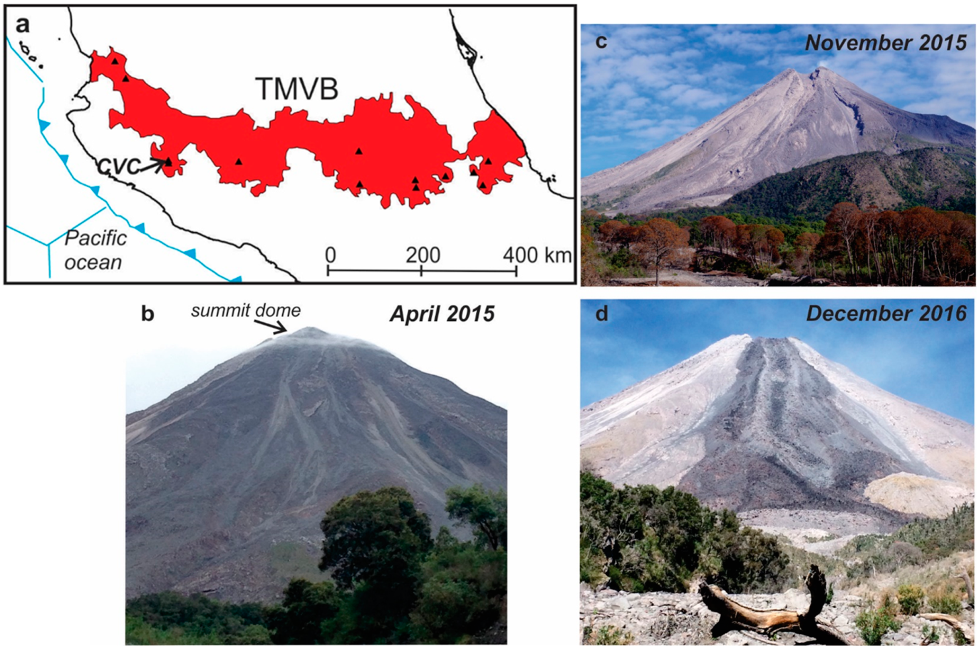
1. Introduction
2. Chronology of the Eruptive Phases Prior to, During and After the 10–11 July 2015 Climatic Event
3. Data
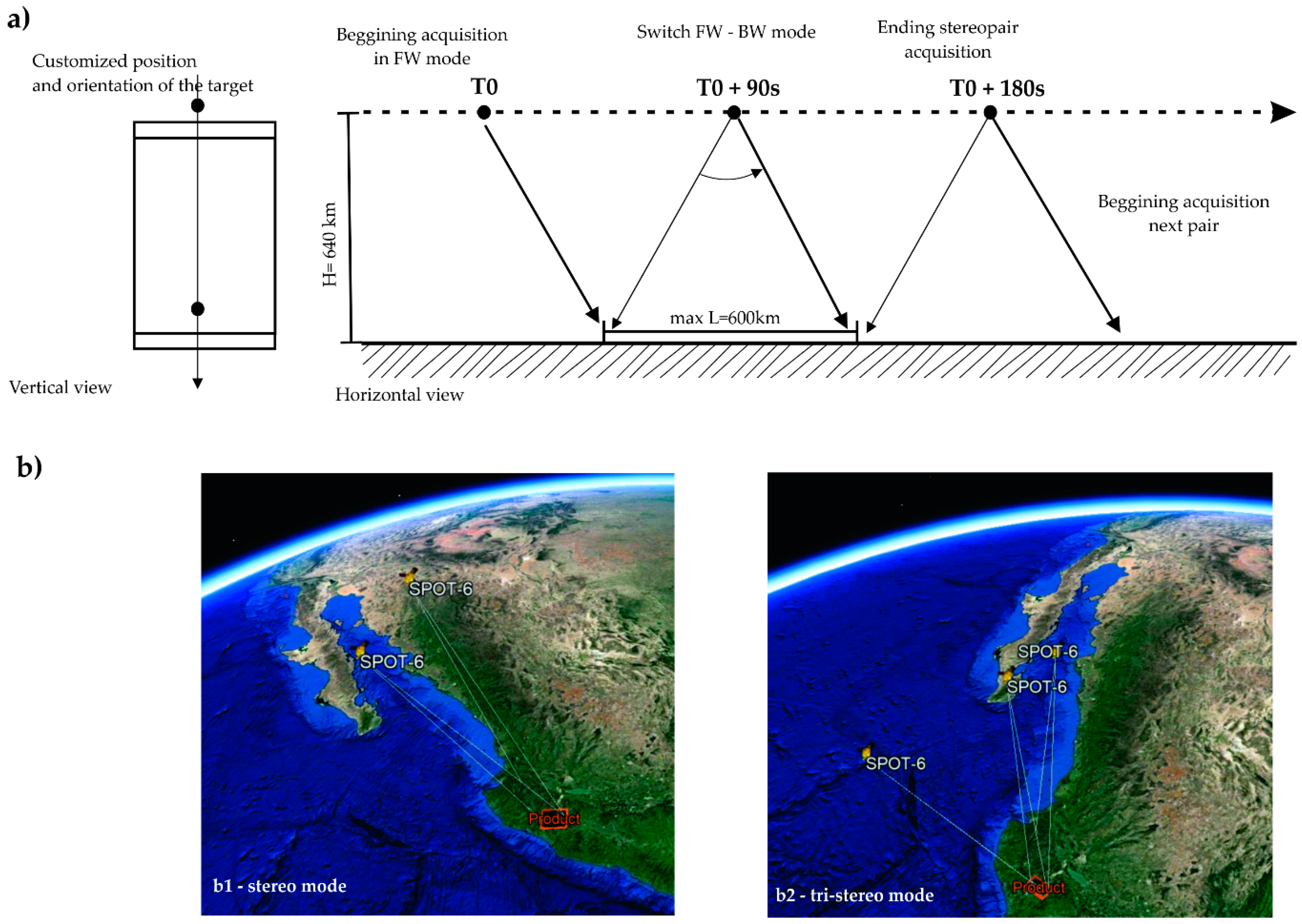
3.1. SPOT 6/7 Constellation
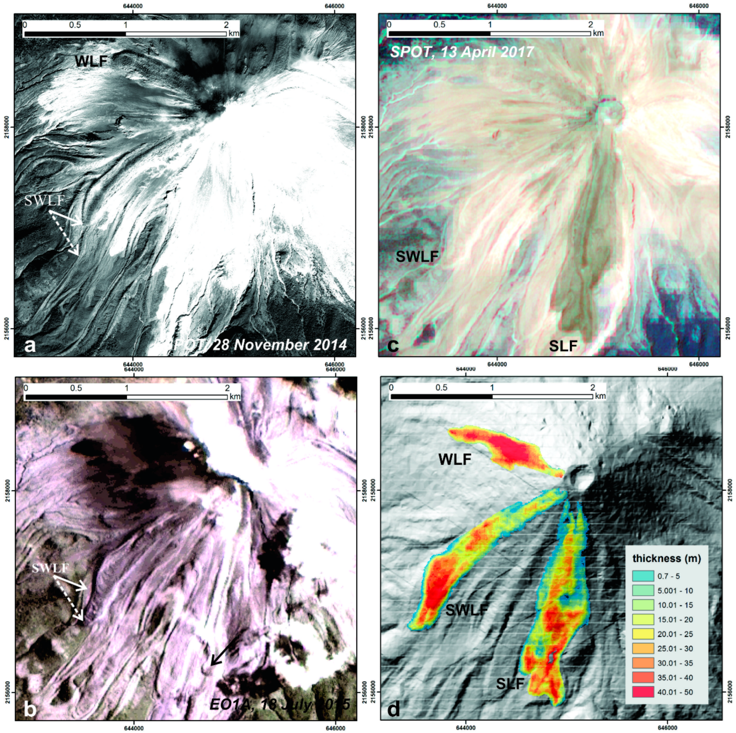
3.2. Remote Sensing Data (EO-1 (ALI) and SPOT 6/7) Used for the Interpretation of the Eruptive Temporal Sequence
4. Methods
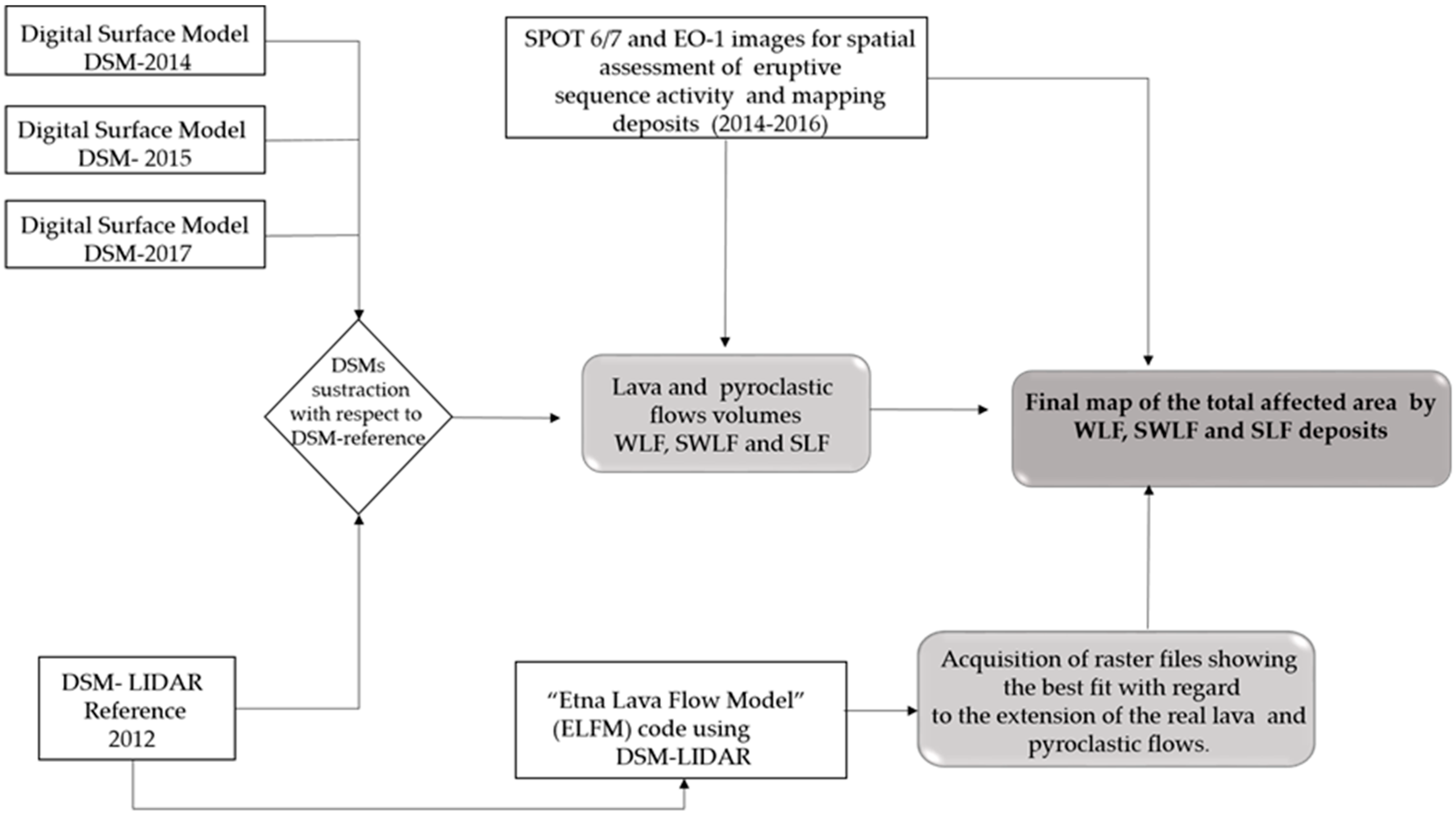
4.1. Digital Surface Models (DSM) Processing
4.2. Volume Estimation of the Associated Lava Flows and Pyroclastic Flows
4.3. Using the Etna Lava Flow Model Simulation Code
5. Results
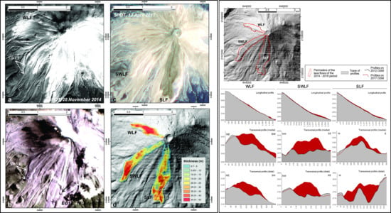
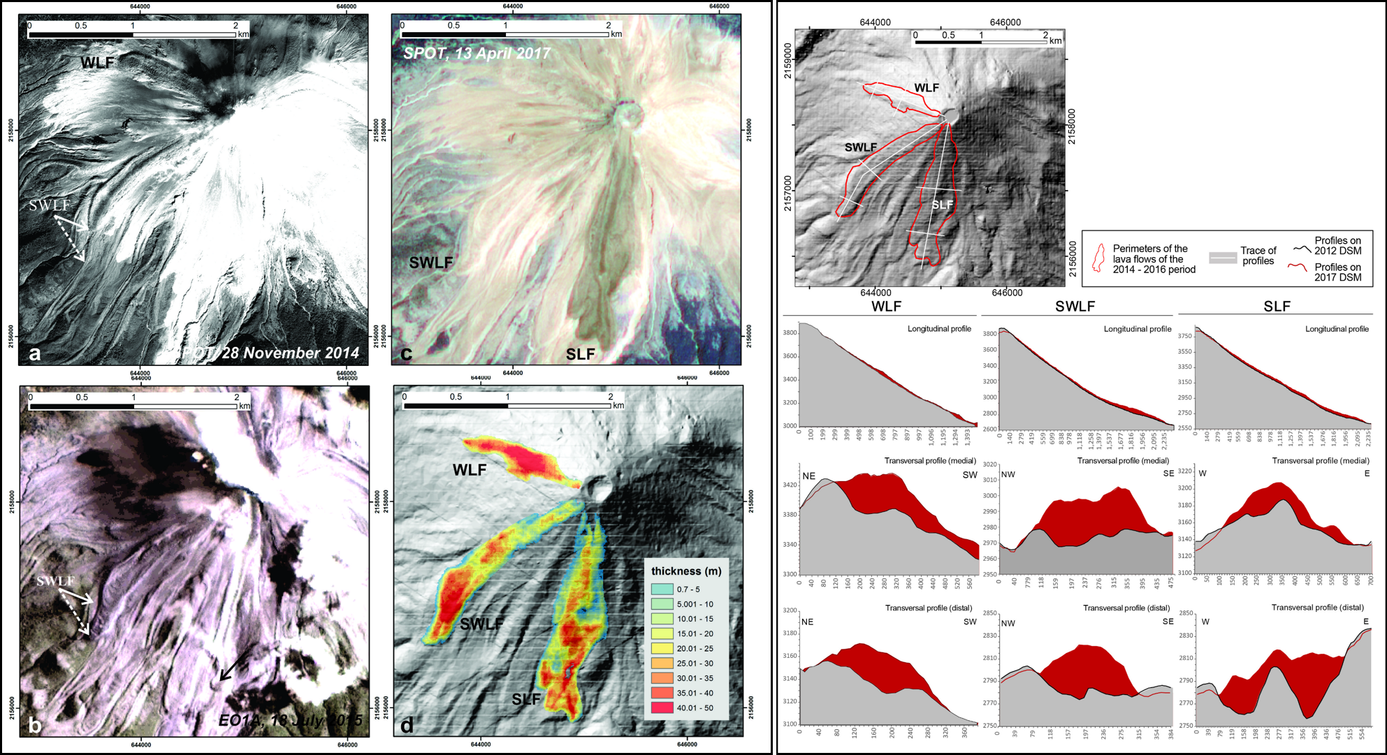
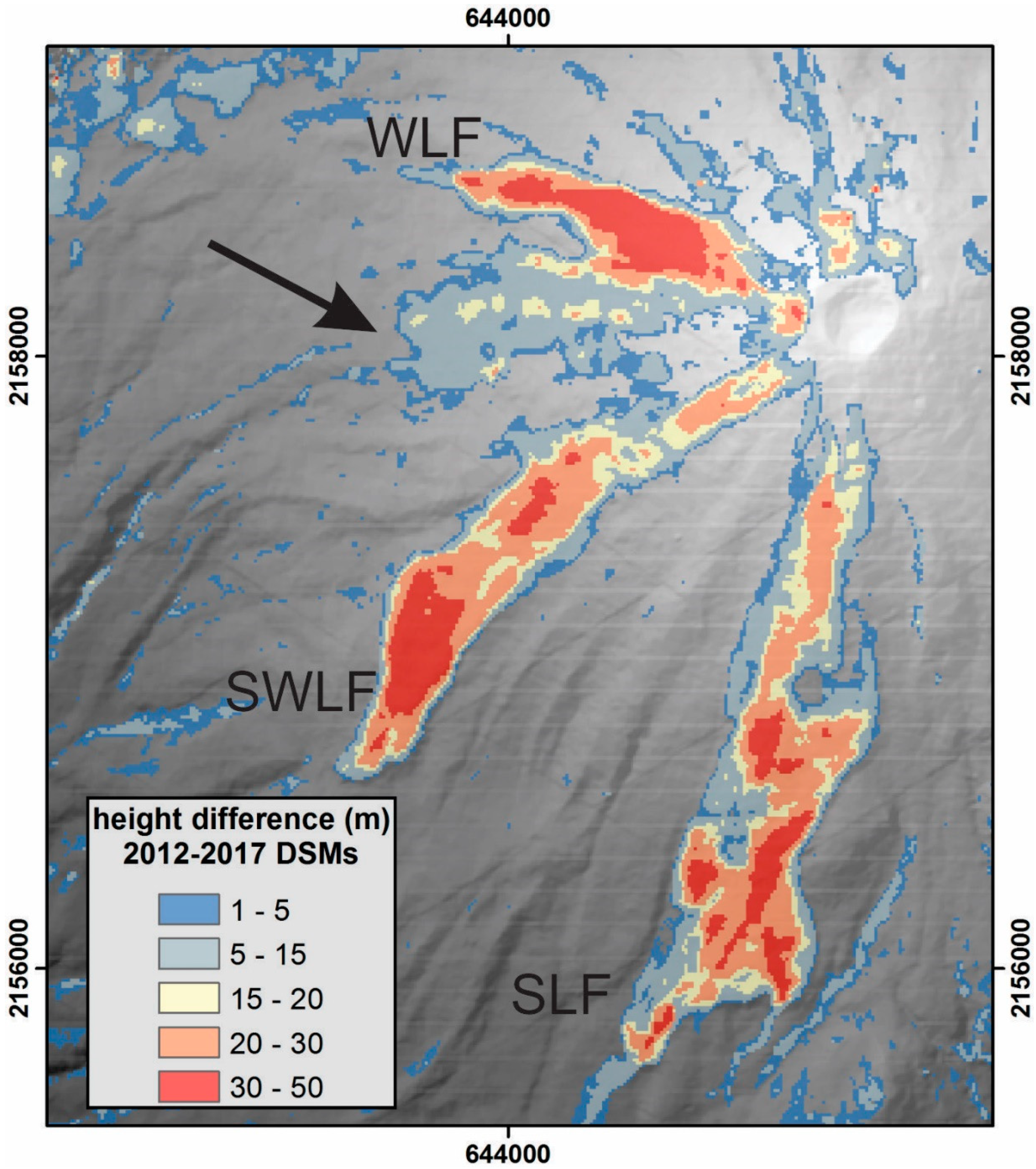
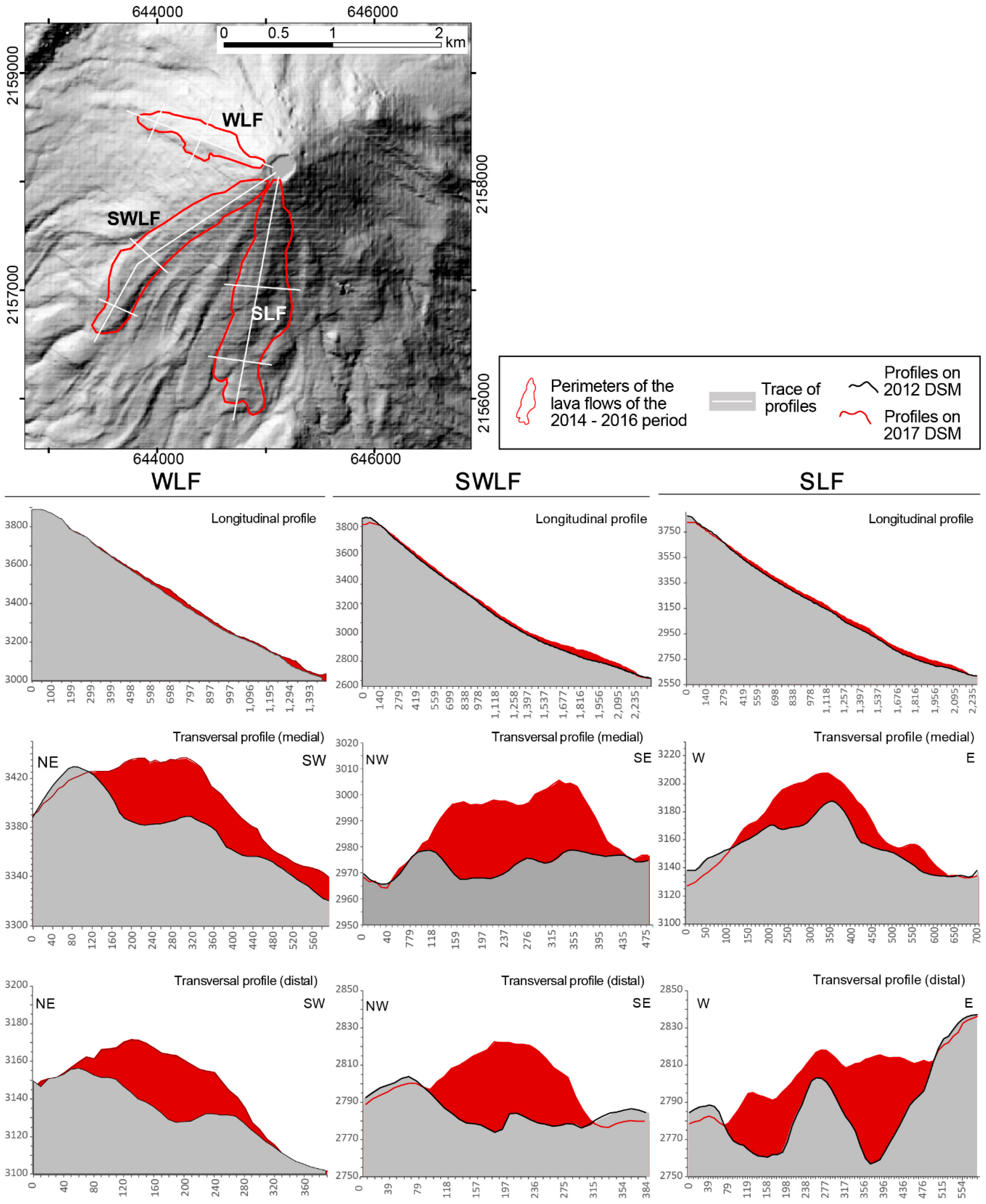
5.1. Lava Flow Inundation Area and Volume Estimation
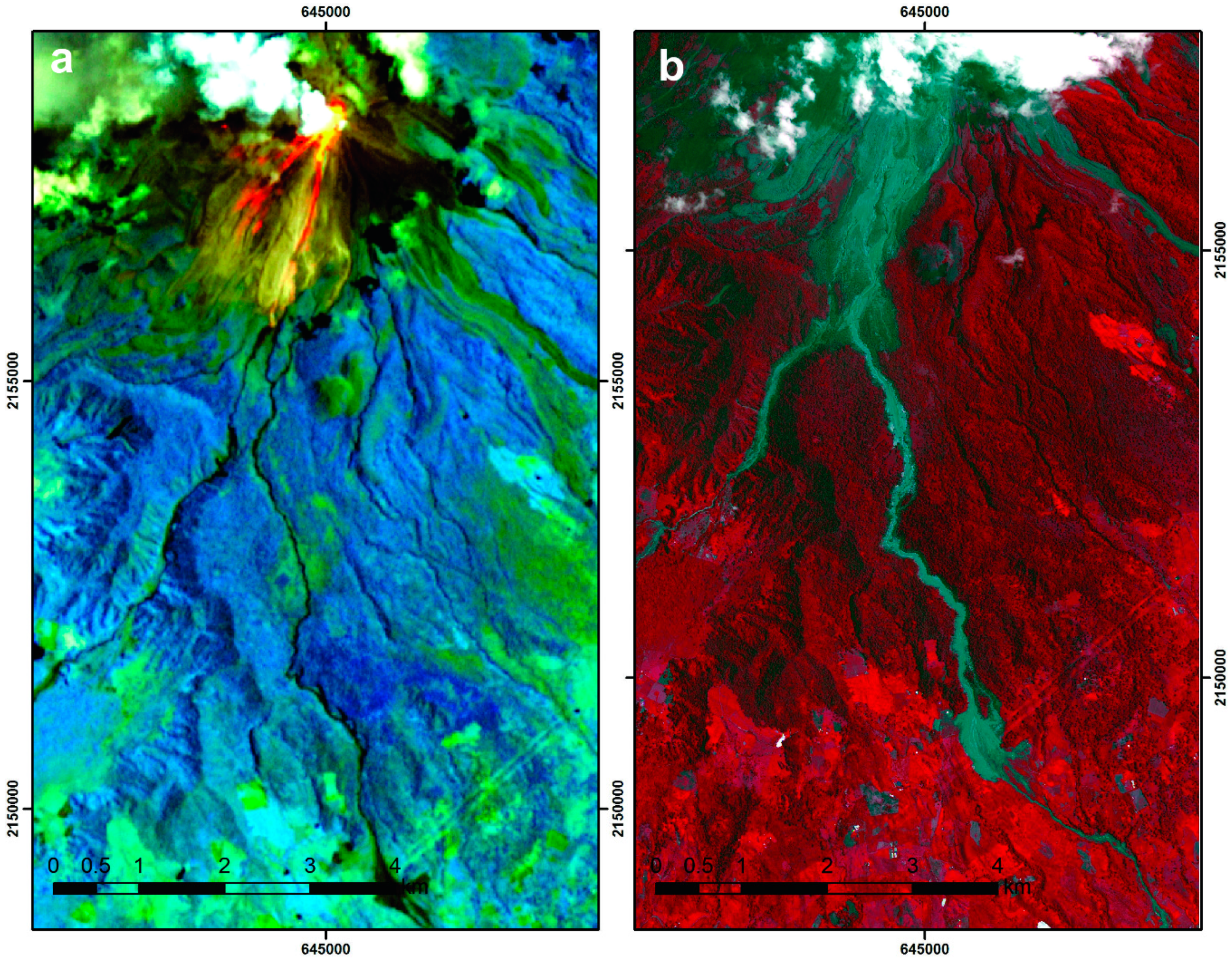
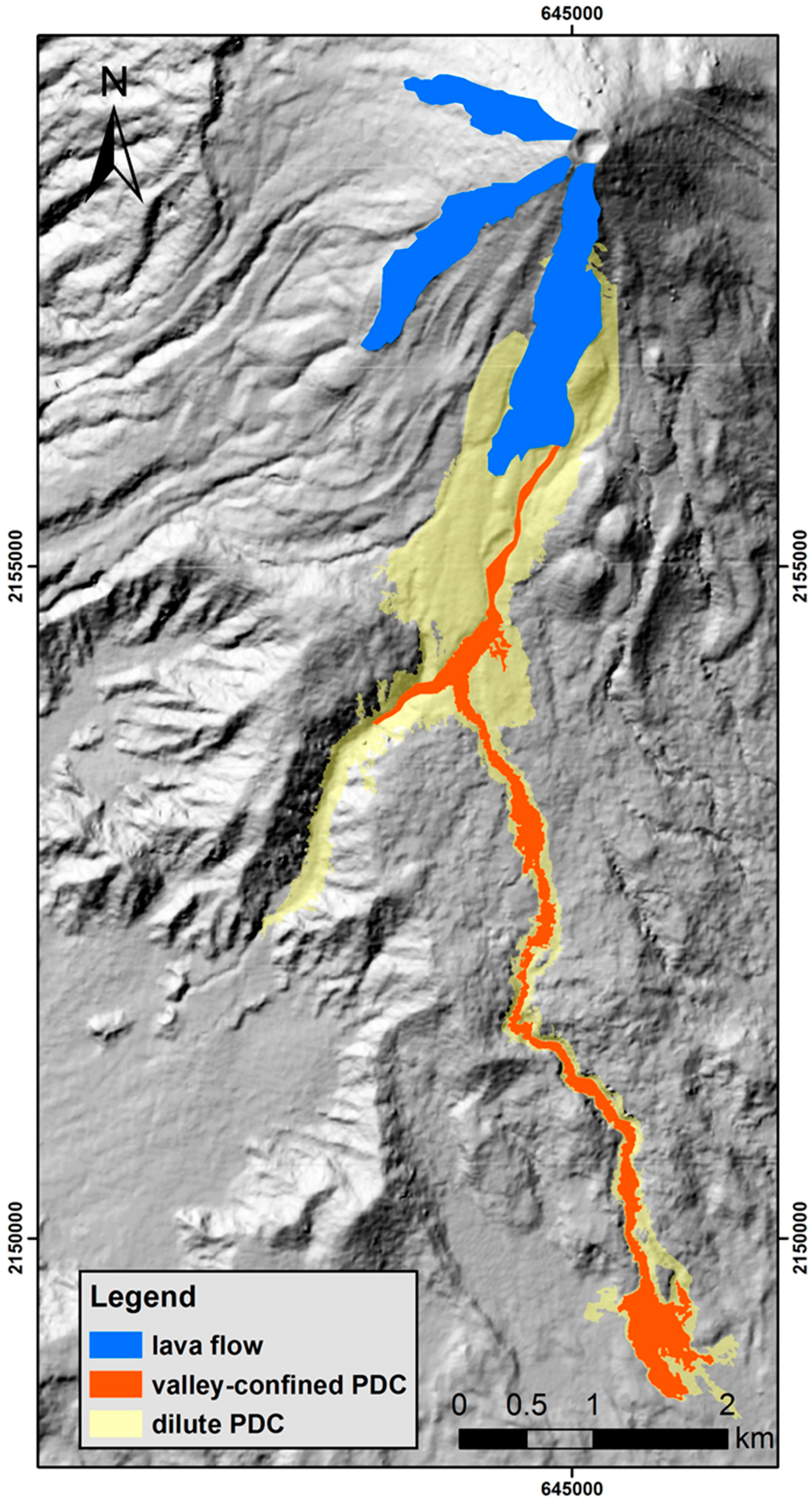
5.2. Block-and-Ash Flow Deposits: Inundation Limits, Volume and Thickness Variation
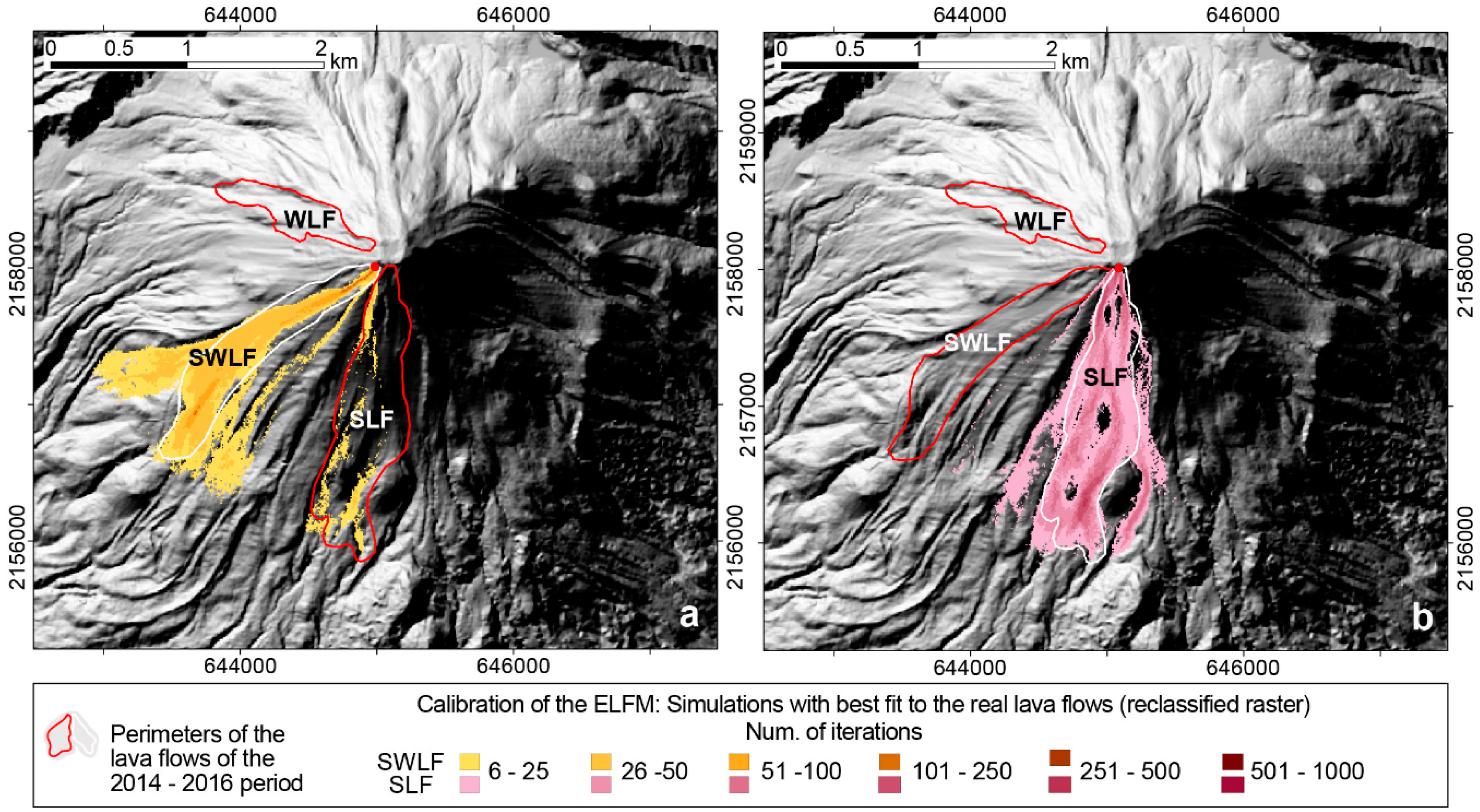
5.3. Calibration of the ELFM at the Colima Volcano
6. Discussion
7. Conclusions
Author Contributions
Funding
Acknowledgments
Conflicts of Interest
Glossary
| ASCII | American Standard Code for Information Interchange |
| ASTER | Advanced Spaceborne Thermal Emission and Reflection Radiometer |
| BAF | block-and-ash flow |
| BW | switches to backward acquisition |
| DEM | Digital Elevation Model |
| DRE | dense rock equivalent |
| DSM | Digital Surface Model |
| ELFM | Etna Lava Flow Model (code) |
| EO-1 (ALI) | Earth Observing-1 ALI (on) Advanced Land Imager |
| ERMEX | Estación de Recepción México |
| FW | forward acquisition |
| GCP | ground control points |
| INEGI | National Institute of Geography and Statistics |
| InSAR | Interferometry Synthetic Aperture Radar |
| ITHACA | Information Technology for Humanitarian Assistance, Cooperation and Action |
| LIDAR | Light Detection and Ranging Data |
| PDC | Pyroclastic Density Currents |
| RMSE | root mean squared error |
| RPC | rational polynomial coefficients |
| SLF | south lava flow |
| SPOT | Satellite Pour l’Observation de la Terre (SPOT/6) |
| SWLF | South-West Lava Flow |
| UNITAR | United Nations Institute for Training and Research |
| UNOSAT | UNITAR Operational Satellite Applications Programme |
| UTM | Universal Transversal of Mercator |
| WLF | West Lava Flow |
References
- Luhr, J.F.; Carmichael, I.S.E. The Colima Volcanic Complex, México. Contrib. Mineral. Petrol. 1981, 76, 127–147. [Google Scholar] [CrossRef]
- Medina, F. Analysis of the eruptive history of the Volcán Colima, México, 1560–1980. Geof. Int. 1983, 22, 157–178. [Google Scholar]
- De la Cruz-Reyna, S. Random patterns of occurrence of explosive eruptions at Colima volcano, México. J. Volcanol. Geotherm. Res. 1993, 55, 51–68. [Google Scholar] [CrossRef]
- Macias, J.L.; Saucedo, R.; Gavilanes-Ruiz, J.C.; Varley, N.; Velasco-Garcia, S.; Bursik, M.I.; Vargas-Gutierres, V.; Cortes, A. Flujos piroclásticos asociados a la actividad explosiva del volcán de Colima y perspectivas futuras. GEOS 2006, 25, 340–351. [Google Scholar]
- Sulpizio, R.; Capra, L.; Sarocchi, D.; Saucedo, R.; Gavilanes, J.C.; Varley, N.R. Predicting the block-and-ash flow inundation areas at Volcán de Colima (Colima, Mexico) based on the present day (February 2010) status. J. Volcanol. Geotherm. Res. 2010, 193, 49–66. [Google Scholar] [CrossRef]
- Capra, L.; Macías, J.L.; Cortés, A.; Dávila, N.; Saucedo, R.; Osorio-Ocampo, S.; Arce, J.L.; Gavilanes-Ruiz, J.C.; Corona-Chávez, P.; García-Sánchez, L.; et al. Preliminary report on the July 10–11, 2015 eruption at Volcán de Colima: Pyroclastic, density currents with exceptional runouts and volume. J. Volcanol. Geotherm. Res. 2016, 310, 39–49. [Google Scholar] [CrossRef]
- Reyes-Dávila, G.; Arámbula-Mendoza, R.; Espinasa-Pereña, R.; Pankhurst, M.J.; Navarro-Ochoa, C.; Savov, I.; Vargas-Bracamontes, D.M.; Cortés-Cortés, A.; Gutiérrez-Martínez, C.; Valdés-González, C.; et al. Volcán de Colima dome collapse of July, 2015 and associated pyroclastic density currents. J. Volcanol. Geotherm. Res. 2016, 320, 100–106. [Google Scholar] [CrossRef] [Green Version]
- Saucedo, R.; Macias, J.L.; Gavilanes, J.C.; Arce, J.L.; Komorowski, J.C.; Gardner, J.E.; Valdez, G. Corrigendum to Eyewitness, stratigraphy, chemistry, and eruptive dynamics of the 1913 Plinian eruption of Volcan de Colima, Mexico. J. Volcanol. Geotherm. Res. 2010, 191, 149–166. [Google Scholar] [CrossRef]
- Capra, L.; Gavilanes-Ruiz, J.C.; Bonasia, R.; Saucedo-Giron, R.; Sulpizio, R. Re-assessing volcanic hazard zonation of Volcán de Colima, México. Nat. Hazards 2014, 76, 41–51. [Google Scholar] [CrossRef]
- Harris, A.J.L.; Butterworth, A.L.; Carlton, R.W.; Downey, I.; Miller, P.; Navarro, P.; Rothery, D.A. Low-cost volcano surveillance from space: Case studies from Etna, Krafla, Cerro Negro, Fogo, Lascar and Erebus. Bull. Volcanol. 1997b, 59, 49–64. [Google Scholar] [CrossRef]
- Harris, A.J.L. Thermal Remote Sensing of Active Volcanoes, a User’s Manual; Cambridge University Press: Cambridge, UK, 2013; p. 736. [Google Scholar]
- Ramsey, M.S.; Harris, A.J.L. Volcanology 2020: How will thermal remote sensing of volcanic surface activity evolve over the next decade? J. Volcanol. Geotherm. Res. 2013, 249, 217–233. [Google Scholar] [CrossRef]
- Harris, A.J.L.; Rowland, S.K. FLOWGO: A kinematic thermo-rheological model for lava flowing in a channel. Bull. Volcanol. 2001, 63, 20–44. [Google Scholar] [CrossRef]
- Wright, R.; Garbeil, H.; Harris, A.J.L. Using infrared satellite data to drive a thermo-rheological/stochastic lava flow emplacement model: A method for near-real-time volcanic hazard assessment. Geophys. Res. Lett. 2008, 35, L19307. [Google Scholar] [CrossRef]
- Oppenheimer, C. Lava Flow Cooling Estimated from Landsat Thematic Mapper Infrared Data: The Lonquimay Eruption (Chile, 1989). J. Geophys. Res. 1991, 96, B13. [Google Scholar] [CrossRef]
- Aufaristama, M.; Hoskuldsson, A.; Orn Ulfarsson, M.; Jonsdottir, I.; Thordarson, T. The 2014–2015 Lava Flow Field at Holuhraun, Iceland: Using Airborne Hyperspectral Remote Sensing for Discriminating the Lava Surface. Remote Sens. 2019, 11, 476. [Google Scholar] [CrossRef]
- Pallister, J.; Wessels, R.; Griswold, J.; McCausland, W.; Kartadinata, N.; Gunawan, H.; Budianto, A.; Primulyana, S. Monitoring, forecasting collapse events, and mapping pyroclastic deposits at Sinabung volcano with satellite imagery. J. Volcanol. Geotherm. Res. 2018. [Google Scholar] [CrossRef]
- Bonny, E.; Thordarson, T.; Wright, R.; Höskuldsson, A.; Jónsdóttir, I. The Volume of Lava Erupted During the 2014 to 2015 Eruption at Holuhraun, Iceland: A Comparison Between Satellite- and Ground-Based Measurements. J. Geophys. Res. Solid Earth 2018, 123, 5412–5426. [Google Scholar] [CrossRef]
- Dietterich, H.R.; Poland, M.P.; Schmidt, D.A.; Cashman, K.V.; Sherrod, D.R.; Espinosa, A.T. Tracking lava flow emplacement on the east rift zone of Kīlauea, Hawai‘i, with synthetic aperture radar coherence. Geochem. Geophys. Geosyst. 2012, 13, 5. [Google Scholar] [CrossRef]
- Schaefer, L.; Lu, Z.; Oommen, T. Post-Eruption Deformation Processes Measured Using ALOS-1 and UAVSAR InSAR at Pacaya Volcano, Guatemala. Remote Sens. 2016, 8, 73. [Google Scholar] [CrossRef]
- McAlpin, D.B.; Meyer, F.J.; Gong, W.; Beget, J.E.; Webley, P.W. Pyroclastic Flow Deposits and InSAR: Analysis of Long-Term Subsidence at Augustine Volcano, Alaska. Remote Sens. 2016, 9, 4. [Google Scholar] [CrossRef]
- Cando, M.; Martínez, A. Determination of Primary and Secondary Lahar Flow Paths of the Fuego Volcano (Guatemala) Using Morphometric Parameters. Remote Sens. 2019, 11, 727. [Google Scholar] [CrossRef]
- GVP. Report on Colima (Mexico). In Weekly Volcanic Activity Report, 19 November–25 November 2014; Smithsonian Institution: Washington, DC, USA; US Geological Survey: Reston, VA, USA, 2014. [Google Scholar]
- GVP. Report on Colima (Mexico). In Weekly Volcanic Activity Report, 7 January–13 January 2015; Smithsonian Institution: Washington, DC, USA; US Geological Survey: Reston, VA, USA, 2015. [Google Scholar]
- GVP. Report on Colima (Mexico). In Weekly Volcanic Activity Report, 18 February–24 February 2015; Smithsonian Institution: Washington, DC, USA; US Geological Survey: Reston, VA, USA, 2015. [Google Scholar]
- GVP. Report on Colima (Mexico). In Weekly Volcanic Activity Report, 13 May–19 May 2015; Smithsonian Institution: Washington, DC, USA; US Geological Survey: Reston, VA, USA, 2015. [Google Scholar]
- GVP. Report on Colima (Mexico). In Weekly Volcanic Activity Report, 8 July–14 July 2015; Smithsonian Institution: Washington, DC, USA; US Geological Survey: Reston, VA, USA, 2015. [Google Scholar]
- Macorps, E.; Charbonnier, S.J.; Varley, N.R.; Capra, L.; Atlas, Z.; Cabré, J. Stratigraphy, sedimentology and inferred flow dynamics from the July 2015 block-and-ash flow deposits at Volcán de Colima, Mexico. J. Volcanol. Geotherm. Res 2018, 349, 99–116. [Google Scholar] [CrossRef]
- Pensa, A.; Capra, L.; Giordano, G.; Corrado, S. Emplacement temperature estimation of the 2015 dome collapse of Volcán de Colima as key proxy for flow dynamics of confined and unconfined pyroclastic density currents. J. Volcanol. Geotherm. Res. 2018, 357, 321–338. [Google Scholar] [CrossRef]
- GVO. Global Volcanism Program, 2016. Report on Colima (Mexico). In Weekly Volcanic Activity Report, 28 September–4 October 2016; Smithsonian Institution: Washington, DC, USA; US Geological Survey: Reston, VA, USA, 2016. [Google Scholar]
- GVO. Global Volcanism Program, 2016. Report on Colima (Mexico). In Weekly Volcanic Activity Report, 19 October–25 October 2016; Smithsonian Institution: Washington, DC, USA; US Geological Survey: Reston, VA, USA, 2016. [Google Scholar]
- Astrium and Eads company: The SPOT 6 & SPOT 7 Imagery User Guide. Available online: http://www.intelligence-airbusds.com/en/5280-spot-6-technical-documents (accessed on 30 October 2018).
- Davies, A.G.; Chien, S.; Baker, V. Monitoring active volcanism with the Autonomous Sciencecraft experiment on EO-1. Remote Sens. Environ. 2006, 101, 427–446. [Google Scholar] [CrossRef]
- NASA Earth Observatory. Available online: https://earthobservatory.nasa.gov/images/51583/volcanic-acitivity-at-krakatau (accessed on 14 April 2019).
- Davies, A.G.; Chien, S.; Doubleday, J.; Tran, D.; Thordarson, T.; Gudmundsson, M.T.; Höskuldsson, A.; Jakobsdóttir, S.S.; Wright, R.; Mandl, D. Observing Iceland’s Eyjafjallajo¨kull 2010 eruptions with the autonomous NASA Volcano Sensor Web. J. Geophys. Res. 2013, 118, 1–21. [Google Scholar] [CrossRef]
- Patrick, M.R.; Kauahikaua, T.; Orr, A. Operational thermal remote sensing and lava flow monitoring at the Hawaiian Volcano Observatory. In Detecting, Modelling and Responding to Effusive Eruptions; Geological Society: London, UK, 2016; Volume 426, p. 489. [Google Scholar]
- Mexican National Institute of Statistics and Geography-INEGI: Digital Elevation Model. Available online: http://www.beta.inegi.org.mx/app/geo2/elevacionesmex (accessed on September 2018).
- Lira, J. Tratamiento Digital de Imágenes, 3rd ed.; Ciudad de México: Mexico City, Mexico, 2018; pp. 235–318. [Google Scholar]
- Damiani, M.L.; Groppelli, G.; Norini, G.; Bertino, E.; Gigliuto, A.; Nucita, A. A lava flow simulation model for the development of volcanic hazard maps for Mount Etna (Italy). Comput. Geosci. 2006, 32, 512–526. [Google Scholar] [CrossRef]
- Martin Del Pozzo, A.L.; Alatorre, M.; Arana, L.; Bonasia, R.; Capra, L.; Cassata, W.; Córdoba, G.; Cortés, J.; Delgado, H.; Ferrés, M.D.; et al. Memoria Técnica del Mapa de Peligros del Volcán Popocatépetl, 1st ed.; Monografías del Instituto de Geofísica, Universidad Nacional Autónoma de México: Mexico City, Mexico, 2008; p. 166. [Google Scholar]
- Sieron, K.; Ferrés, D.; Siebe, C.; Constantinescu, R.; Capra, L.; Connor, C.; Connor, L.; Gropelli, G.; González-Zuccolotto, K. Ceboruco hazard map: Part II—modeling volcanic phenomena and construction of the general hazard map. Nat. Hazards 2019. [Google Scholar] [CrossRef]
- Costa, A.; Macedonio, G. Computational modeling of lava flows: A review. In Kinematics and Dynamics of Lava Flows, 1st ed.; Geological Society of America: Boulder, CO, USA, 2005; pp. 209–218. [Google Scholar]
- Favalli, M.; Tarquini, S.; Fornaciai, A. DOWNFLOW code and LIDAR technology for lava flow analysis and hazard assessment at Mount Etna. Ann. Geophys. 2011, 54, 552–566. [Google Scholar] [CrossRef]
- Bertino, E.; Damiani, M.L.; Groppelli, G.; Norini, G.; Aldighieri, B.; Borgonovo, S.; Comoglio, F.; Pasquaré, G. Modelling lava flow to assess hazard on Mount Etna (Italy). From geological data to a preliminary hazard map. In Proceedings of the iEMSs; International Environmental Modelling and Software Society: Burlington, NJ, USA, 2006; pp. 1–8. [Google Scholar]
- Felpeto, A.; Araña, V.; Ortiz, R.; Astiz, M.; García, A. Assessment and modelling of lava flow hazard on Lanzarote (Canary Islands). Nat. Hazards 2001, 23, 247–257. [Google Scholar] [CrossRef]
- Connor, L.; Connor, C.B.; Meliksetian, K.; Savov, I. Probabilistic approach to modeling lava flow inundation: A lava flow hazard assessment for a nuclear facility in Armenia. J. Appl. Volcanol. 2012, 1, 1–19. [Google Scholar] [CrossRef]
- Aldighieri, B.; Groppelli, G.; Norini, G.; Bertino, E.; Borgonovo, S.; Comoglio, F.; Pasquaré, G. Proposta di una metodología per la valutazione della pericolositá vulcanica del Monte Etna. Rend. Soc. Geol. It. 2007, 4, 23–25. [Google Scholar]
- Stevens, N.F.; Manville, V.; Heron, D.W. The sensitivity of a volcanic flow model to digital elevation model accuracy: Experiments with.zed map contours and interferometric SAR at Ruapehu and Taranaki volcanoes, New Zealand. J. Volcanol. Geotherm. Res. 2002, 119, 89–105. [Google Scholar] [CrossRef]
- Claessens, L.; Heuvelink, G.B.M.; Schoorl, J.M.; Veldkamp, A. DEM resolution effects on shallow landslide hazard and soil redistribution modeling. Earth Surf. Process. Landf. 2005, 30, 461–477. [Google Scholar] [CrossRef]
- Capra, L.; Manea, V.C.; Manea, M.; Norini, G. The importance of digital elevation model resolution on granular flow simulations: A test case for Colima volcano using TITAN2D computational routine. Nat. Hazards 2011, 59, 665–680. [Google Scholar] [CrossRef]
- Caballero, L.; Capra, L.; Vázquez, R. Evaluating the performance of FLO2D for simulating past lahar events at the most active Mexican volcanoes: Popocatépetl and Volcán de Colima. In Natural Hazard Uncertainty Assessment: Modeling and Decision Support; Geophys Monograph: Washington, DC, USA, 2017; Volume 223, pp. 179–189. [Google Scholar]
- Arámbula-Mendoza, R.; Reyes-Dávila, G.; Dulce, M.V.B.; González-Amezcua, M.; Navarro-Ochoa, C.; Martínez-Fierros, A.; Ramírez-Vázquez, A. Seismic monitoring of effusive-explosive activity and large lava dome collapses during 2013–2015 at Volcán de Colima, Mexico. J. Volcanol. Geotherm. Res 2018, 351, 75–88. [Google Scholar] [CrossRef]
- Zobin, V.; Varley, N.; Gonzalez, M.; Orozco, J. Monitoring the 2004 andesitic block-lava extrusion at Volcán de Colima, México from seismic activity and SO2 emission. J. Volcanol. Geotherm. Res 2008, 177, 367–377. [Google Scholar] [CrossRef]
- Pyle, D.M. Chapter 13—Sizes of Volcanic Eruptions. In The Encyclopedia of Volcanoes, 2nd ed.; Academic Press: San Francisco, CA, USA, 2015; Volume 1, pp. 257–263. [Google Scholar]
- Harris, J.L.; Rowland, S.K. Chapter 17—Lava Flows and Rheology. In The Encyclopedia of Volcanoes, 2nd ed.; Academic Press: San Francisco, CA, USA, 2015; Volume 1, pp. 321–342. [Google Scholar]
- Massaro, M.; Sulpizio, R.; Costa, A.; Capra, L.; Lucci, F. Understanding eruptive style variations at calc-alkaline volcanoes: The 1913 eruption of Fuego de Colima volcano (Mexico). Bull. Volcanol. 2018, 80, 62. [Google Scholar] [CrossRef]
- United Nations Institute for Training and Research (UNITAR-UNOSAT). Guatemala, Volcán de Fuego. Flujo piroclástico, 4 de Junio de 2018. Available online: https://unitar.org/unosat/node/44/2815?utm_source=unosat-unitar&utm_medium=rss&utm_campaign=maps (accessed on 15 October 2018).


| Satellite | Date | Mode | Orientation Angle | Incidence Angle | Image Resolution | DSM Resolution |
|---|---|---|---|---|---|---|
| SPOT6 | 28/11/2014 | Panchromatic with tri-stereo capacity * | +169.66° | +19.08° | 1.5 m | 10 m |
| SPOT6 | 28/11/2014 | Panchromatic with tri-stereo capacity | +74.31° | +8.22° | 1.5 m | |
| SPOT6 | 28/11/2014 | Panchromatic with tri-stereo capacity | +42.95° | +14.05° | 1.5 m | |
| SPOT6 | 27/07/2015 | Panchromatic with stereo capacity-duo stereo | +16.4° | 1.5 m | 21 m | |
| SPOT6 | 27/07/2015 | Panchromatic with stereo capacity-duo stereo | +16.8° | 1.5 m | ||
| SPOT6 | 11/04/2017 | Panchromatic with stereo capacity-duo stereo | +306.71° | +19.22° | 1.5 m | 7.5 m |
| SPOT6 | 29/04/2017 | Panchromatic with stereo capacity-duo stereo | +250.10° | +20.92° | 1.5 m |
| Sensor | Date | Spectral Mode | Pixel Resolution (m) | Level Acquisition |
|---|---|---|---|---|
| EO-1 (ALI) | 15/07/2015 | Multispectral | 10 | 1B |
| SPOT/6 | 25/07/2015 | Panchromatic/Multispectral | 1.5 10 | 1A |
| SPOT/7 | 13/04/2017 | Multispectral | 6 | 1A |
| DSM | RMS (m) | S2 | S | Number of Geodesic Stations (NGRS) Considered |
|---|---|---|---|---|
| Stereo-pair, 2017 | 0.281 | 0.07370655 | 0.27148951 | 63 |
| Stereo-pair, 2015 | 0.803 | 0.2833703 | 0.532325379 | 42 |
| Tri-stereo, 2014 | 1.2991 | 0.44845054 | 0.669664499 | 53 |
| Lava Flow | Date | Travel Distance (km) | Volume (m3) | Area (m2) | Error in Volume (m3) | Slope |
|---|---|---|---|---|---|---|
| LAVA W | May 2014 | 1.2 | 7.5 × 10⁶ | 2.3 × 10⁵ | ±3.45 × 10⁵ | 31° |
| LAVA SW | September 2014 | 2.2 | 4.7 × 10⁶ (by Nov. 2014) 12.2 × 10⁶ final | 5.6 × 10⁵ | ±7.8 × 10⁵ | 27.8° |
| LAVA S | September 2016 | 2.2 | 16 × 106 | 8.1 × 10⁵ | ±1.1 × 10⁶ | 29.5° |
© 2019 by the authors. Licensee MDPI, Basel, Switzerland. This article is an open access article distributed under the terms and conditions of the Creative Commons Attribution (CC BY) license (http://creativecommons.org/licenses/by/4.0/).
Share and Cite
Dávila, N.; Capra, L.; Ferrés, D.; Gavilanes-Ruiz, J.C.; Flores, P. Chronology of the 2014–2016 Eruptive Phase of Volcán de Colima and Volume Estimation of Associated Lava Flows and Pyroclastic Flows Based on Optical Multi-Sensors. Remote Sens. 2019, 11, 1167. https://doi.org/10.3390/rs11101167
Dávila N, Capra L, Ferrés D, Gavilanes-Ruiz JC, Flores P. Chronology of the 2014–2016 Eruptive Phase of Volcán de Colima and Volume Estimation of Associated Lava Flows and Pyroclastic Flows Based on Optical Multi-Sensors. Remote Sensing. 2019; 11(10):1167. https://doi.org/10.3390/rs11101167
Chicago/Turabian StyleDávila, Norma, Lucia Capra, Dolors Ferrés, Juan Carlos Gavilanes-Ruiz, and Pablo Flores. 2019. "Chronology of the 2014–2016 Eruptive Phase of Volcán de Colima and Volume Estimation of Associated Lava Flows and Pyroclastic Flows Based on Optical Multi-Sensors" Remote Sensing 11, no. 10: 1167. https://doi.org/10.3390/rs11101167