Framework for Mapping Integrated Crop-Livestock Systems in Mato Grosso, Brazil

Abstract

Integrated crop-livestock (ICL) systems combine livestock and crop production in the same area, increasing the efficiency of land use and machinery, while mitigating greenhouse gas emissions, and reducing production risks, plant diseases and pests. ICL systems are primarily divided into annual (ICLa) and multi-annual (ICLm) systems. Projects such as the “Integrated crop-livestock-forest Network” and the “Livestock Rally” have estimated the ICL areas for Brazil on a state or regional basis. However, it remains necessary to create methods for spatial identification of ICL areas. Thus, we developed a framework for mapping ICL areas in Mato Grosso, Brazil using the Enhanced Vegetation Index time-series of Moderate Resolution Imaging Spectroradiometer and a Time-Weighted Dynamic Time Warping (TWDTW) classification method. The classification of ICL areas occurred in three phases. Phase 1 corresponded to the classification of land use from 2008 to 2016. In Phase 2, the ICLa areas were identified. Finally, Phase 3 corresponded to the ICLm identification. The framework showed overall accuracies of 86% and 92% for ICL areas. ICLm accounted for 87% of the ICL areas. Considering only agricultural areas or only pasture areas, ICL systems represented 5% and 15%, respectively.

1. Introduction

The need to increase food production and the restriction of agricultural expansion by environmental policies led to the adoption of production systems with higher productivity and lower environmental impacts, such as integrated crop-livestock (ICL) systems [1,2,3,4,5]. These systems employ strategies that aim to increase the land production such as, the integrated use of land as pastures for livestock and crop activities in succession, rotation, or intercropping [6,7,8]. In Brazil, ICL systems are associated with an improvement in pasture conditions and an intensification in land use [3,9,10]. The Brazilian Agriculture Ministry is aiming for four million new ICL areas by 2020 as part of the Brazilian Low Carbon Agriculture Plan—ABC Plan [11].

The interaction between crop and livestock makes the nutrient cycle more efficient, improves soil quality, and increases overall productivity [12,13,14]. Thus, integrated systems increase land and machinery efficiency, mitigate greenhouse gas emissions, and reduce production risks, plant diseases, and pests [15,16]. The ICL systems can be divided into two groups, annual and multi-annual [6]. In the annual group, land is used for grain cultivation in summer and pasture cultivation for livestock in winter. In the multi-annual ICL systems, usually for pasture reform, crop and pasture are cultivated in different years in rotation or succession.

The “Integrated crop-livestock-forest network” project (“Rede Integração-Lavoura-Pecuária”) conducted interviews to estimate the extent of the ICL system areas in Brazil on a state scale [17]. With the support of the “ABC Plan”, the “Livestock Rally” project performs fieldwork campaigns to understand and quantify livestock production and ICL systems in select regions in Brazil. Gil et al. [10] quantified farms with different ICL system combinations on a municipal scale in the Brazilian state of Mato Grosso. Despite these efforts to quantify ICL areas throughout Brazil, it is necessary to develop a framework to identify the spatial distribution of ICL areas within the municipalities. Remote sensing is an alternative approach for the systematic identification of ICL areas.

Remote sensing time-series are widely used to map agricultural land use and dynamics [18,19,20,21]. Vegetation index time-series show consistent results in the classification of pasture and crop areas [22,23,24,25,26,27]. It is also used to study land-use changes, detecting different land-use patterns in the same year (e.g., summer-crop and winter-crop) and over several years [28,29,30,31,32,33].

Many time-series classification methods have been developed to identify land use through remote sensing time-series [20,34,35,36]. Among these methods, Maus et al. [29] developed a Time-Weighted Dynamic Time Warping (TWDTW) method that improves the land-use classification in different years. To improve the land-use classification within the same year, they used a Moderate Resolution Imaging Spectroradiometer (MODIS) vegetation index time-series. The TWDTW method involves comparing two time-series, finding the optimal time-alignment, and then generating a measure of the dissimilarity (TWDTW distance), in which lower values indicate a greater similarity in the time-series temporal behavior. The use of a vegetation index times-series and a TWDTW classification method showed effectiveness compared with other classification methods, such as random forests [37].

Therefore, this study aims to develop a framework for mapping ICL system areas in a region of Brazil using vegetation index time-series from MODIS and a TWDTW classification method.

2. Materials and Methods

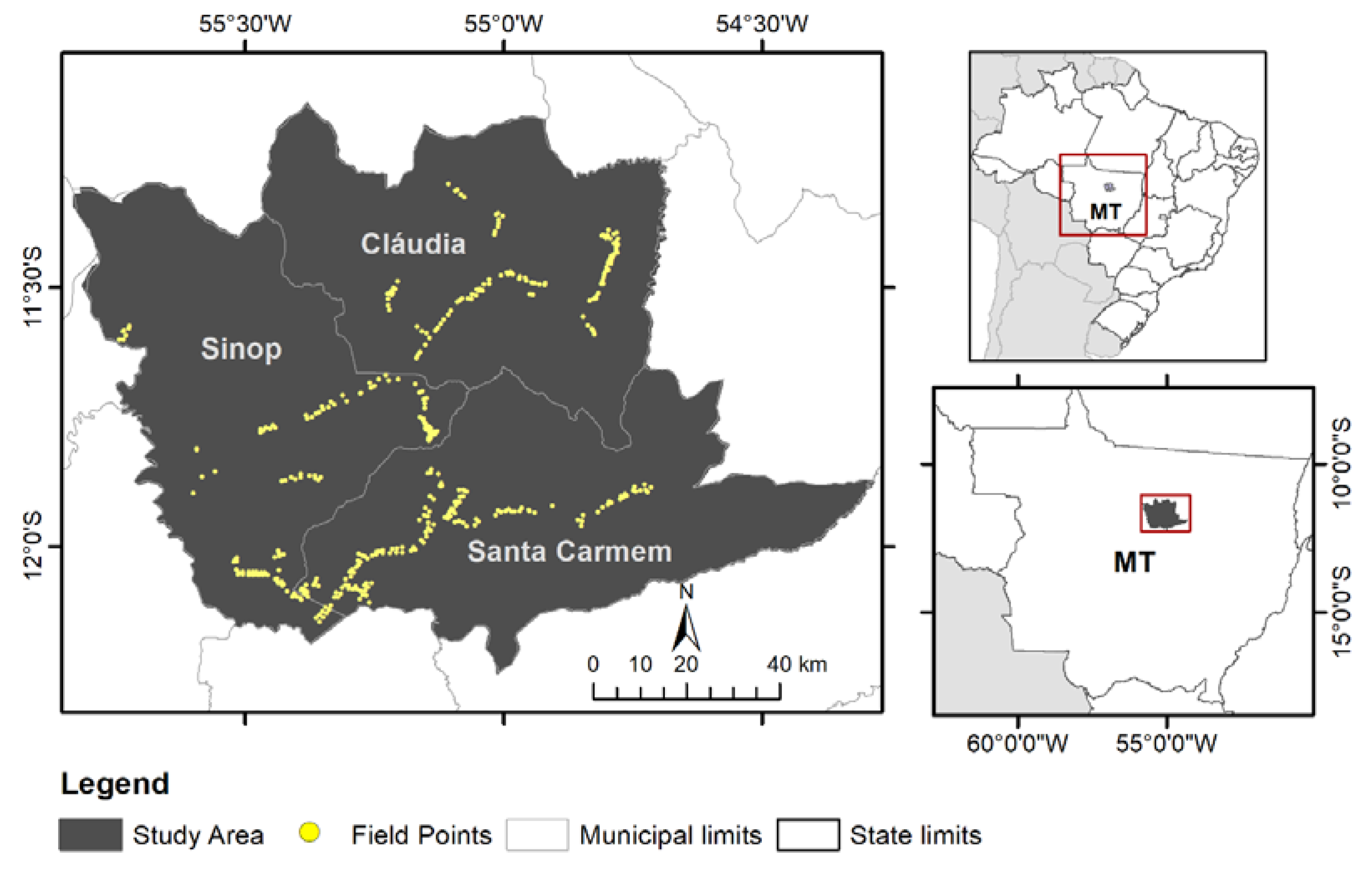
2.1. Study Area

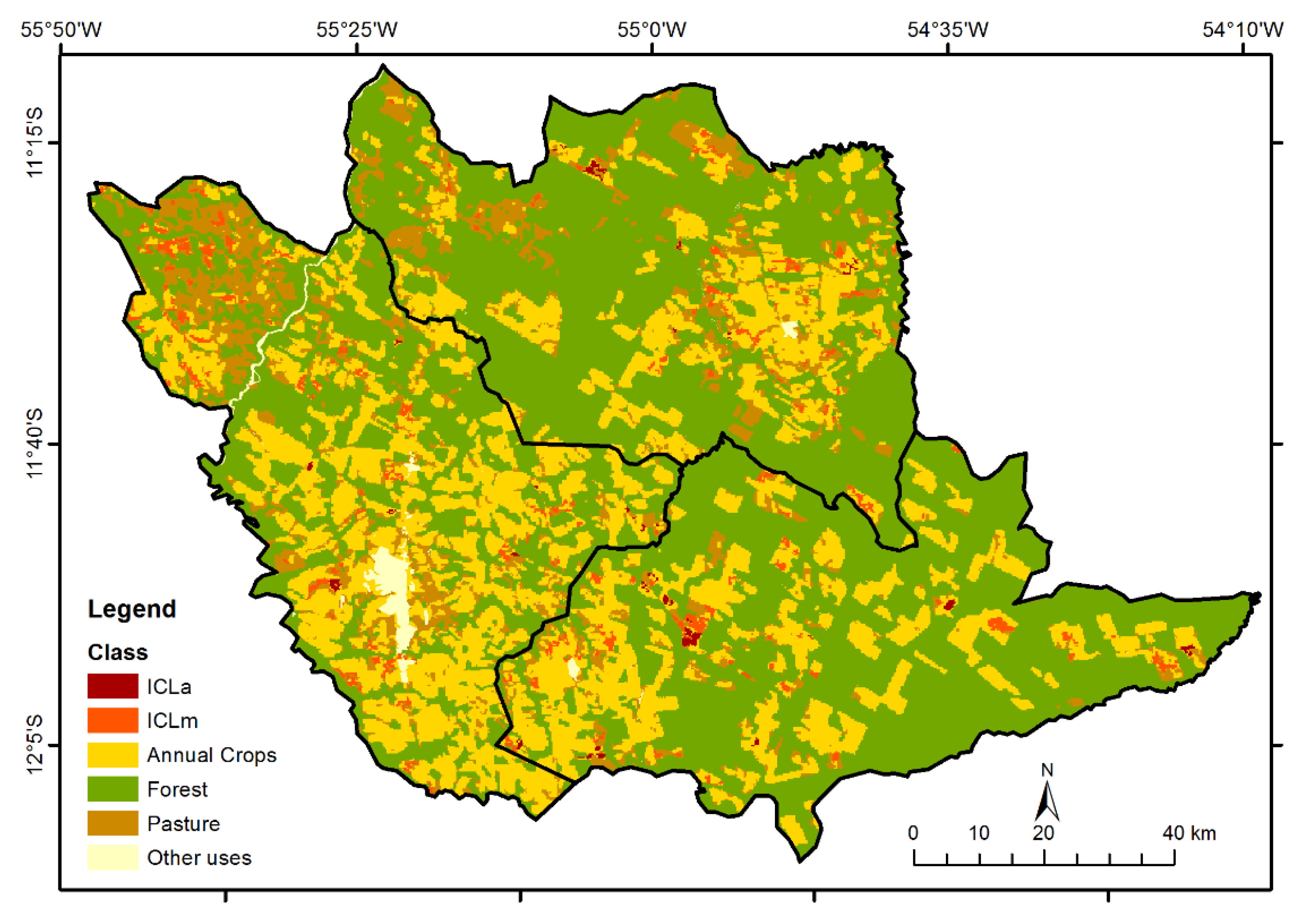
The study area is located in the Sinop, Cláudia, and Santa Carmém municipalities in the Mato Grosso state of Central-Western Brazil, shown in Figure 1. Mato Grosso is among the states that have the largest ICL areas in Brazil [10,17]. Since 2001, intensification in land use has occurred in this region, moving from low-production pasture for cattle ranching to crop production or higher livestock production [38].

In order to understand the distribution and arrangements of ICL systems in the study area, three fieldwork campaigns were conducted. We visited properties that had adopted ICL systems and attended technical meetings at research institutes in order to understand the integration of grain and livestock production in the region. We gathered information about land management, historical land use, and ICL systems.

In addition, to develop and understand the production systems, ground truth information of ICL systems, crops (summer and winter crops), pasture, forest, and other land-use types were collected for the classification framework during the fieldwork campaigns. Information gathered in the first (April 2016) and second (December 2016) field campaigns was used for training the classifier and validation, while information collected from the third (June 2017) campaign was used only for validation.

2.2. MODIS Data

We chose to use the Enhanced Vegetation Index (EVI) product of the MODIS/Terra sensor as it had images recorded throughout the study period and adequate time resolution for seasonal agricultural identification [39,40,41]. Among the MODIS products available, we selected EVI from MOD13Q1, with a 16-day composition and 250 m spatial resolution [42]. Despite the absence of a consensus regarding the best vegetation index for classification [43,44,45], an EVI time-series is more sensitive for high biomass than the NDVI and had been used in previous studies for the temporal characterization and identification of pasture and crop [24,46].

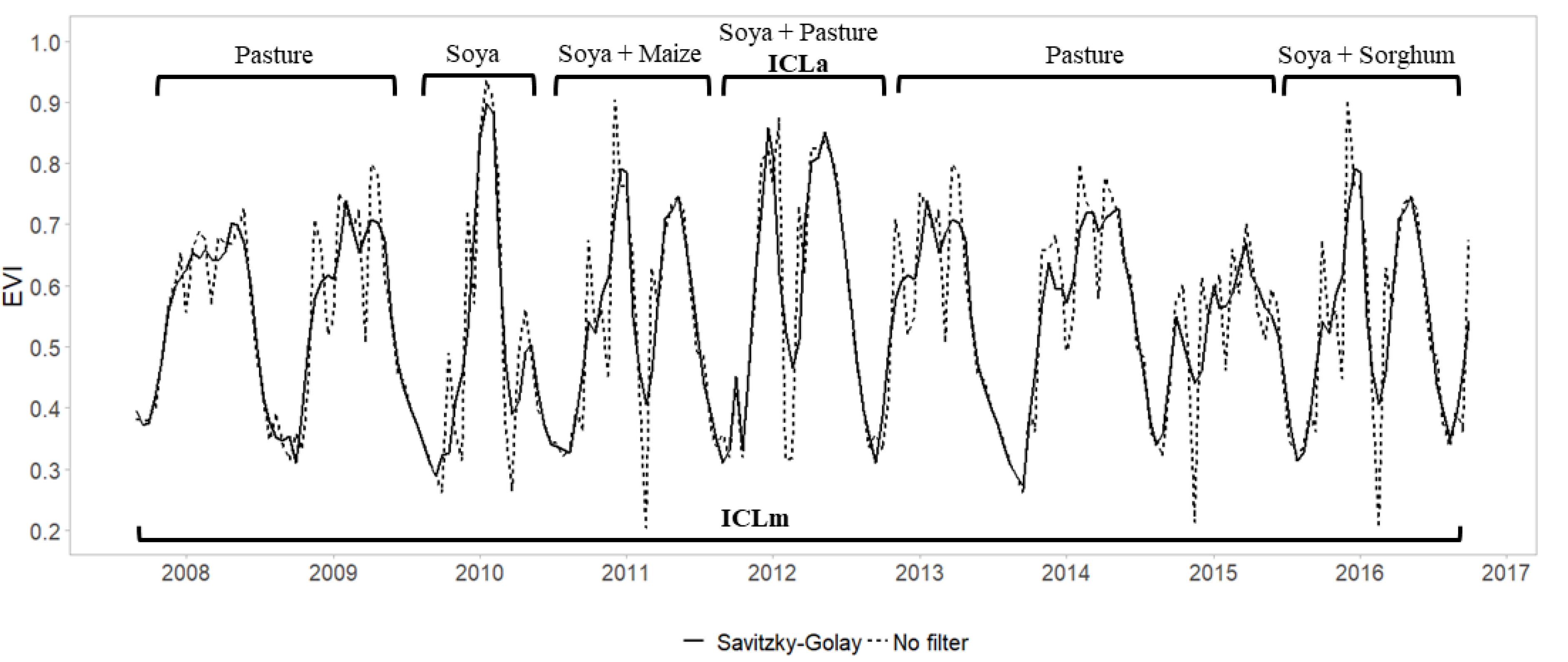
In the ICL classification framework, we used a total of 210 EVI images, from 31 June 2007 to 31 September 2016. The Savitzky–Golay filter was applied to reduce the time-series noise across all periods [47], as shown in Figure 2.

2.3. Field Data

Two types of in situ data were collected across the study area. The first type of ground truth was the history of agricultural practices for individual fields. The focus was to record the location and years where ICLa and ICLm systems occurred. A data acquisition protocol in which farmers/farm managers participated in an interview was established. The participants indicated the property fields by drawing polygons over a Landsat 8 OLI image and described the previous year’s land use in each area. If at least one pixel from MODIS-250 m fitted inside the polygon, a point in the region was created with an unmixed MODIS-250 m pixel. Otherwise, the polygon and the field information was discarded. Thus, during the three fieldwork campaigns, 185 fields in 22 properties were recorded and validated. In the first fieldwork campaign, the field locations were indicated by local researchers and, in the second and third campaigns, the randomly selected points in the classification validation step guided the field visits.

The second type of ground truth was collected in the first fieldwork campaign (April 2016). It was conducted by local field observation for double-crop, single-crop, pasture, and forest. With a Geographic Information System software, Global Positioning System information, Landsat 8 OLI image, and MODIS-250 m pixel grid, fields were visited, and the points were recorded in the center of a homogeneous field which size fitted in one unmixed MODIS 250 m pixel. As the campaign was in April, it was possible to differentiate between single- and double-crop by the observation of winter crops or fallow in crop areas. In total, 280 points were recorded, see

Table 1. Number of field data/points collected by interviews and field observation, for 2016.

Class	Interview	Field Observation	Total
ICLa	55	0	55
ICLm	69	0	69
Single Crop	0	41	41
Double Crop	33	198	231
Pasture	28	9	37
Forest	0	32	32
Total	185	280	465

.

From the field points, ten points were selected for each class, creating the training data set. The selection of training data set points for ICLa, ICLm, Double-Crop (DC), and Pasture, were from the interview data. The rest of the points were allocated in the test data set.

2.4. TWDTW Method

We selected a Time-Weighted Dynamic Time Warping (TWDTW) method for time-series identification [29]. This method is an adaptation of the Dynamic Time Warping (DTW) method, and the R software in the “dtwSat” package were used. Bagnall et al. [48] studied time-series classification and reported that DTW-based methods were among the best performing time-series classification methods. The DTW method involves the comparison of two time-series and subsequent generation of a measure of the dissimilarity, in which lower values indicate a greater similarity in the time-series temporal behavior. However, the DTW method is sensitive to temporal seasonality. In the TWDTW method, Maus et al. [29], adapted the DTW method to find the optimal time-alignment and then generate a measure of dissimilarity (TWDTW distance). Time variations occur in phenological cycles of natural or planted vegetation.

In land-use classification, the identification of time-series was accomplished by defining temporal patterns of land-use classes and generating TWDTW distances through the comparison of temporal patterns with the time-series for each pixel. Each pixel was classified using the temporal pattern with the lowest TWDTW distance, k-Nearest Neighbor where k = 1. The classification method was sufficiently robust to classify single-crops, double-crops, forest, pasture, and certain winter crops using an EVI/MODIS time-series over several years [29,49].

The temporal patterns definition for TWDTW distance generation was created from training samples obtained in the field campaigns. For each class created, the EVI time-series from the training samples were grouped and the Generalized Additive Models (GAM) time-series filter was applied, generating one temporal pattern for each class. The GAM time-series filter was chosen as it was able to generate one time-series from a data set and could be successfully applied to remote sensing data [29,50].

2.5. Classification

The classification framework was designed to detect the two ICL systems, ICLa and ICLm, in the study area of 2016. The ICLa systems had detectable characteristics in one year (crop and pasture in the same agricultural year), requiring classification only for the 2016 agricultural year (September 2015 up to August 2016). The ICLm systems present multi-year characteristics, and for this reason, classification was necessary for each year between 2008 and 2016, as shown in Figure 2.

The following thematic classes were established for all classification processes: Forest, Pasture, SC, DC, ICLa, and ICLm. During the phases of classification, described below, the thematic classes may have been grouped or divided into subclasses to achieve better ICL differentiation, see

Table 2. Description of land cover classes.

Class	Description
ICLa	Integrated crop-livestock in succession in the same area and year
ICLm	Integrated crop-livestock in rotation or succession in the same area and in different years
SC	Exclusive summer crop in a season
DC	Summer and winter crops in a season
Pasture	Natural or planted pasture areas
Forest	Natural or planted forest areas

.

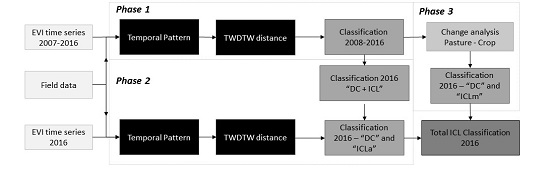
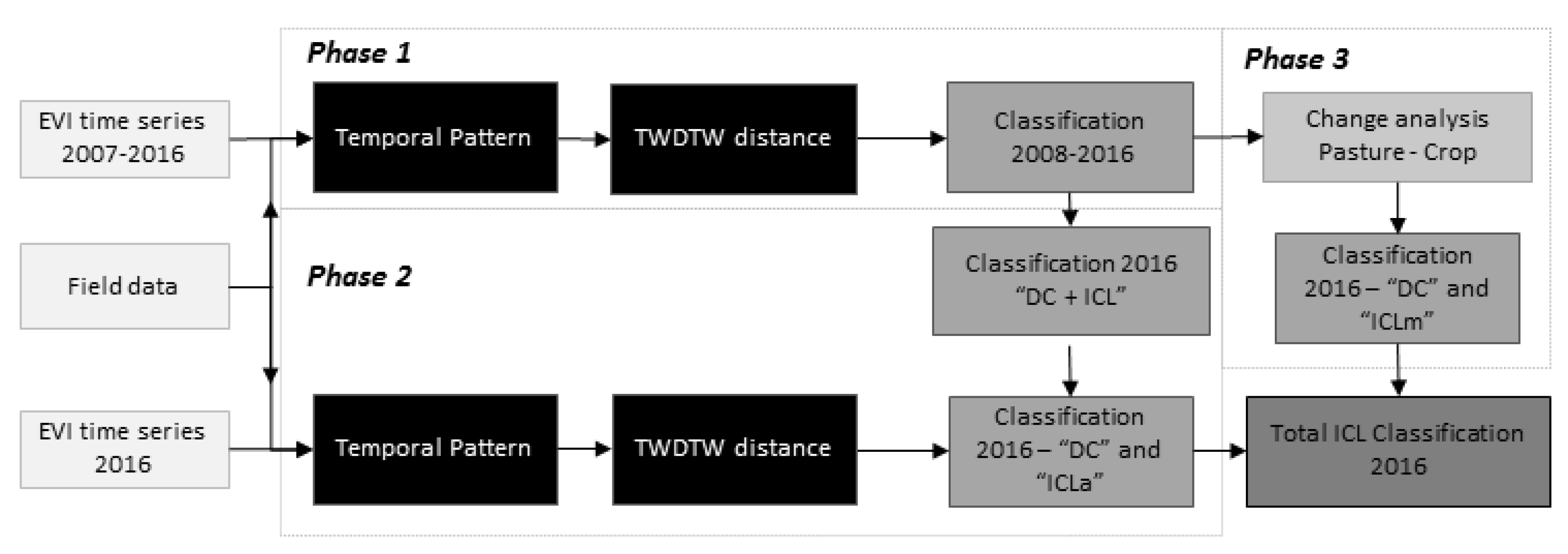
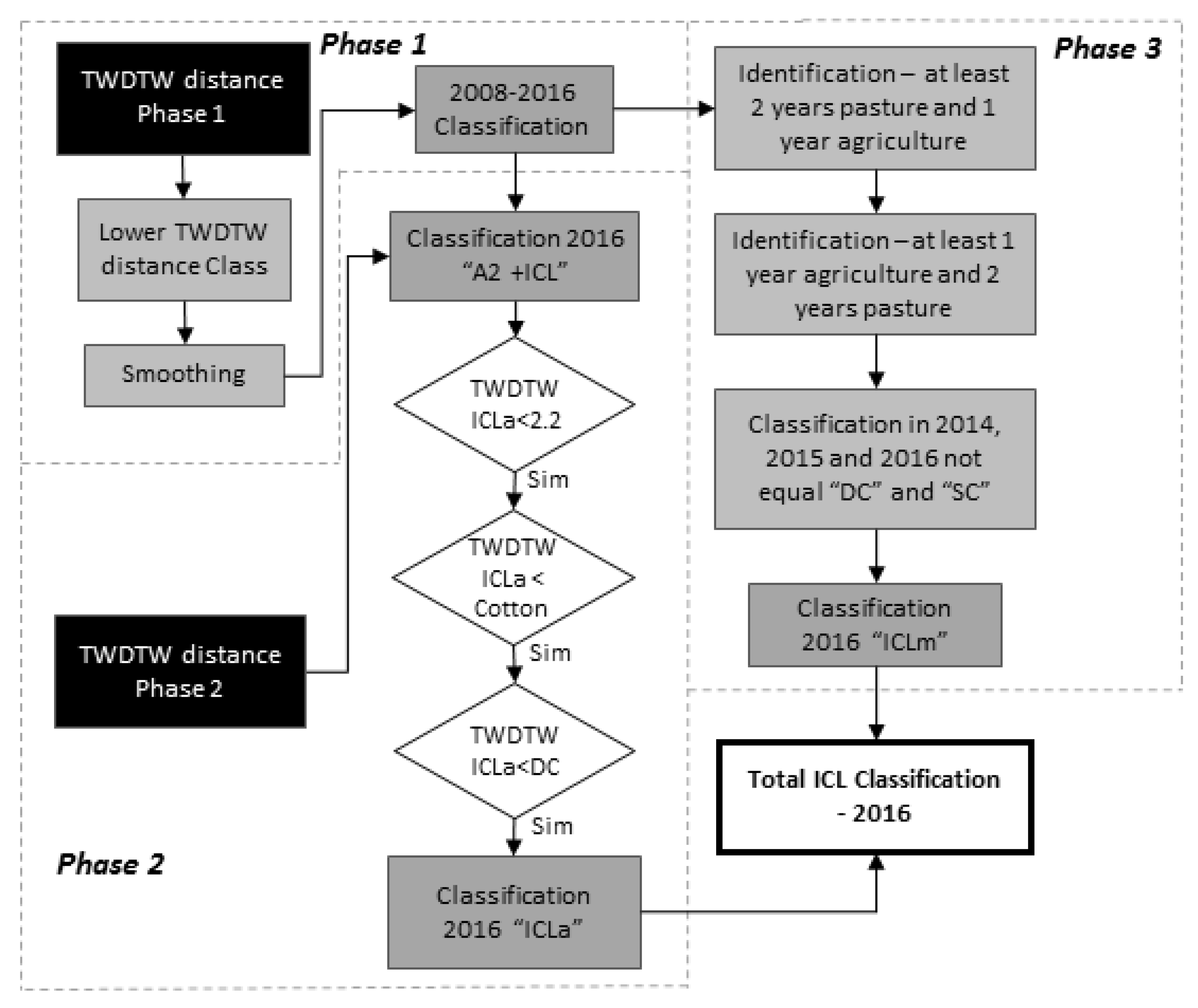
The classification of ICL areas occurred in three phases, as shown in Figure 3. The first corresponded to the classification from 2008 to 2016 of Forest, Pasture, SC, and DC classes, using a temporal period of one agricultural year (September to August). In the second phase, ICLa was identified in a new period of analysis (June to August). In the third phase, an ICLm-class was identified through the land-use change analysis, based on Phase 1 classification. Based on the “Terrclass 2014 project” urban areas, bodies of water, and mining areas were grouped in the class, Others [19].

In the previous analysis, ICLa and DC classification was tested in one step using the annual pattern, which resulted in a great misclassification among these two classes. Therefore, we decided to group all the crops for the two seasons (summer and winter crops) in one class in the first classification phase, and then classify DC and ICLa in the second classification phase. This approach was taken in other studies, where the two-seasons classes were classified separately [24,37,40,46].

2.5.1. Phase 1

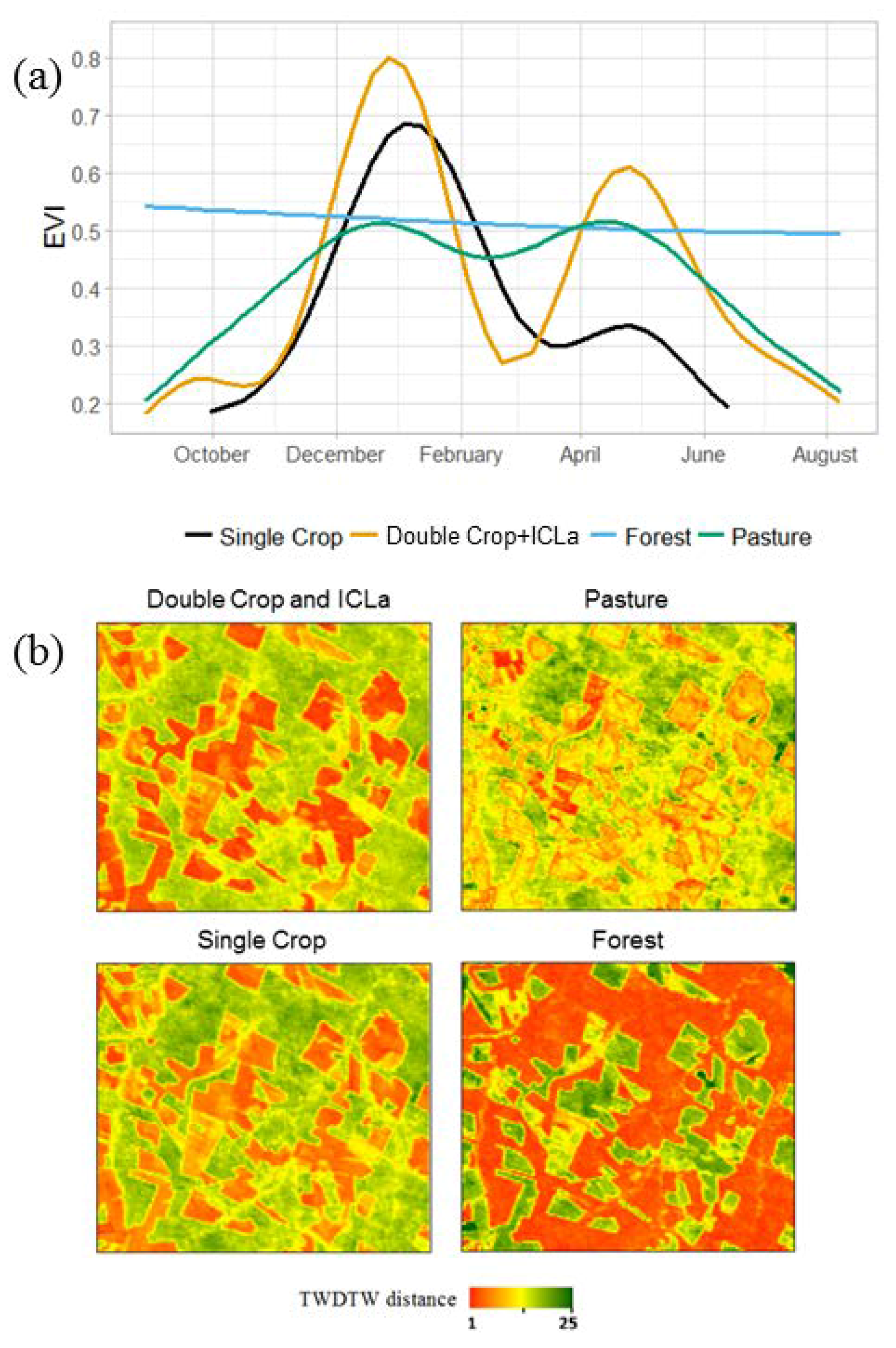
In this step, the classes, Forest, Pasture, SC, and DC + ICLa were classified from 2008 to 2016. The class, DC + ICLa was created by grouping classes, DC and ICLa as they have similar EVI temporal patterns, as shown in Figure 2. In both cases, cultivation of summer crops (usually soya) and winter cultivation (grains for DC and pasture for ICLa) occur, generating a similar annual pattern of vegetation index.

The annual temporal pattern for the classes, as shown in Figure 4a, was determined from the training data collected in the field campaigns. The TWDTW distance was calculated for each class from 2008 until 2016, as shown in Figure 4b. By comparison at the pixel level, the class with the lowest value of TWDTW distance was assigned to the pixel.

2.5.2. Phase 2

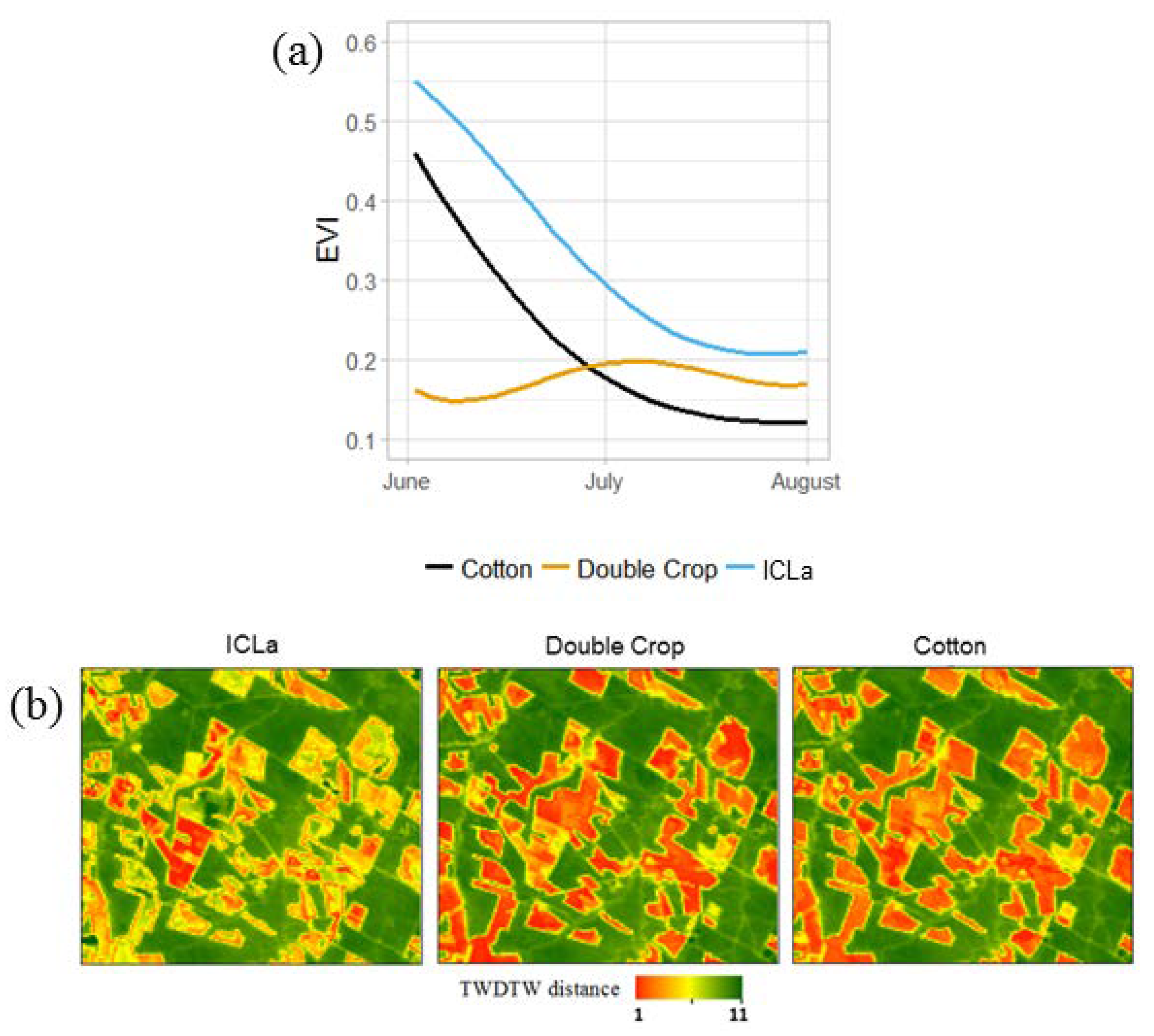
In Phase 2, the areas classified as DC + ICLa in 2016 were separated into DC and ICLa. The winter crop season (June to August) was defined as the period of analysis. After the first tests with TWDTW distance for DC and ICLa separation, the misclassification of cotton cultivation areas as ICLa was observed. Therefore, another class, Cotton, was created at this stage and later reincorporated into DC. Based on field training samples, the temporal patterns for the three classes in this stage (ICLa, Cotton, and DC) were established, and the TWDTW distances for each pattern were generated, see Figure 5.

In the areas classified as DC + ICLa in Phase 1 for the year 2016, the TWDTW distances for the three thematic classes were compared. An area was considered to belong to the class ICLa when the TWDTW distance of ICLa was lower than 2.2, and was the smallest among the other two classes (DC and Cotton), see Figure 6. The definition of values lower than 2.2 occurred based on classification tests. Areas classified as DC + ICLa in Phase 1 and not classified as ICLa in Phase 2 were considered to belong to DC.

2.5.3. Phase 3

In order to detect areas where ICLm occurred as either rotational systems or pasture reform with crop integration, we analyzed changes in the land-use classification between crops and pasture, during 2008–2016.

To be classified as ICLm, pixels were required to have had at least twice the land-use changes–Pasture-Crop (DC or SC), Pasture or Crop (DC or SC), or Pasture-Crop (DC or SC). At least two consecutive years of pasture permanence were also required to avoid including areas that were mistakenly classified as pasture areas in Phase 1. Further, to exclude areas of recent conversion to crop in ICLm, areas classified as crop (SC or DC) since 2014 were not regarded as ICLm, as shown in Figure 6. The classification for the final year, 2016, was evaluated by merging the results generated in Phases 2 and 3. If the same pixel was classified as ICLa and ICLm, the pixel was classified as ICLa.

2.6. Classification Validation

We validated the ICL classification and Phase 1 classification in two different manners; on randomly selected control points and on field data. This was necessary because our field data does not cover the entirety of the study area and is limited to the 2016 classification. The ICL ground truth is difficult to record; therefore an interview protocol is necessary. The randomly selected control points approach made the validation of all study areas over all time periods in Phase 1 possible.

2.6.1. Validation of the MODIS Classification on Randomly Selected Control Points

Phase 1 validation was carried out through analysis of 400 randomly distributed pixels for each year from 2008 to 2016, generating the confusion matrix. The reference for each validation pixel was obtained based on the EVI time-series interpretation. For 2016 classification, 52 points from the test data set were used for validation.

For ICL classification validation, 114 stratified pixels were generated randomly within the area classified as ICL, and 86 stratified pixels were generated randomly outside this area. Pixels in areas classified as ICLa were validated with a visit to the area to collect land-use information. This was necessary, as areas of ICLa, Cotton, and DC are not clearly distinguishable using only the visual interpretation of EVI time-series. For pixels in ICLm areas and outside the ICL areas, verification was based on an EVI time-series visual interpretation and the conditions used in the Phase 3 classification. Visits were made for collecting information on the land-use history of 20 ICLm and five double-crop areas.

2.6.2. Validation of the MODIS Classification on Field Data

The validation of field data was performed for ICL and Phase 1 classification for the year 2016, using all 405 points of the test data set. For Phase 1 2016 classification, a test data set was reordered for the four classes, DC + ICLa, SC, Pasture, and Forest. For ICL classification, the ICL classes merge into one class with non-ICL classes in another.

3. Results

3.1. Validation of the MODIS Classification on Randomly Selected Control Points

In Phase 1, the classifications for DC + ICLa, SC, Pasture, and Forest over the time range of 2008–2016 were generated, as shown in Figure 7. By analyzing the confusion matrix of the Phase 1 classification on randomly selected control points, shown in

Table 3. Confusion matrices and accuracy statistics for Phase 1 classification, validation on randomly selected control points. Note: P, pasture; F, forest; O, other uses; UA, user´s accuracy; PA, producer´s accuracy; OA, overall accuracy.

2008	Reference								2009	Reference
Map	DC + ICL	SC	P	F	O	Total	UA	PA	DC + ICL	SC	P	F	O	Total	UA	PA
DC + ICL	52	8	2	0	1	63	0.83	0.88	55	5	2	1	0	63	0.87	0.73
SC	6	31	8	4	0	49	0.63	0.76	6	24	8	2	0	40	0.60	0.71
P	5	10	42	2	0	59	0.71	0.84	13	3	40	1	2	59	0.68	0.69
F	1	0	10	210	0	221	0.95	0.97	0	2	8	223	0	233	0.96	0.98
O	0	0	0	1	7	8	0.88	0.75	1	0	0	0	4	5	0.80	0.67
Total	64	49	62	217	8		OA:	0.86	75	34	58	227	6		OA:	0.87
2010	Reference								2011	Reference
Map	DC + ICL	SC	P	F	O	Total	UA	PA	DC + ICL	SC	P	F	O	Total	UA	PA
DC + ICL	43	12	5	2	0	62	0.69	0.75	40	14	4	6	0	64	0.63	0.74
SC	4	41	2	0	0	47	0.87	0.68	1	35	3	1	0	40	0.88	0.61
P	9	5	40	8	0	62	0.65	0.83	6	7	34	1	0	48	0.71	0.71
F	1	2	1	220	0	224	0.98	0.96	6	1	7	229	0	243	0.94	0.97
O	0	0	0	0	5	5	1.00	1.00	1	0	0	0	4	5	0.80	1.00
Total	57	60	48	230	5		OA:	0.87	54	57	48	237	4		OA:	0.86
2012	Reference								2013	Reference
Map	DC + ICL	SC	P	F	O	Total	UA	PA	DC + ICL	SC	P	F	O	Total	UA	PA
DC + ICL	49	3	3	2	0	57	0.86	0.71	64	3	5	3	0	75	0.85	0.77
SC	5	20	4	3	0	32	0.63	0.67	11	28	2	2	0	43	0.65	0.78
P	14	3	52	2	0	71	0.73	0.84	6	3	37	2	0	48	0.77	0.76
F	1	4	2	225	2	234	0.96	0.97	2	2	5	219	0	228	0.96	0.96
O	0	0	1	0	5	6	0.83	0.71	0	0	0	2	4	6	0.67	1.00
Total	69	30	62	232	7		OA:	0.88	83	36	49	228	4		OA:	0.88
2014	Reference								2015	Reference
Map	DC + ICL	SC	P	F	O	Total	UA	PA	DC + ICL	SC	P	F	O	Total	UA	PA
DC + ICL	52	7	8	0	0	67	0.87	0.75	66	3	3	4	1	77	0.86	0.81
SC	5	27	5	3	1	41	0.71	0.71	10	22	4	0	0	36	0.61	0.76
P	10	4	36	4	0	54	0.81	0.72	3	3	39	6	0	51	0.76	0.80
F	1	0	1	229	1	232	0.99	0.97	2	1	3	226	0	232	0.97	0.95
O	1	0	0	0	5	6	1.00	0.71	0	0	0	1	3	4	0.75	0.75
Total	69	38	50	236	7		OA:	0.87	81	29	49	237	4		OA:	0.86
2016	Reference
Map	DC + ICL	SC	P	F	O	Total	UA	PA
DC + ICL	58	6	2	1	0	67	0.87	0.88
SC	4	32	6	2	1	45	0.71	0.76
P	3	4	46	4	0	57	0.81	0.84
F	1	0	1	222	1	225	0.99	0.97
O	0	0	0	0	6	6	1.00	0.75
Total	66	42	55	229	8		OA:	0.91

, it was found that the overall classification accuracy varied between 86–91%. The crop classes, DC + ICLa and SC, presented a user´s accuracy (UA) between 0.60–0.88, and a producer´s accuracy (PA) between 0.61–0.87. The higher amount of errors observed for SC were in the DC + ICLa and Pasture, and for DC + ICLa, were in the SC and Pasture classes. Apart from the year 2016, misclassification within DC + ICLa and SC did not influence the ICLm classification. This is because, in the analysis on conversion between crop and pasture in Phase 3, crop classes were grouped. The Pasture class had a UA of 0.65–0.81 and a PA of 0.68–0.84, and errors mainly occurred in classes, SC and Forest. Forest had the largest separation from the other classes with a UA and PA ranging from 0.94–0.99. The classification of DC + ICLa for the year 2016 was made based on the ICLa identification and because the highest UA and PA values, 0.87 and 0.88, respectively, were recorded in this year.

Using the proposed ICL classification framework and validation on randomly selected control points, an overall accuracy of 86% was achieved, as shown in

Table 4. Confusion matrices and accuracy statistics for integrated crop-livestock classification, validation on randomly selected control points.

	Reference
Map	ICL	Others	Total	UA	PA
ICL	91	6	97	0.94	0.80
Others	23	80	103	0.78	0.93
Total	114	86		OA:	0.86

. The UA and PA were 0.80 and 0.94, respectively. Evaluation of the ICL-class classifications, ICLa and ICLm, showed that the crop classes (SC and DC) generated the greatest errors in Phases 1 and 2 of the classification, see

Table 5. Integrated crop–livestock classification errors origins.

Errors	ICLa	ICLm
	%
Classification Phase 1—pasture inclusion error	8	32
Classification Phase 1—SC or DC inclusion error	4	40
Classification Phase 1—other classes inclusion error	1	0
Classification Phase 2—DC inclusion or omission error	6	-
Classification Phase 2—Cotton inclusion error	9	-

. For the ICLa class, the greatest errors occurred in the differentiation of the targets in Phase 2, with difficulty in the separation of ICLa and Cotton. As shown in Figure 5, these two classes had a similar temporal pattern. The highest misclassification errors for ICLm arose when differentiating between Pasture and SC. This led to errors in Phase 3 of the classification as the detection of a land-use change for ICLm generation was compromised. Errors in differentiating between SC and DC occurred in the year 2016, due to a long period of drought during the winter harvest season. However, such errors did not affect the classification of ICL areas significantly.

3.2. Validation of the MODIS Classification on Field Data

The confusion matrix generated from the classification validation on field data for the Phase 1 2016 classification had an accuracy of 0.93, see

Table 6. Confusion matrices and accuracy statistics for Phase 1 classification, validation on field data.

2016	Reference
Map	DC + ICL	SC	P	F	Total	UA	PA
DC + ICL	273	2	7	0	282	0.97	0.94
SC	7	26	0	0	33	0.79	0.84
P	9	3	55	0	67	0.82	0.87
F	0	0	1	22	23	0.96	1.00
Total	289	31	63	22		OA:	0.93

. The classes, DC + ICLa, Pasture, and SC presented a UA between 0.79–0.97 and PA between 0.84–0.94. A larger quantity of errors was found in the misclassification of DC + ICLa and Pasture, and DC + ICLa and SC. The ICL classification for the year 2016, achieved an overall accuracy of 92%, as shown in

Table 7. Confusion matrices and accuracy statistics for integrated crop-livestock classification, validation on field data.

	Reference
Map	ICL	Others	Total	UA	PA
ICL	89	9	98	0.91	0.86
Others	15	282	297	0.95	0.94
Total	104	301		OA:	0.92

. The UA and PA were 0.80 and 0.94, respectively.

3.3. Integrated Crop–Livestock Systems Area

The ICL area in 2016 was 219.18 km², see

Table 8. Classification area, percentage of total agricultural areas and percentage of pasture area.

	Area (km2)	Agriculture	Pasture
Class		Area (%)	Area (%)
ICL	219.18	5	15
ICLa	28.28
ICLm	190.90
Crop	3293.99	69	-
Pasture	1241.17	26	85
Forest	6817.76	-	-

, with ICLa and ICLm areas accounting for 28.28 km² and 190.90 km², respectively. Multi-year systems (ICLm) accounted for 87% of the ICL areas. The area covered by forests is the largest in this region, followed by agriculture and pasture. The ICL systems represented 5% of the total agricultural area found within the study area. If only the pasture is considered, the ICL areas represent 15% of the total area. Indicating that a significant number of livestock producers in the region intensified production by using integrated systems.

4. Discussion and Conclusions

The framework presented herein provided a good accuracy overall in land-use classification and ICL classification, shown in Figure 8. The largest errors for the classes ICLm and ICLa, were distinguishing cotton cultivation and the misclassification between pasture and crop, respectively. The classification techniques proved to be efficient for the characteristics of the land uses in the region. The ICL systems made up 5% of the total agricultural area and 15% of the total pasture area in the study area.

The proposed framework could detect ICL areas within the Sinop, Mato Grosso region. The detection of ICL areas in other regions of Mato Grosso or Brazil will require methodological adjustments due to the possible presence of other land uses, such as sugarcane, natural pastures, and double-crop combinations. However, in regions with the exclusive presence of forest, grains, pasture, and similar ICL systems, only a few adjustments related to the locality may be necessary, such as different periods for establishing the EVI temporal patterns and the creation of new classes in classification Phases 1 and 2.

The overall ICL classification accuracies, in the two validations, were similar to those reported by previous studies that classified summer and winter crops in Mato Grosso using a MODIS vegetation index. Using MODIS/NDVI, Chen et al. [40] classified six crop arrangements; the soya-pasture (ICLm) class had a UA of 0.81 and PA of 0.74. Maus et al. [29] demonstrated the functionality of the TWDTW method for property-scale classification with an overall accuracy of 90%. The classification by Arvor et al. [46] was in two phases; first, the land uses of Cerrado, forest, agriculture, and pasture in the state of Mato Grosso, obtaining an accuracy rate of 86%; second, five crop arrangements obtaining an accuracy rate of 74%.

The most difficult step in this study was the validation step. The reference data obtained from the collected field information was fundamental for validating the accuracy of the classification. However, in ICL areas, the process for obtaining reference information was more complex. This is because, in most cases, it was not possible to determine whether ICL systems were adopted with a single visit to the study area; therefore, either more than one visit was required during the study period or it was necessary to determine the land-use history by interviewing the landowners.

Despite the differences in the two validation methods, the results for the Phase 1 2016 classification did not have large differences and obtained similar values of UA and PA. For ICL classification the validation on field data had a higher accuracy and consequently, more accurate UA and PA values.

The choice of MODIS/Terra in this study was due to the temporal resolution and images available from 2007 to 2016. However, satellite-derived products, such as Landsat-8 OLI, Sentinel-2A, and Sentinel-2B are not sufficiently long-lasting to cover an ICL period of analysis. In the next few years, there is the potential for integrated systems to use these products individually or with fusion techniques, as several studies have shown good results for mapping and monitoring agriculture [20,37,51,52]. Despite the different characteristics of the products, a united source of Landsat-8 and Sentinel-2 data can provide 10–30 m information and produce more frequent observations for monitoring [20]. The TWDTW method had certain applications with Landsat-8 OLI and Sentinel-2 products [37,49,53]. The exploration of the TWDTW method with other classification techniques offers an opportunity for future studies. Belgiu and Csillik [49] showed good results when they combined object-oriented classification and the TWDTW method.

References

1. Lapola, D.M.; Martinelli, L.A.; Peres, C.A.; Ometto, J.P.H.B.; Ferreira, M.E.; Nobre, C.A.; Aguiar, A.P.D.; Bustamante, M.M.C.; Cardoso, M.F.; Costa, M.H.; et al. Pervasive transition of the Brazilian land-use system. Nat. Clim. Chang. 2013, 4, 27–35. [Google Scholar] [CrossRef]
2. Strassburg, B.B.N.; Latawiec, A.E.; Barioni, L.G.; Nobre, C.A.; da Silva, V.P.; Valentim, J.F.; Vianna, M.; Assad, E.D. When enough should be enough: Improving the use of current agricultural lands could meet production demands and spare natural habitats in Brazil. Glob. Environ. Chang. 2014, 28, 84–97. [Google Scholar] [CrossRef] [Green Version]
3. Salton, J.C.; Mercante, F.M.; Tomazi, M.; Zanatta, J.A.; Concenço, G.; Silva, W.M.; Retore, M. Integrated crop-livestock system in tropical Brazil: Toward a sustainable production system. Agric. Ecosyst. Environ. 2014, 190, 70–79. [Google Scholar] [CrossRef]
4. Tarawali, S.; Herrero, M.; Descheemaeker, K.; Grings, E.; Blümmel, M. Pathways for sustainable development of mixed crop livestock systems: Taking a livestock and pro-poor approach. Livest. Sci. 2011, 139, 11–21. [Google Scholar] [CrossRef]
5. Herrero, M.; Thornton, P.K.; Notenbaert, A.M.; Wood, S.; Msangi, S.; Freeman, H.A.; Bossio, D.; Dixon, J.; Peters, M.; van de Steeg, J.; et al. Smart Investments in Sustainable Food Production: Revising Mixed Crop-Livestock Systems. Science 2010, 327, 821–824. [Google Scholar] [CrossRef] [PubMed]
6. Balbino, L.C.; Barcellos, A.D.O.; Stones, L.F. Landmark: Crop-Livestock-Forest Integration; Embrapa: Brasilia, Brazil, 2011. (In Portuguese) [Google Scholar]
7. Vilela, L.; Martha Junior, G.B.; Motta Macedo, M.C.; Marchao, R.L.; Guimaraes Junior, R.; Pulrolnik, K.; Maciel, G.A. Integrated crop-livestock systems in the Cerrado region. Pesqui. Agropecu. Bras. 2011, 46, 1127–1138. [Google Scholar] [CrossRef]
8. Landers, J.N. Tropical Crop-Livestock Systems in Conservation Agriculture: The Brazilian Experience; Food & Agriculture Organization of the United Nations: Rome, Italy, 2007. [Google Scholar]
9. De Moraes, A.; Carvalho, P.C.D.F.; Anghinoni, I.; Lustosa, S.B.C.; de Andrade, S.E.V.G.; Kunrath, T.R. Integrated crop-livestock systems in the Brazilian subtropics. Eur. J. Agron. 2014, 57, 4–9. [Google Scholar] [CrossRef]
10. Gil, J.; Siebold, M.; Berger, T. Adoption and development of integrated crop-livestock-forestry systems in Mato Grosso, Brazil. Agric. Ecosyst. Environ. 2015, 199, 394–406. [Google Scholar] [CrossRef]
11. Amaral, D.D.D.; Cordeiro, L.A.M.; Galerani, P.R. Sectorial Plan for Mitigation and Adaptation to Climate Change for the Consolidation of a Low Carbon Economy in Agriculture—ABC Plan. Rev. Bras. Geogr. Física 2011, 4, 1266–1274. (In Portuguese) [Google Scholar] [CrossRef]
12. Lange, A.; Cristina, A.; Ferreira, T.; Lemke, A.F.; Buchelt, A.C.; Diana, C.; Luiz, E. Pasture, Silage and Straw in the Crop-Livestock. Rev. Bras. Milho e Sorgo 2013, 12, 293–306. [Google Scholar] [CrossRef]
13. Franzluebbers, A.J.; Sawchik, J.; Taboada, M.A. Agronomic and environmental impacts of pasture-crop rotations in temperate North and South America. Agric. Ecosyst. Environ. 2014, 190, 18–26. [Google Scholar] [CrossRef]
14. Carvalho, J.L.N.; Raucci, G.S.; Cerri, C.E.P.; Bernoux, M.; Feigl, B.J.; Wruck, F.J.; Cerri, C.C. Impact of pasture, agriculture and crop-livestock systems on soil C stocks in Brazil. Soil Tillage Res. 2010, 110, 175–186. [Google Scholar] [CrossRef]
15. De Oliveira, P.; Freitas, R.J.; Kluthcouski, J.; Ribeiro, A.A.; Adriano, L.; Cordeiro, M.; Teixeira, L.P.; Augusto, R.; Castro, D.; Vilela, L.; et al. Evolução de Sistemas de Integração Lavoura-Pecuária-Floresta (iLPF): Estudo de caso da Fazenda Santa Brígida, Ipameri, GO; Embrapa Arroz e Feijão: Planaltina, Brazil, 2013; pp. 1–51. [Google Scholar]
16. Latawiec, A.E.; Strassburg, B.B.N.; Valentim, J.F.; Ramos, F.; Alves-Pinto, H.N. Intensification of cattle ranching production systems: Socioeconomic and environmental synergies and risks in Brazil. Animal 2014, 8, 1255–1263. [Google Scholar] [CrossRef] [PubMed]
17. Embrapa ILPF em número. ILPF em Números; Embrapa Agrossilvipastoril: Brasília, Brasil, 2016. [Google Scholar]
18. Sahajpal, R.; Zhang, X.; Izaurralde, R.C.; Gelfand, I.; Hurtt, G.C. Identifying representative crop rotation patterns and grassland loss in the US Western Corn Belt. Comput. Electron. Agric. 2014, 108, 173–182. [Google Scholar] [CrossRef]
19. De Almeida, C.A.; Coutinho, A.C.; Esquerdo, J.C.D.M.; Adami, M.; Venturieri, A.; Diniz, C.G.; Dessay, N.; Durieux, L.; Gomes, A.R. High spatial resolution land use and land cover mapping of the Brazilian Legal Amazon in 2008 using Landsat-5/TM and MODIS data. Acta Amaz. 2016, 46, 291–302. [Google Scholar] [CrossRef] [Green Version]
20. Jakimow, B.; Griffiths, P.; van der Linden, S.; Hostert, P. Mapping pasture management in the Brazilian Amazon from dense Landsat time series. Remote Sens. Environ. 2018, 205, 453–468. [Google Scholar] [CrossRef]
21. García-Mora, T.J.; Mas, J.-F.; Hinkley, E.A. Land cover mapping applications with MODIS: A literature review. Int. J. Digit. Earth 2012, 5, 63–87. [Google Scholar] [CrossRef]
22. Tatsumi, K.; Yamashiki, Y.; Canales Torres, M.A.; Taipe, C.L.R. Crop classification of upland fields using Random forest of time-series Landsat 7 ETM+ data. Comput. Electron. Agric. 2015, 115, 171–179. [Google Scholar] [CrossRef]
23. Schwieder, M.; Leitão, P.J.; da Cunha Bustamante, M.M.; Ferreira, L.G.; Rabe, A.; Hostert, P. Mapping Brazilian savanna vegetation gradients with Landsat time series. Int. J. Appl. Earth Obs. Geoinform. 2016, 52, 361–370. [Google Scholar] [CrossRef]
24. Brown, J.C.; Kastens, J.H.; Coutinho, A.C.; de Castro Victoria, D.; Bishop, C.R. Classifying multiyear agricultural land use data from Mato Grosso using time-series MODIS vegetation index data. Remote Sens. Environ. 2013, 130, 39–50. [Google Scholar] [CrossRef]
25. Le Maire, G.; Dupuy, S.; Nouvellon, Y.; Loos, R.A.; Hakamada, R. Mapping short-rotation plantations at regional scale using MODIS time series: Case of eucalypt plantations in Brazil. Remote Sens. Environ. 2014, 152, 136–149. [Google Scholar] [CrossRef]
26. Phompila, C.; Lewis, M.; Ostendorf, B.; Clarke, K. MODIS EVI and LST Temporal Response for Discrimination of Tropical Land Covers. Remote Sens. 2015, 7, 6026–6040. [Google Scholar] [CrossRef] [Green Version]
27. Shahriar Pervez, M.; Budde, M.; Rowland, J. Mapping irrigated areas in Afghanistan over the past decade using MODIS NDVI. Remote Sens. Environ. 2014, 149, 155–165. [Google Scholar] [CrossRef] [Green Version]
28. Arvor, D.; Meirelles, M.; Dubreuil, V.; Bégué, A.; Shimabukuro, Y.E. Analyzing the agricultural transition in Mato Grosso, Brazil, using satellite-derived indices. Appl. Geogr. 2012, 32, 702–713. [Google Scholar] [CrossRef] [Green Version]
29. Maus, V.; Câmara, G.; Cartaxo, R.; Sanchez, A.; Ramos, F.M.; Ribeiro, G.Q. A Time-Weighted Dynamic Time Warping method for land use and land cover mapping. IEEE J. Sel. Top. Appl. Earth Obs. Remote Sens. 2015, 9, 3729–3739. [Google Scholar] [CrossRef]
30. Adami, M.; Rudorff, B.F.T.; Freitas, R.M.; Aguiar, D.A.; Sugawara, L.M.; Mello, M.P. Remote Sensing Time Series to Evaluate Direct Land Use Change of Recent Expanded Sugarcane Crop in Brazil. Sustainability 2012, 4, 574–585. [Google Scholar] [CrossRef] [Green Version]
31. Alcantara, C.; Kuemmerle, T.; Prishchepov, A.V.; Radeloff, V.C. Mapping abandoned agriculture with multi-temporal MODIS satellite data. Remote Sens. Environ. 2012, 124, 334–347. [Google Scholar] [CrossRef]
32. Lu, M.; Pebesma, E.; Sanchez, A.; Verbesselt, J. Spatio-temporal change detection from multidimensional arrays: Detecting deforestation from MODIS time series. ISPRS J. Photogramm. Remote Sens. 2016, 117, 227–236. [Google Scholar] [CrossRef]
33. Clark, M.L.; Aide, T.M.; Riner, G. Land change for all municipalities in Latin America and the Caribbean assessed from 250-m MODIS imagery (2001–2010). Remote Sens. Environ. 2012, 126, 84–103. [Google Scholar] [CrossRef]
34. Siachalou, S.; Mallinis, G.; Tsakiri-Strati, M. A hidden markov models approach for crop classification: Linking crop phenology to time series of multi-sensor remote sensing data. Remote Sens. 2015, 7, 3633–3650. [Google Scholar] [CrossRef]
35. Poccard-Chapuis, R.; Navegantes Alves, L.; Grise, M.M.; Bâ, A.; Coulibaly, D.; Ferreira, L.A.; Lecomte, P. Landscape characterization of integrated crop–livestock systems in three case studies of the tropics. Renew. Agric. Food Syst. 2014, 29, 218–229. [Google Scholar] [CrossRef]
36. Shao, Y.; Lunetta, R.S.; Wheeler, B.; Iiames, J.S.; Campbell, J.B. An evaluation of time-series smoothing algorithms for land-cover classifications using MODIS-NDVI multi-temporal data. Remote Sens. Environ. 2016, 174, 258–265. [Google Scholar] [CrossRef]
37. Belgiu, M.; Csillik, O. Sentinel-2 cropland mapping using pixel-based and object-based time-weighted dynamic time warping analysis. Remote Sens. Environ. 2018, 204, 509–523. [Google Scholar] [CrossRef]
38. Cohn, A.S.; Gil, J.; Berger, T.; Pellegrina, H.; Toledo, C. Patterns and processes of pasture to crop conversion in Brazil: Evidence from Mato Grosso State. Land Use Policy 2016, 55, 108–120. [Google Scholar] [CrossRef]
39. Aguiar, D.A.; Mello, M.P.; Nogueira, S.F.; Gonçalves, F.G.; Adami, M.; Theodor Rudorff, B.F. MODIS time series to detect anthropogenic interventions and degradation processes in tropical pasture. Remote Sens. 2017, 9, 73. [Google Scholar] [CrossRef]
40. Chen, Y.; Lu, D.; Moran, E.; Batistella, M.; Dutra, L.V.; Sanches, I.D.; da Silva, R.F.B.; Huang, J.; Luiz, A.J.B.; de Oliveira, M.A.F. Mapping croplands, cropping patterns, and crop types using MODIS time-series data. Int. J. Appl. Earth Obs. Geoinform. 2018, 69, 133–147. [Google Scholar] [CrossRef]
41. Gu, Y.; Brown, J.F.; Verdin, J.P.; Wardlow, B. A five-year analysis of MODIS NDVI and NDWI for grassland drought assessment over the central Great Plains of the United States. Geophys. Res. Lett. 2007, 34, L06407. [Google Scholar] [CrossRef]
42. Huete, A.; Didan, K.; Miura, H.; Rodriguez, E.P.; Gao, X.; Ferreira, L.F. Overview of the radiometric and biopyhsical performance of the MODIS vegetation indices. Remote Sens. Environ. 2002, 83, 195–213. [Google Scholar] [CrossRef]
43. Wang, C.; Jamison, B.E.; Spicci, A.A. Trajectory-based warm season grassland mapping in Missouri prairies with multi-temporal ASTER imagery. Remote Sens. Environ. 2010, 114, 531–539. [Google Scholar] [CrossRef]
44. Wardlow, B.; Egbert, S.; Kastens, J. Analysis of time-series MODIS 250 m vegetation index data for crop classification in the U.S. Central Great Plains. Remote Sens. Environ. 2007, 108, 290–310. [Google Scholar] [CrossRef] [Green Version]
45. Yan, E.; Wang, G.; Lin, H.; Xia, C.; Sun, H. Phenology-based classification of vegetation cover types in Northeast China using MODIS NDVI and EVI time series. Int. J. Remote Sens. 2015, 36, 489–512. [Google Scholar] [CrossRef]
46. Arvor, D.; Jonathan, M.; Meirelles, M.S.P.; Dubreuil, V.; Durieux, L. Classification of MODIS EVI time series for crop mapping in the state of Mato Grosso, Brazil. Int. J. Remote Sens. 2011, 32, 7847–7871. [Google Scholar] [CrossRef]
47. Chen, J.; Jönsson, P.; Tamura, M.; Gu, Z.; Matsushita, B.; Eklundh, L. A simple method for reconstructing a high-quality NDVI time-series data set based on the Savitzky–Golay filter. Remote Sens. Environ. 2004, 91, 332–344. [Google Scholar] [CrossRef]
48. Bagnall, A.; Lines, J.; Bostrom, A.; Large, J.; Keogh, E. The great time series classification bake off: A review and experimental evaluation of recent algorithmic advances. Data Min. Knowl. Discov. 2017, 31, 606–660. [Google Scholar] [CrossRef]
49. Csillik, O.; Belgiu, M. Cropland mapping from Sentinel-2 time series data using object-based image analysis. In Proceedings of the 20th AGILE International Conference on Geographic Information Science Societal Geo-Innovation Celebrating 20 years of GIS Research, Wageningen, The Netherlands, 9–12 May 2017. [Google Scholar]
50. Wood, S.N. Fast stable restricted maximum likelihood and marginal likelihood estimation of semiparametric generalized linear models. J. R. Stat. Soc. Ser. B Stat. Methodol. 2011, 73, 3–36. [Google Scholar] [CrossRef] [Green Version]
51. Parente, L.; Ferreira, L.; Faria, A.; Nogueira, S.; Araújo, F.; Teixeira, L.; Hagen, S. Monitoring the brazilian pasturelands: A new mapping approach based on the landsat 8 spectral and temporal domains. Int. J. Appl. Earth Obs. Geoinf. 2017, 62, 135–143. [Google Scholar] [CrossRef]
52. Bégué, A.; Arvor, D.; Bellon, B.; Betbeder, J.; de Abelleyra, D.; Ferraz, R.P.D.; Lebourgeois, V.; Lelong, C.; Simões, M.; Verón, S.R. Remote sensing and cropping practices: A review. Remote Sens. 2018, 10, 99. [Google Scholar] [CrossRef]
53. Simoes, R.; Pletsch, M.; Santos, L.; Câmara, G.; Maus, V. Satellite Multisensor Spatiotemporal Analysis: A TWDTW preview approach. In Proceedings of the XVII SBSR Brazilian Symposium on Remote Sensing, Santos, Brazil, 28–31 May 2017; pp. 6943–6950. [Google Scholar]
Figure 1. Study area: Sinop, Cláudia, and Santa Carmém municipalities in Northern Mato Grosso, Brazil.
Remotesensing 10 01322 g001
Figure 2. Examples of annual integrated crop-livestock (ICLa) and multi-annual integrated crop-livestock (ICLm) Enhanced Vegetation Index (EVI) temporal behavior, non-filtered, and filtered by Savitzky-Golay method. The brackets highlight land-use changes between crop and pasture across multiple agricultural years, and within an agricultural year, represented by ICLm and ICLa, respectively.
Remotesensing 10 01322 g002
Figure 3. The flowchart of the proposed method for mapping integrated crop-livestock systems. Note: ICL, integrated crop-livestock.
Remotesensing 10 01322 g003
Figure 4. (a) Temporal patterns and (b) TWDTW distance subset for classes in Phase 1. Note: TWDTW, Time-Weighted Dynamic Time Warping.
Remotesensing 10 01322 g004
Figure 5. (a) Temporal patterns and (b) TWDTW distance subset for classes in Phase 2.
Remotesensing 10 01322 g005
Figure 6. The flowchart of the mapping framework for integrated crop-livestock systems, Phase 1–3.
Remotesensing 10 01322 g006
Figure 7. Phase 1 classification for the years 2008–2016.
Remotesensing 10 01322 g007
Figure 8. Integrated crop-livestock classification for 2016.
Remotesensing 10 01322 g008