Article

Classifying the Built-Up Structure of Urban Blocks with Probabilistic Graphical Models and TerraSAR-X Spotlight Imagery

1
GIScience Research Group, Institute of Geography, Heidelberg University, 69120 Heidelberg, Germany
2
Photogrammetrie und Fernerkundung, Technische Universitaet Muenchen, 80333 München, Germany
*
Author to whom correspondence should be addressed.
Current address: Im Neuenheimer Feld 348, 69120 Heidelberg, Germany.
These authors contributed equally to this work.
Remote Sens. 2018, 10(6), 842; https://doi.org/10.3390/rs10060842
Submission received: 25 April 2018 / Revised: 16 May 2018 / Accepted: 22 May 2018 / Published: 28 May 2018
(This article belongs to the Section Remote Sensing Image Processing)

Abstract

:
Up-to-date maps of a city’s urban structure types (USTs) are very important for effective planning, as well as for different studies and applications. We present an approach for the classification of USTs at the level of urban blocks based on high-resolution spaceborne radar imagery. Images obtained at the satellite’s ascending and descending orbits were used for extracting line and polygon features from each block. Most of the attributes considered in the classification concern the geometry of these features, as well as their spatial disposition inside the blocks. Furthermore, assuming the UST classes of neighboring blocks are probabilistically dependent, we explored the framework of probabilistic graphical models and propose different context-based classification models. These models differ with respect to (i) their type, i.e., Markov or conditional random fields, (ii) their parameterization and (iii) the criterion applied for establishing pairwise neighboring relationships between blocks. In our experiments, 1,695 blocks from the city of Munich (Germany) and five representative UST classes were considered. A standard classification performed with the Random Forest algorithm achieved an overall accuracy of nearly 70%. All context-based classifications achieved overall accuracies up to 7% higher than that. The results indicate that denser pairwise block-neighborhood structures lead to better results and that the accuracy improvement is higher when the strength of the contextual influences is proportional to the similarity of the neighboring blocks attributes.

1. Introduction

Developing countries are not the only ones experiencing the expansion and densification of urban areas. Despite their low population growth rates, developed countries, whose urban population is already over 70%, are also facing these issues [1]. In Germany alone, each day, 73 hectares of land on average were converted to urban areas in the period between 2010 and 2013 [2]. Climate discomfort, air and noise pollution, traffic congestion and an increase in the rent prices are some of the consequences that may arise from this process. These and other threats to the citizens’ quality of life may be avoided or mitigated by means of appropriate zoning policies that regulate the spatial distribution of the urban land use. In Germany, the generally adopted synonym for urban land use is the concept Stadtstrukturtypen, or urban structure types (USTs). USTs serve as a common basis for the categorization of the urban surface that guides past, current and future planning and monitoring tasks [3]. More specifically, the up-to-date information on the distribution of a city’s USTs supports the management of water and energy supply, the promotion and management of public health and safety, the preservation of historically- and culturally-significant areas, as well as the efficient allocation of urban equipment. Furthermore, UST zoning serves to encourage economic development while at the same time assuring residential property values by guaranteeing that incompatible uses will be kept apart.
Although USTs are also defined based on socio-economic and functional aspects, most of them are strongly characterized by structural attributes, such as the relative orientation and density of the buildings, as well as by environmental factors, such as the amount, size and types of vegetated and sealed areas. This makes it possible that the production and updating of UST maps be supported by remote sensing image classification, which, in comparison to ground surveys and visual image interpretation, is an automatic, objective, faster and less resource-demanding way to accomplish this task.
Since UST classes are always defined at the level of some spatial aggregate, the vast majority of approaches proposed for classifying USTs based on remote sensing images have considered as elements of analysis either user-defined grid-cells [4,5,6] or some of the city’s administrative parcels, like census tracts [7], urban districts [8] or, most frequently, the city’s urban blocks [9,10,11,12,13]. Being the largest areas surrounded by streets, urban blocks are frequently the spatial unit based on which urban zoning laws are defined and official land use maps are produced. Because of that, studies dedicated to remote sensing-based UST discrimination of German cities have all considered urban blocks as the elementary analysis units. Banzhaf et al. [9] distinguished different USTs from Leipzig based on an object-based image analysis approach and aerial photographs. In a similar work, Voltersen et al. [12] included the height information from a stereoscopic pair of aerial images to support the classification of USTs from Berlin. Walde et al. [14] focused on describing urban blocks in Jena according to the spatial disposition of their land cover features connected by a graph. The approach had been previously tested in Rostock and Erfurt by the same authors [15]. Wurm et al. [16] performed UST classification from the cities of Cologne and Dresden based on high-resolution optical imagery and a digital surface model. They first performed an object-based land cover classification of the scenes and then described the urban blocks according to the structure of their land cover features. Also based on a land cover classification performed based on height information and hyperspectral imagery, Heiden et al. [11] classified urban blocks from Munich according to their predominant UST.

1.1. Descriptive Attributes for Classifying Urban Structure Types

Urban features, e.g., buildings, houses, sealed and vegetated areas, and the urban blocks where these features are located are unique with respect to their shape, size and orientation. Also unique is the spatial disposition of the features inside each block. Thus, no two blocks are ever identical with respect to their built-up structures and shapes. This makes the conception of expressive attributes particularly challenging when performing block-based classification of USTs with remote sensing images. The underlying assumptions are (i) that the blocks belonging to a given UST class have similar built-up structures and (ii) that classes defined mainly by functional and social aspects have typical structural patterns that enable their distinction based on image-derived attributes.
One type of attribute previously used for that aim is texture descriptors. Texture images can be generated and their pixel values aggregated to the block level by first-order statistics (i.e., mean, max., std. deviation, etc.) [17]. Alternatively, the metrics can be computed directly for each block separately [4,18]. Texture metrics are to a certain extent expressive; however, a more human-interpretable and effective approach attempts to formalize the evidence considered by a human interpreter by means of higher-level attributes. These attributes can be of two types, namely composition and disposition attributes.
Composition attributes describe the type, number, relative area (with respect to the block’s area) and geometric properties of the features inside each block, whereas the more complex disposition attributes describe their spatial configuration. In many works, such higher-level attributes are computed after extracting features inside the blocks through a land cover classification procedure [12,19,20,21]. This approach has been adopted in order to perform block-based UST and urban land use classification using multispectral [12,22] and hyperspectral images [11,23], as well as LiDAR data [11,15]. These works assume that their land cover classification is accurate enough so that the composition and disposition attributes derived from it are expressive enough for distinguishing the USTs or land use classes. Indeed, object-based image analysis techniques, which are frequently resorted to in these studies, have proven to be very effective for high-resolution optical image classification in a number of different applications [24,25].
Composition attributes are able to describe the built-up structure of a block only partially. Typical UST classes like perimeter block development, row house development and regular block development [26] can only be properly described and accurately distinguished if disposition attributes are also considered. Simple examples of disposition attributes previously used for parcel-based land use classification are: average nearest distance between buildings [8], minimal distance of the building contour to the closest block boundary [27] and number of buildings with orientation difference between (computed for different angle intervals) [12]. More elaborated disposition attributes were proposed by Vanderhaegen et al. [28]. They produced for each block a certain number of radial and contour profiles and then calculated for each of them different indexes related to the building/non-building alternations, as well as to the lengths of the building and non-building profile segments. Examples of these indexes computed for each profile are: normalized number of building segments, average length of building segments and standard deviation of the length of the building profile segments. Another way of describing the disposition of objects inside a block is by creating a network connecting neighboring features of the same or related types (e.g., same or related land cover class) and then extracting attributes from this network, as performed by Hermosillaa et al. [29] and Walde et al. [14]. Such a network is created usually by defining one node for each feature and then establishing edges between them based, for example, on the criteria of direct adjacency or distance thresholds. Examples of attributes that can be computed from the network include: number of edges connecting objects of the same type, number of edges connecting objects of different types, proportion of edges connecting objects of the same type, mean orientation difference between connected nodes, mean distance between connected nodes, standard deviation of the distance between connected objects of the same type and density of the network. Possibly, one of the reasons for the fact that composition attributes are used more frequently than disposition attributes is that most of the innumerable disposition attributes are not available in object-based image analysis software and require therefore that the user implement their computation.

1.2. Main Assumptions and Contributions of This Paper

The motivation for investigating whether considering each block’s context is expected to increase the UST classification accuracy lies in the assumption that the spatial distribution of the USTs in a particular city is not random. Indeed, urban blocks from the same UST class are frequently found close to each other. Moreover, two UST classes may be related in a way that we expect to find one close to the other. For example, parks may be found more frequently in residential areas than in industrial areas. The assumption that the spatial distribution of USTs is not random can be justified in different ways. Waldo Tobler [30] proposed the first law of geography for which “everything is related to everything else, but near things are more related than distant things”. Indeed, it is somewhat common sense that similar or related things tend to be close to each other, as things close to each other tend to be similar or related. Furthermore, the existence in many cities of urban zoning laws leads to a rational spatial distribution of the USTs aiming to preserve the citizens’ quality of life and to yield a efficient circulation of people and goods. If these assumptions hold, then the context of each block is informative and should be thus considered in the UST classification.
Different from other works that used spaceborne synthetic aperture radar (SAR) and optical imagery for detecting and roughly distinguishing urban areas at the pixel level [31,32,33,34], we attempt to distinguish USTs at the level of urban blocks. For that, spaceborne SAR images obtained at the satellite’s ascending and descending orbits are used. Instead of describing the blocks’ built-up structure based on attributes computed from a previously-performed land cover classification, our block-base UST classification approach is based on attributes related to the geometric characteristics and spatial disposition of lines and polygon features extracted from each block. These features are extracted from the SAR images from both orbits. Furthermore, and most importantly, we investigate to what extent the accuracy of UST classifications can be improved if the context of each block is considered. For that, the powerful and flexible framework of Probabilistic Graphical Models is explored. Different model parameterizations and context definition criteria are proposed and evaluated.

2. Methods

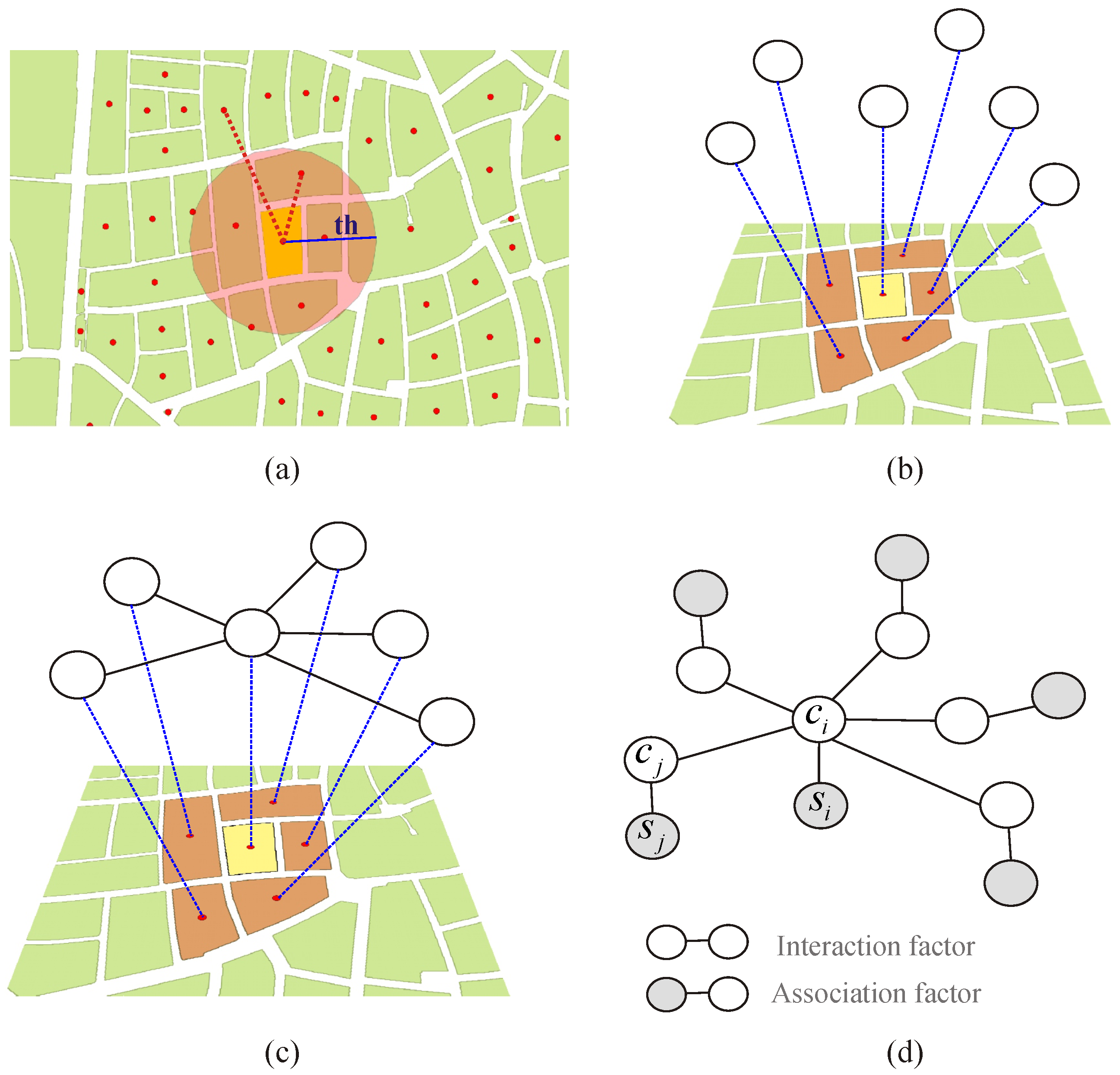
2.1. Context-Based Classification with Probabilistic Graphical Models

Probabilistic Graphical Models (PGMs) are used for modeling systems with many variables about which we want to reason. As it is frequently difficult to establish deterministic relations between variables, considering uncertainty is essential in many applications. In PGMs, uncertainty is modeled using probability theory. Probabilistic dependencies and conditional independencies between variables can be assumed or learned from data, and thus, the factorization of a joint probability distribution with many variables can be defined. The factorization enables reasoning on the system, since considerably fewer parameters are needed to represent a large distribution in its factorized form than as a joint distribution [35]. In the context of image classification, undirected PGMs are frequently used to encode the factorization of a conditional distribution P(C|S) , where C represents the image’s classification and S the observed image data. A simple factorization of such a distribution can be formulated as:
P ( C | S ) = 1 Z ( S ) e x p ( i I log p ( c i | s i ) + i I j N i ϕ i j ( c i , c j ) ) ,
where i is an image site, for example, a pixel, an image segment or, as in our case, an urban block, ci is the unknown class label of block i and si is a vector of attributes extracted from block i. The letter j denotes a block belonging to the set of neighbors Ni from block i. Z(S) is the partition function of the distribution, which scales the probabilities to the interval [0,1]. The so-called association factors log p ( c i | s i ) represent the likelihood terms or the prior probabilities of the classes for each block i, whereas the interaction factors ϕ i j ( c i , c j ) map each possible joint class assignment of ci and cj to a real positive number. Since the goal is to maximize Equation (1), in other words, to find the joint class assignment for all ci for which the conditional probability P(C|S) is maximum (this is commonly referred to as the estimation of the maximum a posteriori probability, or MAP solution), we may disregard the partition function Z(S) and reformulate Equation (1) as the following energy function:
E ( C , S ) = i I log p ( c i | s i ) + λ i I j N i ϕ i j ( c i , c j ) .
Since E ( C , S ) log ( P ( C | S ) ) , the classification C that maximizes Equation (1) can be inferred by minimizing Equation (2) [35]. This minimization is however NP-hard and must be performed computationally with an approximate inference algorithm. In this work, we used the max-sum loopy belief propagation algorithm [36], which is available in the PGM library OpenGM [37]. The comparable and at times superior performance of max-sum loopy belief propagation with respect to other algorithms has been demonstrated empirically in numerous applications requiring the estimation of the maximum a posteriori, also known as MAP, assignment [38].
As the number of neighboring relationships between blocks (expressed by the interaction factors) is significantly higher than the number of blocks (each of which is represented with one association factor), the weighting term λ was inserted in order to balance the influence of each type of factor in the energy function.

2.2. Model Parameterization and Neighborhood Definition Criteria

In this section, the models with which we performed context-based USTs classification are presented. The models vary regarding (i) the variables that comprise the interaction factors, (ii) the parameterization function of these factors and (iii) the criterion considered for defining pairwise neighborhood relationships between urban blocks. All models have in common the fact that a random forest classification model is used to compute the prior probabilities p ( c i | s i ) in the association factors. The Random Forest classifier consists of a large number of decision trees [39], each of which is fitted with randomly selected subsets of variables and samples. Each decision tree casts a vote on to which class each instance belongs. The proportion between the number of votes to each class and the total number of trees from the forest was regarded as the prior probability of that class given the observed block attributes. Because each tree is fitted with a different subset of samples and block attributes, the Random Forest algorithm has the advantage that it is robust against noise and over-fitting, even when the number of variables is high in relation to the number of samples. These advantages have led to the superior performance of Random Forest when compared to other powerful methods for classifying remote sensing images [40,41]. Furthermore, it can estimate the relevance of the variables during the fitting of the model. This feature of Random Forest can be applied both for dimensionality reduction, as well as for finding out which variables most influence the classification’s accuracy. For more details on the Random Forest algorithm, the reader is referred to the work of [42].
The most basic model with which we performed context-based UST classification is the standard Markov random field (MRF) model already presented in Equation (2). The interaction factors of this MRF model are parameterized by a simple Potts function as follows:
ϕ i j ( c i , c j ) = 0 if c i = c j 1 if c i c j .
Therefore, the interaction factors from this model penalize the energy function (Equation (2)) to the extent of one in cases where two neighboring blocks are assigned to two different UST classes. In practice, they produce a smoothing effect in the classification that does not consider the differences in the built-up structure and geometric shape of the two neighboring blocks.
The other three models with which we experimented fall under the category of so-called conditional random field (CRF) models. They differ from the MRF model regarding the variables comprising the interaction factors, as well as their parameterization functions. The names given to these models and their respective interaction factor functions are the following:
C R F 1 : ϕ ( s i , s j , c i , c j ) = 0 if c i = c j log s i s j 2 if c i c j .
C R F 2 : ϕ ( s i , s j , c i , c j ) = 0 if c i = c j log s i w s j w 1 if c i c j .
C R F 3 : ϕ ( S 2 i , j , c i , c j ) = 0 if c i = c j log S 2 i , j if c i c j .
When two neighboring blocks i and j are assigned to different classes, the model CRF 1 penalizes the energy function to the extent of the difference in the vectors of attributes from these blocks. This difference was computed using the Euclidean norm, also known as the L 2 -norm. Model CRF 2 differs from CRF 1 in that it penalizes the energy function when two neighboring blocks are assigned to different classes to the extent of the weighted difference between their vectors of attributes. The weight of each attribute was considered to be its normalized relevance estimated by the Random Forest algorithm. Variable importance estimation with Random Forest was performed with the mean accuracy decrease strategy [43]. For the computation of the difference between the vectors of attributes from blocks i and j, the values of each attribute from all blocks were firstly normalized so that the vectors’ difference is always in the interval [0,1], therefore the same scale of the association factors. The penalty in case of model CRF 3 is anti-proportional to the shape similarity S 2 i , j between the neighboring blocks i and j. Therefore, the more similar their geometric shapes, the higher the penalty gets if they are assigned to different classes. The shape similarity metric considered is the one proposed by [44].
Regarding the criterion for defining pairwise neighboring relationships between urban blocks, four criteria were explored. These are the following:
j N i if Fixed radius : d ( i , j ) < 240 m Adaptive radius : d ( i , j ) < l e n g t h i 1 , 5 d i s t . ( i , j ) < 300 m Nearest - neighbors ( NN ) : j 3 - NN ( i ) d ( i , j ) < 300 Region adjacency : if blocks i and j are adjacent ,
In the first three criteria above, d(i,j) denotes the Euclidean distance between the centers of mass from blocks i and j. The first criterion considers two blocks as neighbors when their centers of mass are not further than 240 m apart. This value was chosen because it is the rounded 80th percentile of the length from all blocks in the study area. The second criterion sets this distance threshold adaptively by multiplying the length of block i by 1.5 and establishing an upper limit of 300 m in order to avoid that large blocks contain an excessive number of neighbors. The third criterion defines neighboring relationships between each block i and its three nearest-neighbors. The upper distance limit of 300 m is also set to this criterion. This value was set as the upper limit because it is the upwardly rounded number of the maximum length of the blocks. The fourth criterion establishes neighboring relationships between two blocks if they can be considered adjacent to each other. The adjacencies between blocks were extracted according to the strategy described in [45].
Figure 1 depicts how association and interaction factors from the MRF model are created. The neighbors of each block are detected based on one of the criteria from Equation (7). In the case of Figure 1a, as an example, the first criterion from Equation (7) is applied. Each block’s unobserved class label is represented by a node (Figure 1b). Pairs of neighboring blocks are represented by an interaction factor containing the two unobserved labels (Figure 1c). Each block is also represented by an association factor containing the observed attributes of the block and its unobserved class label (Figure 1d).

2.3. Urban Blocks’ Attributes

The association factors represent the prior probabilities of each UST class given the blocks’ attributes. These probabilities are computed by a Random Forest classification model. The blocks attributes considered in this process are of three types, namely (i) attributes computed from extracted dark and bright areas (see the next paragraph), (ii) composition and disposition attributes computed from meaningful lines and polygons extracted inside each urban block and (iii) texture attributes computed from a digital elevation model (DEM) derived using the technique of interferometry [46].
Dark and bright areas were extracted from each block by applying threshold operations on the intensity and coherence images. Coherence is the complex cross-correlation coefficient from two co-registered SAR acquisitions obtained at the same satellite’s orbit. It can be computed for the whole scene by running a moving window over the image pair and estimating the coherence for each pixel. On coherence images, dark areas are mostly correlated with vegetation, shadow and water bodies, whereas bright areas frequently correspond to man-made structures whose geometries reflect a significant extent of the emitted SAR signal back to the sensor [46]. The pixel values of SAR intensity images represent the proportion of emitted signal that is backscattered from the respective area on the ground. On SAR intensity images, bright areas frequently appear due to the inherent effects of corner reflection and layover, whereas dark areas are frequently caused by the shadowing effect [46]. The shape, size and orientation of bright and dark areas in SAR intensity images from urban areas strongly correspond to the buildings shape and orientation [47,48]. Therefore, as valuable indicators of the built-up structure from each urban block, bright and dark areas were extracted from the SAR intensity image of each block. Bright areas were also extracted from the coherence images of each block. The 20th percentile of the SAR intensity images were selected as the threshold values under which pixels were considered dark, whereas pixels with values above the 80th percentile of the SAR intensity and coherence images were considered bright. Following this, connected components from bright and dark areas were produced using the 8-pixel connectivity criterion. Areas with a size smaller than 40 m2 were discarded from further analysis. This threshold value was chosen given the fact that the footprint of a house or building is hardly smaller than that. The remaining dark and bright areas had their size, compactness, perimeter-area ratio and length-to-width ratio computed. Table 1 shows which descriptive attributes were computed from the dark and bright areas and then submitted for the classification with the Random Forest algorithm. The parameters of some of these attributes were set empirically based on the image resolution and the typical area range and shape of different types of buildings in the test-site, namely single-family houses, apartment buildings and warehouses. When transferring the model to other cities, adjustments in the parameter values may be necessary. Alternatively, additional attributes with different parameter values may be submitted to the Random Forest algorithm, which is able to perform attribute relevance analysis and is robust to correlated variables [42].
The second type of attributes considered in the classification with the Random Forest algorithm refers to the composition and disposition attributes computed from meaningful polygon and line features extracted inside each urban block. As mentioned, the composition attributes describe the number, area proportion and general geometric properties of the features from each block, whereas the disposition attributes describe their relative spatial disposition inside the blocks. The procedures employed for extracting meaningful lines and polygons are described in detail in [49]. Figure 2 depicts the outcome of the main steps involved. The input of the line and polygon extraction procedures is the intensity image of each block, which is initially kept in acquisition coordinates (Figure 2a). The extracted lines and polygons, as well as the block boundaries are projected to the local coordinate system, i.e., Gauss–Kruger Zone 12 (Figure 2d,e). Finally, a network is created whose nodes are set at the center of mass of the extracted polygons. Edges of this network are established between polygons that are considered neighbors according to the criterion of 2-nearest-neighbors (Figure 2f). Table 2 and Table 3 show respectively the block attributes computed from the extracted lines and polygons. In Table 3, the attributes ‘Number of pairs of polygons parallel to each other’ and ‘Number of pairs of polygons parallel to each other’ refer to polygons whose center axes have relative orientation differences in the intervals 0 –15 and 75 –90 , respectively. The ‘Maximum pertinence’ attribute (also in Table 3) regards the adherence of the polygon to the size, compactness and length-to-width ratio of an ideal building polygon. This pertinence is in the range from 0–1, and it is computed in the polygon extraction strategy described in detail in [49]. The attributes computed from the networks created from the extracted polygons are shown in Table 4.
As texture attributes, histograms of oriented gradients (HOGs) [50] were extracted from the DEM of each block. A single un-normalized histogram with eight bins was accumulated for each block. The values of the eight bins were considered then as block attributes.

3. Experiments

3.1. Image and Auxiliary Data

The image data used in all experiments are a set of single look complex images acquired by the TerraSAR-X satellite operating in High-Resolution Spotlight mode [53]. The images were kindly provided by the German Aerospace Center (DLR) after the submission and acceptance of a research proposal. They have a nominal spatial resolution of approximately 1.1 m, which is the lowest accepted resolution for distinguishing buildings in urban environments [47,54,55]. The image set is comprised of four images acquired as two interferometric pairs, of which one pair was acquired at the satellite’s ascending orbit and the other at descending orbit. The use of images from both orbits has significantly increased the potential for extracting meaningful attributes from the blocks, as discussed in [49]. The minimum and maximum incidence angles of all four acquisitions range from 22 –26 , which has avoided that either the layover or shadowing effects become critical [48]. The only auxiliary data used in this work are the network of streets, rivers and railroads, as well as the official UST map from the city of Munich (Germany). Both of these datasets were kindly provided in shapefile (.shp) format by the city hall’s Department of Health and Environment (Referat fuer Gesundheit und Umwelt). The network of streets, rivers and railroads was used for extracting the urban blocks from the study site. This task was accomplished by simply extracting the closed areas limited by the streets, rivers and railroads. The official UST map was considered as ground truth data and used for collecting training samples and assessing the classifications’ global and per-class accuracies.

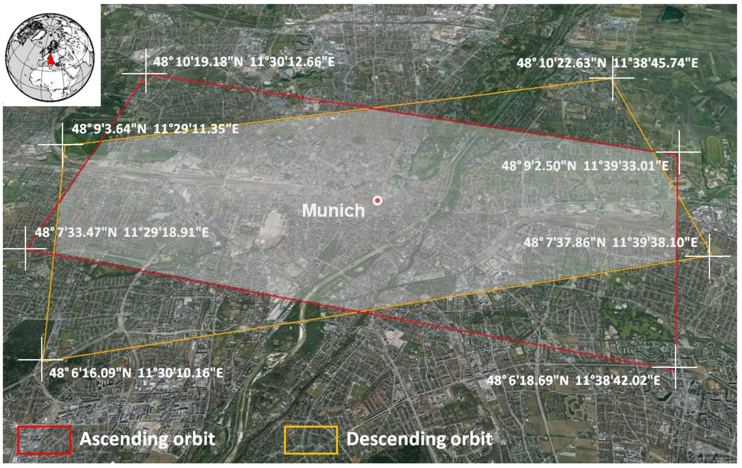
3.2. Study Area and Urban Structure Type Classes

The four TerraSAR-X acquisitions cover most of the central area of Munich (Germany). Figure 3 shows the exact footprints of the master images from the two interferometric pairs utilized in this work. Each footprint covers an area of approximately 10 × 5 km. The study area was defined as the intersection of these two footprints, which is highlighted in Figure 3. Its central point is located in the historical center of the city. In total, the study area is comprised of 1,695 urban blocks originally assigned to 27 UST classes. However, because many of these classes have a low number of instances in the study area, a semantic generalization of the original classes was undertaken. This procedure grouped the initial 27 UST classes based on their structural and functional similarities into five general ones, namely, dense block development (DBD), detached and semi-detached housing (DSDH), large buildings and industrial areas (LBIA), regular block development (RBD) and parks, squares and vegetated areas (PSVA). A spatial generalization was also undertaken at blocks originally assigned to more than one UST class. These mixed blocks, corresponding to approximately 21% of the blocks from the study area, were assigned to the UST class with the largest area inside them. The outcome of the class and spatial generalization process is a UST ground-truth map with five structurally- and semantically-coherent classes and in which each block is assigned to a single UST class. As mentioned, this map was used for the training of the models and the evaluation of the classifications.
Munich was chosen as our study area due to the following advantages: (i) ample availability of TerraSAR-X acquisitions from this city, (ii) the existence of reliable auxiliary and ground-truth data and (iii) the fact that its morphology is similar to other medium to large European cities.

3.3. Classification Experiments

All context-based classification models we presented in Section 2.2 contain association factors that compute the prior probabilities of the classes given the attributes of each block. This computation is performed with the Random Forest algorithm. By assigning to each block the class with the highest prior probability, a standard (as opposed to context-based) classification is produced. This standard classification was performed by firstly selecting the training samples from each class out of the 1695 blocks of the study area. The number of samples collected for each class was 63, which is half the number of instances from the UST class with the least number of instances in the study area, namely large buildings and industrial areas. This added to a total of 315 training samples (5 × 63). The remaining 1,380 blocks were considered in the evaluation of the classifications. The Random Forest algorithm was set to contain one-thousand trees, each of which was firstly fitted with a random set of samples and a random set of the block attributes presented in Section 2.3. In this step, the relevance of all block attributes was computed, and the attributes with relevance below average were discarded. Following the, the Random Forest classifier was fitted once again, but now considering only the attributes that were not discarded in the first step. The new relevance values, i.e., from the second Random Forest model fitting, were considered in the parameterization of the interaction factors from model CRF 3, as explained in Section 2.2. As mentioned, the relevance of the attributes was computed using the mean accuracy decrease strategy presented in [43].
The initial set of attributes, i.e., before the first fitting of the Random Forest model and the discarding of irrelevant attributes, contained 372 attributes. These comprise (i) the attributes from Table 1 computed from the master SAR intensity images from both orbits (36 × 2), (ii) the bright areas’ attributes from Table 1 computed from the coherence images from both orbits (18 × 2), (iii) the line attributes from Table 2 computed from the master SAR intensity images from both orbits (29 × 2), (iv) the polygon attributes from Table 3 computed from the master SAR intensity images from both orbits (44 × 2), (v) the network attributes from Table 4 computed from the polygons extracted out of the master SAR intensity images from both orbits (55 × 2) and (vi) the HOG attributes extracted from the DEM derived from the interferometric pair of SAR intensity images from the ascending orbit (8). After the elimination of irrelevant ones, 96 attributes were left for the second and final fitting of the Random Forest classification model.

4. Results

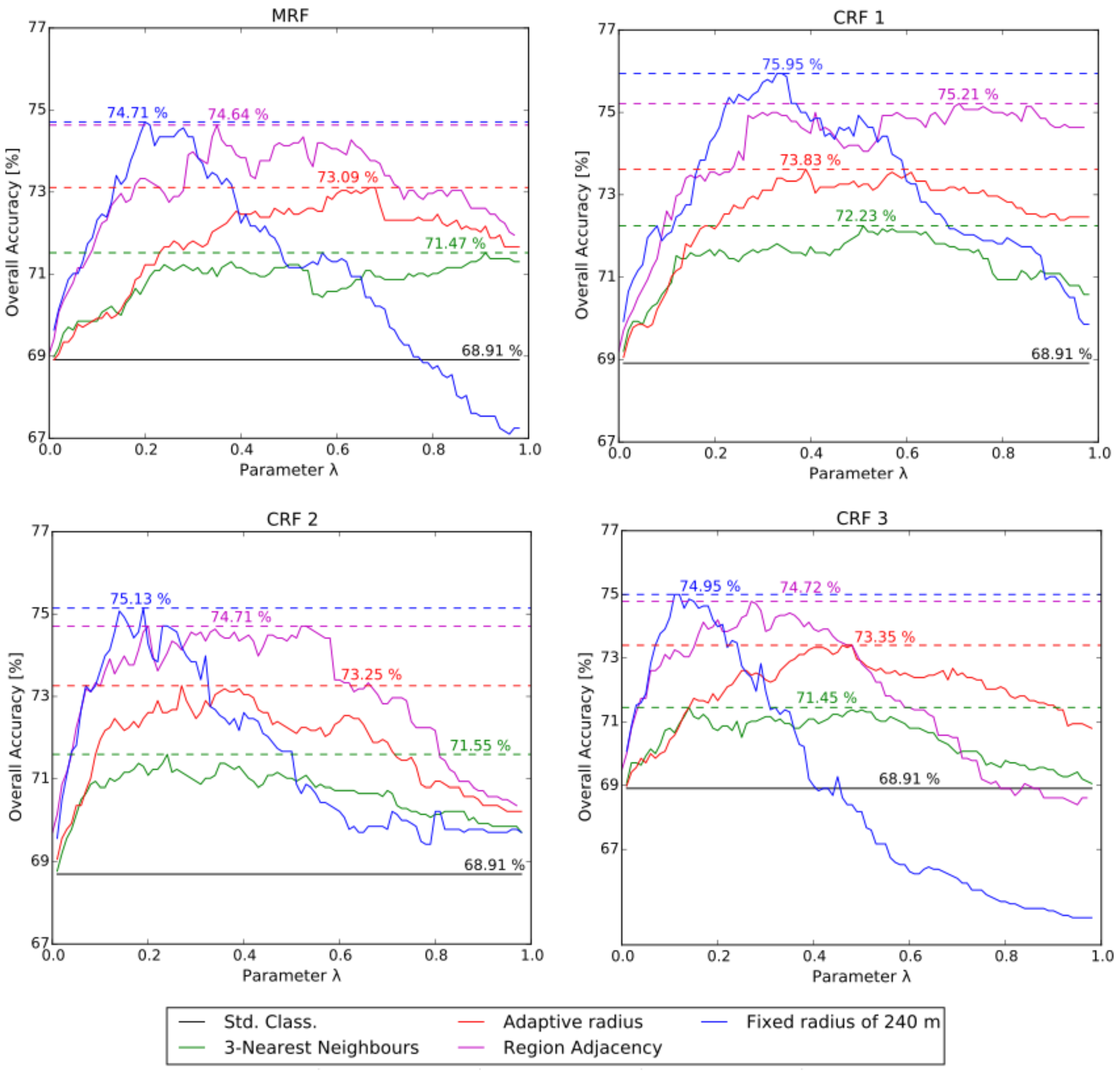
4.1. Model Comparison

Each of the four models was tested in combination with the four neighborhood definition criteria presented in Equation (7). Each of these combinations was evaluated with the λ parameter varying in steps of 0.01 from 0.01 up to 1.0, and the obtained overall accuracies were recorded. As mentioned, λ is a weighting term that balances the influence of each type of factor in the energy function. Figure 4 shows for each model a plot-graph of the overall accuracy obtained with each λ value. The colors of the lines indicate the neighborhood definition criterion. The horizontal black lines in each of the plot-graphs indicate the overall accuracy obtained when applying the Random Forest algorithm with the descriptive attributes presented in Section 2.3. The accuracy obtained with this classification model is 68.91%. It can be observed that, with all four models, the highest accuracy values were obtained when the neighborhood of each block was defined by the criterion of a fixed radius of 240 m, followed by the criterion of region adjacency. The overall highest accuracies, when considering each neighborhood definition criterion separately, were obtained with model CRF 1, followed by models CRF 2 and CRF 3. Thus, when combining model CRF 1 with the neighborhood defined by the criterion of a fixed radius of 240 m, the highest improvement in the overall accuracy in relation to the standard classification was obtained, namely 7.05%.

4.2. Accuracy Analysis

In this section, we analyze in more detail the quality of the standard classification and the context-based classification obtained with model CRF 1 and the neighborhood definition criterion of a fixed radius of 240 m. The reason for us focusing on this specific context-based classification model is that it was the one that achieved the highest accuracy improvement in relation to the standard classification, as can be seen in Figure 4. Figure 5 depicts these two classifications, as well as the ground-truth map of the study-site. It can be observed that the spatial distribution of the UST classes in the ground-truth map is not random. The extent to which instances of the same class are grouped into clusters can be analyzed with the assortativity measure proposed by [56]. To the best of our knowledge, this is the only measure available for global spatial autocorrelation of categorical data. Given a criterion for establishing pairwise neighboring relationships between blocks, this measure is 1.0 when every pair of neighboring blocks is assigned to the same class. The assortativity measure is −1.0 when these blocks are assigned always to two different classes. Considering the neighborhood criterion of a fixed radius of 240 m, the ground-truth map in Figure 5c has an assortativity of 0.45. This is evidence that the classification accuracy can be improved if the context of each block is considered in its class assignment.
Indeed, a visual analysis of the standard (Figure 5a) and context-based (Figure 5b) classifications shows that the latter is more similar to the ground-truth map than the former. In order to verify this quantitatively, we resorted to commonly-used accuracy analysis measures derived from the confusion matrix of a classification, namely the global Kappa index, as well as the per-class user’s and producer’s accuracy indexes [57]. Table 5 shows the confusion matrices of the standard, as well as the context-based classification. The overall accuracy of the standard classification is 68.91%, and its Kappa index is 0.57. The context-based classification in its turn achieved an overall accuracy of 75.95% and a Kappa index of 0.65. It can be observed from the confusion matrices that almost all the producer’s and user’s accuracies of all classes increased when context was considered in the classification. The only exception is the user’s accuracy of class ‘parks and vegetated areas’, which slightly decreased in the context-based classification. This might be due to over-smoothing, given that instances of this class frequently appear surrounded by residential and even commercial blocks. Indeed, most false-negative errors of this class that appeared in the context-based classification and were originally not to be seen at the standard one were assigned to class ‘dense block development’. Furthermore, the number of false-negative errors from class ‘detached and semi-detached housing’ assigned to class ‘regular block development’ slightly increased in the context-based classification. Other than that, all numbers outside the diagonal of the confusion matrix have decreased when context was considered in the classification.

5. Discussion

The classification of USTs based on remote sensing imagery is a challenging task. There are two main reasons for this. The first is that some classes are defined by functional and cultural aspects more than others. These classes can be successfully classified only to the extent that they also have typical structural characteristics. For example, it is impossible to directly ascertain based on objective image attributes whether a block is of residential or commercial use. Luckily, residential areas are frequently associated with a certain type of built-up structure, usually characterized by the presence of vegetation and of small to medium-sized constructions. However, it is difficult to establish a consistent correlation between socio-economic and functional aspects, which are subjective, and structural aspects, which are objective. The second reason is that urban blocks from the same class may be very heterogeneous regarding their shape, orientation and the geometric structure and spatial disposition of the urban features inside them. In fact, no pair of blocks from the same class is ever identical. Furthermore, characteristics that are typical of a class may be found in instances from other classes, as well. This means it is challenging to identify expressive image-derived attributes for block-based UST classification. Resorting to a powerful classifier and to a larger number of training samples is an advisable measure. However, selecting a large number of training samples may not be possible for some classes. In these cases, it is necessary to consider a smaller number of more general classes, each of which is the result of a merging of classes with similar structural characteristics. Despite these limitations, the automatic classification of USTs based on remote sensing images provides a subjectivity-free and consistent categorization of urban blocks according to their structural characteristics. Such objective grouping of blocks according to their built-up structure is relevant for several urban studies, as well as for urban planning in general.
Independently of the methods applied, block-based classification of USTs requires images with adequate spatial resolution so that urban blocks can be effectively characterized regarding their UST. Although the medium resolution of TerraSAR-X StripMap (≈3 m) and Sentinel-1 (≈5 m) images is most likely insufficient for that task, the TerraSAR-X and COSMO-SkyMed satellites operating in spotlight mode provide images with appropriate spatial resolution (≈1 m) for distinguishing USTs at the block level. This is relevant regarding the mapping and monitoring of USTs in parts of the world where airborne imagery may still be lacking or hard to obtain. The transferability of ours and any other UST classification models is however limited by the environmental, cultural and, more generally, geographic peculiarities of different cities. These peculiarities lead to the necessity of adjusting the model’s parameters and eventually considering other attributes in the classification.
In this paper, we proposed an approach for classifying USTs using TerraSAR-X Spotlight imagery acquired at the satellite’s ascending and descending orbits. Instead of considering attributes computed from a previously performed land cover classification, as most of the related work has done, our approach is based on attributes that describe the geometric characteristics and spatial disposition of lines and polygons extracted inside each block. Our main contribution is however to demonstrate that considering the context of each block in the classification is expected to improve the classification accuracy, assuming though that the spatial distribution of the classes is not random. This assumption holds well for large cities of the Western world that frequently have urban zoning laws. It should be noticed that in cities where such laws are lacking or are not being respected, the advantage of considering the context of the urban blocks in their classification might be significantly limited. It is safe to say though that PGMs are the most sound and flexible statistical approach for modeling contextual influences between geographical entities. The reason for this is that the constituent parts of a PGM, namely its structure, association and interaction factors and inference algorithm, are independent of each other, which enables easy adaption to other study sites, input image data and attribute sets without any effect on the statistical formalities of probability laws. This leads to the fact that different block attributes extracted from different images could be used for computing the prior class probabilities of the blocks. The only parameter that must be tuned in all cases is the lambda parameter, which compensates for the different number of association and interaction factors.
We conclude this paper by stressing the necessity of further work on how to tackle the problem of mixed blocks, i.e., blocks officially assigned to more than one class. As mentioned above, a significant percentage of blocks from our study area is officially assigned to more than one class. Novack and Stilla [58] proposed a strategy for detecting mixed blocks based on the classification instability of the blocks. However, the problem seems to lie more on how to segment mixed blocks according to the different USTs inside it. To the best of our knowledge, an efficient solution to this issue is still to appear in the specialized literature.

Author Contributions

T.N. performed all the data processing as well as the analysis of the results. U.S. supervised this research and contributed to the writing of the manuscript.

Funding

This research was funded by the Deutscher Akademischer Austauschdienst (DAAD) under grant number A/10/71506.

Acknowledgments

We acknowledge the Deutsche Forschungsgemeinschaft (DFG) within the funding program Open Access Publishing, by the Baden-Württemberg Ministry of Science, Research and the Arts and by Ruprecht-Karls-Universität Heidelberg.

Conflicts of Interest

The authors declare no conflict of interest.

References

  1. United Nations. World Urbanization Prospects: The 2017 Revision; Technical Report; United Nations Department of Economic and Social Affairs, Population Division: New York, NY, USA, 2017. [Google Scholar]
  2. Bundesamt, U. Siedlungs-und Verkehrflaeche. 2015. Available online: https://www.umweltbundesamt.de/daten/flaeche-boden-land-oekosysteme/flaeche/siedlungs-verkehrsflaeche (accessed on 23 May 2018).
  3. Pauleit, S.; Duhme, F. Assessing the environmental performance of land cover types for urban planning. Landsc. Urban Plan. 2000, 52, 1–20. [Google Scholar] [CrossRef]
  4. Novack, T.; Stilla, U. Discriminative learning of conditional random fields applied to the classification of urban settlement types. Gemeinsame Tagung 2014 der DGfK, der DGPF, der GfGI und des GiN. 2014. Available online: https://www.pf.bgu.tum.de/pub/2014/novack_co_stilla_dgpf14_pap.pdf (accessed on 23 May 2017).
  5. Heinzel, J.; Kemper, T. Automated metric characterization of urban structure using building decomposition from very high resolution imagery. Int. J. Appl. Earth Obs. Geoinf. 2015, 35, 151–160. [Google Scholar] [CrossRef]
  6. Bach, P.; Staalesen, S.; McCarthy, D.; Deletic, A. Revisiting land use classification and spatial aggregation for modeling integrated urban water systems. Landsc. Urban Plan. 2015, 143, 43–55. [Google Scholar] [CrossRef]
  7. Baud, I.; Kuffer, M.; Pfeffer, K.; Sliuzas, R.; Karuppannan, S. Understanding heterogeneity in metropolitan India: The added value of remote sensing data for analyzing sub-standard residential areas. Int. J. Appl. Earth Obs. Geoinf. 2010, 12, 359–374. [Google Scholar] [CrossRef]
  8. Yu, B.; Liu, H.; Wu, J.; Hu, Y.; Zhang, L. Automated derivation of urban building density information using airborne LiDAR data and object-based method. Landsc. Urban Plan. 2010, 98, 210–219. [Google Scholar] [CrossRef]
  9. Banzhaf, E.; Hoefer, R. Monitoring urban structure types as spatial indicators with CIR aerial photographs for a more effective urban environmental management. IEEE J. Sel. Top. Appl. Earth Obs. Remote Sens. 2008, 1, 129–138. [Google Scholar] [CrossRef]
  10. Novack, T.; Kux, H. Urban land cover and land use classification of an informal settlement area using the open-source knowledge-based system InterIMAGE. J. Spat. Sci. 2010, 55, 23–41. [Google Scholar] [CrossRef]
  11. Heiden, U.; Heldens, W.; Roessner, S.; Segl, K.; Esch, T.; Mueller, A. Urban structure type characterization using hyperspectral remote sensing and height information. Landsc. Urban Plan. 2012, 105, 361–375. [Google Scholar] [CrossRef]
  12. Voltersen, M.; Berger, C.; Hese, S.; Schmullius, C. Object-based land cover mapping and comprehensive feature calculation for an automated derivation of urban structure types at block level. Remote Sens. Environ. 2014, 154, 192–201. [Google Scholar] [CrossRef]
  13. Novack, T.; Kux, H.; Feitosa, R.; Costa, G. A knowledge-based, transferable approach for block based urban land use classification. Int. J. Remote Sens. 2014, 35, 4739–4757. [Google Scholar] [CrossRef]
  14. Walde, I.; Hese, S.; Berger, C.; Schmullius, C. From land cover-graphs to urban structure types. Int. J. Geogr. Inf. Sci. 2014, 28, 584–609. [Google Scholar] [CrossRef]
  15. Walde, I.; Hese, S.; Berger, C.; Schmullius, C. Graph-based mapping of urban structure types from high-resolution satellite image objects-case study of the german cities Rostock and Erfurt. IEEE Geosci. Remote Sens. Lett. 2013, 10, 932–936. [Google Scholar] [CrossRef]
  16. Wurm, M.; Taubenboeck, H.; Dech, S. Urban structuring using multi-sensoral remote sensing data by the examples of german cities Cologne and Dresden. In Proceedings of the 2009 Joint Urban Remote Sensing Event, Shanghai, China, 20–22 May 2009; pp. 1–8. [Google Scholar]
  17. Schmidt, M.; Esch, T.; Klein, D.; Thiel, M.; Dech, S. Estimation of building density using TerraSAR X-data. In Proceedings of the IEEE International Geoscience and Remote Sensing Symposium, Honolulu, HI, USA, 25–30 July 2010; pp. 1936–1939. [Google Scholar]
  18. Duque, J.C.; Patino, J.E.; Ruiz, L.A.; Pardo-Pascual, J.E. Measuring intra-urban poverty using land cover and texture metrics derived from remote sensing data. Landsc. Urban Plan. 2015, 135, 11–21. [Google Scholar] [CrossRef]
  19. Wurm, M.; Taubenboeck, H.; Dech, S. Quantification of Urban Structure on Building Block Level Utilizing Multisensoral Remote Sensing Data. In Proceedings of the SPIE 7831 Earth Resources and Environmental Remote Sensing/GIS Applications, Toulouse, France, 21–23 September 2010. [Google Scholar]
  20. Huck, A.; Hese, S.; Banzhaf, E. Delineating parameters for object-based urban structure mapping in Santiago de Chile using QuickBird data. ISPRS Hannover 2011 Worshop. 2011. Available online: https://pdfs.semanticscholar.org/043d/738e95d2e6ce6d849c53872446da3ad31d3f.pdf?_ga=2.222760539.1140457605.1527174813-91830153.1527174813 (accessed on 23 May 2017).
  21. Coseo, P.; Larsen, L. How factors of land use/land cover, building configuration, and adjacent heat sources and sinks explain urban heat islands in Chicago. Landsc. Urban Plan. 2014, 125, 117–129. [Google Scholar] [CrossRef]
  22. Lackner, M.; Conway, T. Determining land use information from land cover through an object oriented classification of IKONOS imagery. Can. J. Remote Sens. 2008, 34, 77–92. [Google Scholar] [CrossRef]
  23. Linden, S.; Hostert, P. The influence of urban structures on impervious surface maps from airborne hyperspectral data. Remote Sens. Environ. 2009, 113, 2298–2305. [Google Scholar] [CrossRef]
  24. Benz, U.; Hofmann, P.; Willhauck, G.; Lingenfelder, I.; Heynen, M. Multi resolution object oriented fuzzy analysis of remote sensing data for GIS ready information. ISPRS J. Photogramm. Remote Sens. 2004, 58, 239–258. [Google Scholar] [CrossRef]
  25. Blaschke, T. Object based image analysis for remote sensing. ISPRS J. Photogramm. Remote Sens. 2010, 65, 2–16. [Google Scholar] [CrossRef]
  26. Berlin. Bericht zur Dokumentation der Kartiereinheiten und der Aktualisierung des Datenbestandes. 2010. Available online: http://www.stadtentwicklung.berlin.de/umwelt/umweltatlas/dd607_04.htmlk15 (accessed on 24 May 2017).
  27. Hecht, R.; Herold, H.; Meinel, G.; Buchroithner, M. Automatic Derivation of Urban Structure Types from Topographic Maps by Means of Image Analysis and Machine Learning. In Proceedings of the 26th International Cartographic Conference, Dresden, Germany, 25–30 August 2013. [Google Scholar]
  28. Vanderhaegen, S.; Canters, F. Developing urban metrics to describe the morphology or urban areas at block level. Int. Arch. Photogramm. Remote Sens. Spat. Inf. Sci. 2010, 38, 192–197. [Google Scholar]
  29. Hermosillaa, T.; Ruiza, L.; Recioa, J.; Cambra-Lopezb, M. Assessing contextual descriptive features for plot-based classification of urban areas. Landsc. Urban Plan. 2012, 106, 124–137. [Google Scholar] [CrossRef]
  30. Tobler, W. A computer movie simulating urban growth in the Detroit region. Econ. Geogr. 1970, 46, 234–240. [Google Scholar] [CrossRef]
  31. Dekker, R.J. Texture analysis and classification of ERS SAR images for map updating of urban areas in the Netherlands. IEEE Trans. Geosci. Remote Sens. 2003, 41, 1950–1958. [Google Scholar] [CrossRef]
  32. Gamba, P.; Aldrighi, M. SAR data classification of urban areas by means of segmentation techniques and ancillary optical data. IEEE J. Sel. Top. Appl. Earth Obs. Remote Sens. 2012, 5, 1140–1148. [Google Scholar] [CrossRef]
  33. Salentinig, A.; Gamba, P. A general framework for urban area extraction exploiting multiresolution SAR data fusion. IEEE J. Sel. Top. Appl. Earth Obs. Remote Sens. 2016, 9, 2009–2018. [Google Scholar] [CrossRef]
  34. Amitrano, D.; Belfiore, V.; Cecinati, F.; Martino, D.; Iodice, A.; Mathieu, P.-P.; Medagli, S.; Poreh, D.; Riccio, D.; Ruello, G. Urban areas enhancement in multitemporal SAR RGB images using adaptive coherence window and texture information. IEEE J. Sel. Top. Appl. Earth Obs. Remote Sens. 2016, 9, 3740–3752. [Google Scholar] [CrossRef]
  35. Koller, D.; Friedman, N. Probabilistic Graphical Models: Principles and Techniques; MIT Press: London, UK, 2009. [Google Scholar]
  36. Kschischang, F.; Frey, B.; Loelinger, H. Factor graphs and the sum-product algorithm. IEEE Trans. Inf. Theory 2001, 47, 498–519. [Google Scholar] [CrossRef]
  37. Andres, B.; Kappes, J.H.; Koethe, U.; Schnoerr, C.; Hamprecht, F.A. An empirical comparison of inference algorithms for graphical models with higher order factors using OpenGM. In Pattern Recognition; Lecture Notes in Computer Science; Goesele, M., Roth, S., Kuijper, A., Schiele, B., Schindler, K., Eds.; Springer: Berlin/Heidelberg, Germany, 2010; Volume 6376, pp. 353–362. [Google Scholar]
  38. Szeliski, R.; Scharstein, D.; Veksler, O.; Kolmogorov, V.; Agarwala, A.; Tappen, M.; Rother, C. A comparative study of energy minimization methods for Markov Random Fields with smoothness-based priors. IEEE Trans. Pattern Anal. Mach. Intell. 2008, 30, 1068–1080. [Google Scholar] [CrossRef] [PubMed]
  39. Quinlan, J.R. Simplifying decision trees. Int. J. Man Mach. Stud. 1987, 27, 221–234. [Google Scholar] [CrossRef]
  40. Hariharan, S.; Tirodkar, S.; Bhattacharya, A. Polarimetric SAR decomposition parameter subset selection and their optimal dynamic range evaluation for urban area classification using random forest. Int. J. Appl. Earth Obs. Geoinf. 2016, 44, 144–158. [Google Scholar] [CrossRef]
  41. Du, P.; Samat, A.; Waske, B.; Liu, S.; Li, Z. Random forest and Rotation Forest for fully polarized SAR image classification using polarimetric and spatial features. ISPRS J. Photogramm. Remote Sens. 2015, 105, 38–53. [Google Scholar] [CrossRef]
  42. Breiman, L. Random forests. Mach. Learn. 2001, 1, 5–32. [Google Scholar] [CrossRef]
  43. Hastie, T.; Tibshirani, R.; Friedman, J. The Elements of Statistical Learning; Springer: New York, NY, USA, 2001. [Google Scholar]
  44. Arkin, E.; Chew, L.; Huttenlocher, D.; Kedem, K.; Mitchell, J. An efficiently computable metric for comparing polygonal shapes. IEEE Trans. Pattern Anal. Mach. Intell. 1991, 13, 209–216. [Google Scholar] [CrossRef]
  45. Novack, N.; Stilla, U. Context-based classification of urban blocks according to their built-up structure. PFG J. Photogramm. Remote Sens. Geoinf. Sci. 2017, 85, 365–376. [Google Scholar] [CrossRef]
  46. Woodhouse, I. Introduction to Microwave Remote Sensing; CRC Press: Bocaton, FL, USA, 2006. [Google Scholar]
  47. Stilla, U. High resolution radar imaging of urban areas. In Photogrammetric Week 07; Fritsch, F., Ed.; Wichmann: Berlin/Heidelberg, Germany, 2007; pp. 149–158. [Google Scholar]
  48. Stilla, U.; Soergel, U.; Thoennessen, U. Potential and limits of InSAR data for building reconstruction in built up areas. ISPRS J. Photogramm. Remote Sens. 2003, 58, 113–123. [Google Scholar] [CrossRef]
  49. Novack, T. Context-based Classification of Urban Structure Types Using Spaceborne InSAR Images. Ph.D. Thesis, Technische Universität München, München, Germany, 2016; 121p. [Google Scholar]
  50. Dalal, N.; Triggs, B. Histograms of Oriented Gradients for Human Detection. In Proceedings of the IEEE Computer Society Conference on Computer Vision and Pattern Recognition, San Diego, CA, USA, 20–25 June 2005; pp. 886–893. [Google Scholar]
  51. West, D.B. Introduction to Graph Theory; Prentice Hall: Upper Saddle River, NJ, USA, 2001; p. 512. [Google Scholar]
  52. Moran, P. Notes on continuos stochastic phenomena. Biometrika 1950, 37, 17–23. [Google Scholar] [CrossRef] [PubMed]
  53. DLR—Deutsches Zentrum für Luft und Raumfahrt. The Title of the Cited Contribution. TerraSAR-X—The German Radar Eye in Space. 2009. Available online: http://www.dlr.de/eo/Portaldata/64/Resources/dokumente/TSX_brosch.pdf (accessed on 23 May 2018).
  54. Tison, C.; Tupin, F. Estimation of urban DSM from mono-aspect InSAR images. In Radar Remote Sensing of Urban Areas; Springer: Berlin/Heidelberg, Germany, 2010; pp. 161–185. [Google Scholar]
  55. Chen, Z.; Zhang, Y.; Guindon, B.; Esch, T.; Roth, A.; Shang, J. Urban land use mapping using high resolution SAR data based on density analysis and contextual information. Can. J. Remote Sens. 2012, 386, 738–749. [Google Scholar] [CrossRef]
  56. Newman, M. Mixing patterns in networks. Phys. Rev. 2003, 67, 1–14. [Google Scholar] [CrossRef] [PubMed]
  57. Congalton, R.G.; Green, K. Assessing the Accuracy of Remotely Sensed Data: Principles and Practices; Mapping Science Series; Lewis Publishers: New York, NY, USA, 1999. [Google Scholar]
  58. Novack, T.; Stilla, U. Classification of urban settlements types based on space-borne SAR datasets. ISPRS Ann. Photogramm. Remote Sens. Spat. Inf. Sci. 2014, 2, 55–66. [Google Scholar] [CrossRef]
Figure 1. Construction of a simple undirected probabilistic graphical model for the classification of urban structure types. (a) Blocks are considered neighbors if the Euclidean distance between their centers of mass is not larger than a threshold (th). (b) Each block’s unobserved class c i is represented in the graph by a node. (c) An edge is created between each pair of neighboring blocks, thus forming an interaction factor. (d) If it is defined that, besides its neighbors unobserved variable c j , c i also depends on its observed attributes s i . The number of association factors in the graph equals the number of blocks in the study site. The number of pairwise interaction factors in the graph equals the number of pairs of neighboring blocks.
Remotesensing 10 00842 g001
Figure 2. Outcome of the main steps involved in the computation of block attributes from extracted lines and polygons. (a) The input to the procedure is the intensity SAR image of each block. (b) Lines extracted from the input image. (c) Polygons extracted from the input image. (d) Lines and the block’s boundaries projected to the local coordinate system. (e) Polygons and the block’s boundaries projected to the local coordinate system. (f) Network created from the extracted polygons.
Remotesensing 10 00842 g002
Figure 3. The image data footprints and the study area. Each footprint covers an area of approximately 10 × 5 km. Their intersection area was defined as our study area. The central point coincides with the historical center of Munich (Germany).
Remotesensing 10 00842 g003
Figure 4. Plot-graphs of the overall accuracies obtained with the four different models explored in this work and with λ parameters varying from 0.01–1.0. The colors of the lines indicate the neighborhood definition criterion.
Remotesensing 10 00842 g004
Figure 5. Ground-truth map and the standard and context-based classifications. (a) Standard classification performed with the Random Forest algorithm, i.e., without considering context. (b) context-based classification performed with model CRF 1 and the neighborhood definition criterion of a fixed radius of 240 m. (c) The official urban structure type (UST) map of Munich generalized for five classes and considered as the ground-truth.
Remotesensing 10 00842 g005
Table 1. Urban blocks attributes computed from the extracted bright and dark areas. Bright and dark areas were extracted by applying threshold operations on the Synthetic Aperture Radar intensity and coherence images.
Dark and bright areas’ attributes:
    Number of bright areas
    Number of dark areas
    Number of bright areas larger than 200 pixels
    Number of dark areas larger than 200 pixels
    Number of bright areas larger than 500 pixels
    Number of dark areas larger than 500 pixels
    Number of bright areas larger than 1000 pixels
    Number of dark areas larger than 1000 pixels
    Sum of bright areas larger than 200 pixels/block’s area
    Sum of dark areas larger than 200 pixels/block’s area
    Sum of bright areas larger than 500 pixels/block’s area
    Sum of dark areas larger than 500 pixels/block’s area
    Sum of bright areas larger than 1000 pixels/block’s area
    Sum of dark areas larger than 1000 pixels/block’s area
    Sum of bright areas/block’s area
    Sum of dark areas/block’s area
    Total area of all bright areas
    Total area of all dark areas
    Mean area of all bright areas
    Mean area of all dark areas
    Maximum area among bright areas
    Maximum area among dark areas
    Standard deviation of the area of all bright areas
    Standard deviation of the area of all dark areas
    Maximum compactness among bright areas
    Maximum compactness among dark areas
    Compactness of the largest bright area
    Compactness of the largest dark area
    Maximum length-to-width ratio among bright areas
    Maximum length-to-width ratio among dark areas
    Minimum perimeter-area ratio among bright areas
    Minimum perimeter-area ratio among dark areas
    Number of bright areas with length-to-width ratio higher than 5
    Number of dark areas with length-to-width ratio higher than 5
    Number of bright areas with length-to-width ratio higher than 10
    Number of dark areas with length-to-width ratio higher than 10
Table 2. Attributes computed from the lines extracted from the Synthetic Aperture Radar intensity images of each block. The line extraction procedure is described in detail in [49].
Line attributes:
    Maximum line length
    Mean angle difference between a line and its closest line
    Mean angle diff. between a line and the block boundary closest to it
    Mean angle diff. between a line and the block boundary most parallel to it
    Mean angle diff. between a line and the line most parallel to it
    Mean angle diff. between a line and the line most perpendicular to it
    Mean distance between a line and its closest line
    Mean distance between a line and the line most parallel to it
    Mean distance between a line and the line most perpendicular to it
    Mean distance between a line and the block boundary closest to it
    Mean distance between a line and the block boundary most parallel to it
    Mean distance between a line and the block boundary most perpendicular to it
    Mean orientation of the lines
    Mean length of the lines
    Min. angle diff. between a line and the block boundary closest to it
    Min. distance between a line and the line most parallel to it
    Min. distance between a line and the line most perpendicular to it
    Min. distance between a line and the block boundary most parallel to it
    Min. distance between a line and the block boundary most perpendicular to it
    Number of lines
    Number of lines longer than 50 m
    Number of lines longer than 100 m
    Std. dev. of angle difference between a line and its closest line
    Std. dev. of distance between a line and its closest block boundary
    Std. dev. of distance between a line and its closest line
    Std. dev. of distance between a line and the line most parallel to it
    Std. dev. of distance between a line and the line most perpendicular to it
    Std. dev. of the lines length
    Std. dev. of the orientation of all lines
Table 3. Attributes computed from the polygons extracted from the SAR intensity image of each block. The polygon extraction procedure is described in detail in Novack [49]. * The pertinence of the polygon to an ideal building polygon shape. The computation of this pertinence is demonstrated in Novack and Stilla [45].
Polygon attributes:
    Maximum pertinence *
    Mean area
    Mean angle difference between a polygon and its closest block boundary
    Mean distance between a polygon and its closest block boundary
    Mean distance between a polygon and the polygon most parallel to it
    Mean distance between a polygon and the polygon most perpendicular to it
    Mean, max. and std. dev. of the polygons area
    Mean, max. and std. dev. of the polygons length-to-width
    Mean, max. and std. dev. of the polygons compactness
    Mean, max. and std. dev. of the polygons orientation
    Number of pairs of polygons parallel to each other
    Number of pairs of polygons perpendicular to each other
    Number of polygons
    Number of polygons with area > 3rd, 4th and 5th 5-quantiles of the area values
    Number of polygons with pertinence > [0.05, 0.1, 0.15, 0.2, 0.3, 0.4, 0.5]
    Number of pol. with pertinence > [3rd, 4th, 5th] of the 5-quantiles of the pertinence values
    Std. dev. of the angle diff. between a polygon and its closest block boundary
    Std. dev. of the distance between a polygon and its closest block boundary
    Std. dev. of the distance between a polygon and the polygon most parallel to it
    Std. dev. of the distance between a polygon and the polygon most perpendicular to it
    Std. dev. of the polygons orientation
    3rd, 4th and 5th 5-quantiles of the polygons area
    3rd, 4th and 5th 5-quantiles of the pertinence values
Table 4. Attributes computed from the network of polygons extracted inside each block.
Network structure attributes:
    Density of the graph [51]
    Highest mean membership of two connected nodes
    Mean node pertinence
    Membership value of the node with highest membership
    Number of nodes
    Number of edges
    Number of edges/number of nodes
    Number of edges connecting parallel nodes
    Number of edges connecting parallel nodes/number of edges
    Number of edges connecting parallel nodes/Number of edges connecting perpendicular nodes
    Number of edges connecting perpendicular nodes
    Number of edges connecting perpendicular nodes/number of edges
    Std. dev. of the membership from the two connected nodes with highest membership mean
Network Moran’sIof attributes [52]:
    Area
    Distance to closest block boundary
    Length to width ratio
    Orientation
    Orientation difference to closest block boundary
    Rectangular fit
    For each of the six attributes above, the following measures were computed:
       Expected I based on random permutation of the values
       Expected I under normality assumption
       Difference between I and expected I based on random permutations
       Difference between I and expected I under normality assumption
       p-value of I based on random permutation of the values
       p-value of I under the normality assumption (one-sided)
Table 5. The confusion matrices of the standard and best context-based classifications. The best contextual classification was obtained with model CRF 1 and the neighborhood definition criterion of a fixed radius of 240 m. The overall accuracies achieved by the standard and contextual classifications are 68.91% and 75.95%, respectively. The respective Kappa indices are 0.57 and 0.65. The considered classes are Parks and Vegetated Areas (PVA), Detached and Semi-Detached Housing (DSDH), Large Buildings and Industrial Areas (LBIA), Dense Block Development (DBD) and Regular Block Development (RBD).
PVADSDHLBIADBDRBDTotalUser’s Acc. (%)Prod.’s Acc. (%)
Std. class.:
PVA18410331521585.5884.40
DSDH221446123521965.7557.60
LBIA2542676267.7730.00
DBD325614914862878.1885.68
RBD76628649125635.5446.42
Total218250140573196
Ctxt. class.:
PVA17685121421581.8685.85
DSDH15155264121970.7765.12
LBIA4445456272.2541.66
DBD510335463462882.9488.63
RBD561234811925646.4855.86
Total205238108616213

