Natural Forest Mapping in the Andes (Peru): A Comparison of the Performance of Machine-Learning Algorithms

Abstract

The Andes mountain forests are sparse relict populations of tree species that grow in association with local native shrubland species. The identification of forest conditions for conservation in areas such as these is based on remote sensing techniques and classification methods. However, the classification of Andes mountain forests is difficult because of noise in the reflectance data within land cover classes. The noise is the result of variations in terrain illumination resulting from complex topography and the mixture of different land cover types occurring at the sub-pixel level. Considering these issues, the selection of an optimum classification method to obtain accurate results is very important to support conservation activities. We carried out comparative non-parametric statistical analyses on the performance of several classifiers produced by three supervised machine-learning algorithms: Random Forest (RF), Support Vector Machine (SVM), and k-Nearest Neighbor (kNN). The SVM and RF methods were not significantly different in their ability to separate Andes mountain forest and shrubland land cover classes, and their best classifiers showed a significantly better classification accuracy (AUC values 0.81 and 0.79 respectively) than the one produced by the kNN method (AUC value 0.75) because the latter was more sensitive to noisy training data.

1. Introduction

The Andean region’s complex topography and altitudinal range comprise an environmental gradient that contains a variety of ecosystems, vegetation communities, and forest formations. Forests of Escallonia, Myrcianthes, and Polylepis are located in the inter-Andean valleys and the High Andes (1800–4800 m a.s.l.) and form an important ecosystem that is the habitat for endemic fauna and flora at high altitudes [1]. These forests have degraded and fragmented tree populations that are currently considered vulnerable due to anthropogenic pressures (e.g., fuelwood exploitation, overgrazing, and fire) [2,3]. In addition, these forests have a limited distribution and are exposed to an arid climate. All these factors contribute to the significant ecological and biogeographic importance of Andes mountain forests [4] and, therefore, suitable forest management and conservation practices are absolutely required in these areas.

Assessment of current forest conditions is important for forest conservation, and remote sensing techniques are widely used for land cover mapping. Because the results of this type of mapping vary depending on the classification technique used to create the maps, the selection of appropriate techniques is critical to obtain reliable results.

Andes mountain forests have a low percentage crown cover as compared to Amazon tropical forest. They grow in a semi-arid environment in association with local shrub species, which are also dominant in wide areas. When working with mid-resolution (pixel size of 2 m to 30 m) satellite images of this forest type, most of the pixels actually contain more than a single land cover class, such as soil and shrubs. Consequently, the data obtained by satellite sensors are a mixture of the reflected radiance of different land cover types. Studies have shown that this issue is common when mapping vegetation in semi-arid regions [5,6]. One approach to overcome the problem is to obtain high-resolution satellite data such as GeoEye-1 (50 cm), WorldView (50 cm), QuickBird (60 cm), or IKONOS (1 m) scenes. Because of the relatively high cost and computational capacity needed to use such an approach, the satellite dataset chosen by most developing countries for forest monitoring and conservation planning is the Landsat 8 OLI dataset with a pixel resolution of 30 m, which provides periodic global coverage and is provided without cost by the U.S. Geological Survey.

It is very difficult to find fully homogeneous land cover pixels (also termed endmembers) in the field, especially for rare and degraded vegetation types growing in areas that are hard to access. In some cases, spectral mixture analysis has been applied to calculate land cover percentages on a sub-pixel level [7,8]. In addition, a rugged topography reduces the accuracy of land cover classification in complex terrain because it produces variations in surface illumination between shaded areas and those receiving direct sunlight. As a result, the reflectance values of land cover vary greatly within classes. Topographic correction analysis can be performed to reduce this effect; nevertheless, it cannot eliminate the effect completely [9]. Thus, because terrain complexity and the co-existence of trees with shrub species and soil at the sub-pixel level introduce noise to the training data, the accurate classification of Andes mountain forest remains difficult.

One approach to overcome these issues is to use advanced classification methods based on learning algorithms that have adjustable parameters and can process high-dimensional data to avoid overfitting. Non-parametric classifiers, such as machine-learning algorithms (MLAs), have been used to map vegetation growing in mountains because they have good potential for accurately classifying natural land cover types [10,11]. There is no need to assume that the data are normally distributed with MLAs; hence, it is possible to include non-spectral ancillary data in the classification process [12] and produce better classification results in complex landscapes. In addition, this method is robust when analyzing noisy training data.

The most commonly used MLAs are the Random Forest (RF), Support Vector Machine (SVM), and k-Nearest Neighbor (kNN) algorithms. Many mapping studies have been conducted in Amazon tropical forests using advanced classification algorithms with a corresponding performance comparison analysis; for example, Paneque-Gálvez et al. compared parametric (maximum-likelihood), non-parametric (SVM and kNN), and the Max-Min Hill-Climbing algorithms [13]. RF was used to determine the area of closed canopy tropical forests for forest carbon estimation [14]. In addition, there are forest cover studies for tropical Andes regions that used classification methods such as supervised decision trees [15], logistic regression [16], maximum-likelihood, and spectral unmixing [17]. However, there are few studies on the application of more recently developed and advanced classification methods for classifying and mapping Andes mountain forests.

In this study, we carried out a comparative analysis of the performance of the RF, SVM, and kNN methods with different combinations of spectral data from Landsat 8 and topography-derived variables selected by correlation analysis to find the best classification model for mapping Andes mountain forests.

2. Materials and Methods

2.1. Study Area

The Andes is a continuous mountain range with elevations between 2000 and 6000 m a.s.l. (average = 4000 m a.s.l.) [18] and a steeply sloped topography (60° on average). In these geographical conditions, changes in climatic conditions such as temperature occur over relatively short horizontal distances. Moreover, the mountains act as a barrier to the mass of water vapor entering from the Atlantic side toward the Pacific side of South America. Thus, the east-facing slopes have high levels of humidity and precipitation, whereas the west-facing slopes are semi-arid. These differences in altitude, temperature, and humidity lead to distinct habitats and vegetation communities. On the semi-arid western side of the Andes, forests are present in high and mid altitude areas [19]; we refer to these as Andes mountain forests.

The Andes mountain forests are relict populations of Polylepis spp., Escallonia spp., and Myrcianthes spp., which commonly grow in association with tall (up to 2 m) local native shrubland species. Most of these forests currently exist in remote and inaccessible areas and in protected areas managed by government agencies to prevent their degradation and deforestation. Degradation and deforestation have taken place since the times of the Inca Empire [20]. By the end of the 15th century, the population in the Andes was 6–12 million, and the Andes mountain forests were exploited for various purposes. During the Spanish colonial period in the 16th century, residents exploited forest with greater intensity, as the demand for timber and fuel increased for mining and colonial construction.

The region now consists of a highly fragmented mosaic of different land cover types such as shrubland, natural pasture, agricultural land, and man-made forest plantations of Eucalyptus globulus and Pinus spp. to meet the local communities’ demand for fuelwood, aside from the endemic tree species that originally made up the forests of the Andes mountains.

We selected a study site that showed a typical land cover mosaic using a Landsat 8 image. The scene (path 4, row 69) is located in Cuzco, Peru, with an area of 170 km × 185 km (Figure 1).

2.2. Data

2.2.1. Land Cover Types and Forest Definition

The land cover classification used in this study is based on the class list that the Ministry of Agriculture (MINAGRI) of Peru developed for its National Forest Inventory. These land cover types include inland surface water bodies, bare land, infrastructure/towns, agricultural land, natural pasture, wetland, shrubland, forest plantations, Andes mountain forest, and Highland Amazon forest.

The Andes mountain forest in this study was defined by MINAGRI as land with a tree crown cover of more than 10%, an area of more than 2 ha, and a minimum tree height of 2 m at maturity.

2.2.2. Landsat 8 OLI Satellite Data and Digital Elevation Model (DEM) Data

We selected four scenes with the minimum cloud coverage rate that were taken in the dry season (between April and September;

Table 1. Satellite and DEM data used in the analysis.

Characteristic	Detail
Satellite sensor	Landsat 8
Path/row	4/69
Pixel resolution	30 m
Acquisition date (DD/MM/YYYY)	Scene 1: 28/05/2014
	Scene 2: 01/08/2014
	Scene 3: 17/08/2014
	Scene 4: 02/09/2014
Band and wavelength	2	0.452–0.512 μm	Blue
	3	0.533–0.590 μm	Green
	4	0.636–0.673 μm	Red
	5	0.851–0.879 μm	NIR *
	6	1.566–1.651 μm	SWIR-1 **
	7	2.107–2.294 μm	SWIR-2 **
DEM data	Space Shuttle Radar Topography Mission 30 m resolution

(*) NIR: near infrared; (**) SWIR: shortwave infrared.

). The data have a resolution of 30 m per pixel, and the spectral data used included three bands of the visible spectrum (Bands 2, 3 and 4), the near infrared band (Band 5), and two short wavelength infrared bands (Bands 6 and 7). These scenes were atmospherically and topographically corrected using the ATCOR 3 module of the ERDAS IMAGINE remote sensing application and free DEM data provided by the Space Shuttle Radar Topography Mission. The algorithm used by ATCOR 3 adjusts reflectance values based on the values of sun elevation, azimuth, and parameters related to atmospheric characteristics.

Due to the complex topography of the study area, the ATCOR 3 algorithm produced small patches of overcorrected reflectance. To create good correction models in the normalization process, we manually masked such areas to use only coherent reflectance values from the scenes.

2.2.3. Collection of Land Cover Data

Field surveys of land cover and forest condition were conducted in August, October, and November 2015, and June, July and December 2016. Information collected included longitude and latitude of the location, vegetation type, dominant tree species, forest condition, and forest cover rate. Photographs were also taken of the survey sites. Each chosen survey site corresponds to a land cover patch of approximately 2 hectares.

As an indirect method of land cover data collection, we used Collect Earth (CE), a free open source software developed by the Food and Agriculture Organization. CE allows the collection of land cover information by visual interpretation of satellite data from locations determined by a regular sampling grid produced with GIS software. These plots are superimposed over free high-resolution satellite imagery available from Google Maps, and experts with experience in the field and in photo interpretation of vegetation visually identified the land cover within the plots. We used a sampling grid design, with a separation distance of 4 km. Instead of the rectangular plots used by CE, we used the polygons produced by the object segmentation analysis in Section 2.3.1 located at each node of the grid and with an average size of 2 hectares. We collected land cover data from 1368 locations with the guidance of local forestry experts from the National Forest and Wildlife Service of Peru in conjunction with the CE data (

Table 2. Land cover dataset gathered by the field survey and by using Collect Earth software.

Land Cover Type	Code	Collect Earth Data	Field Survey Data	Total
Andean mountain forest	AF	2	43	45
Shrubland	M	389	15	404
Highland amazon forests	HAF	240	61	301
Forest plantation	Pl	6	37	43
Other vegetation	OV	656	34	690
-Agricultural land		123	21
-Natural pasture		528	10
-Wetlands		5	2
-Bamboo		-	1
No vegetation	NV	30	6	36
-Bare land/towns		30	6
Inland surface water bodies	W	45	-	45
Total		1368	196	1564

).

2.3. Methods

2.3.1. Preprocessing

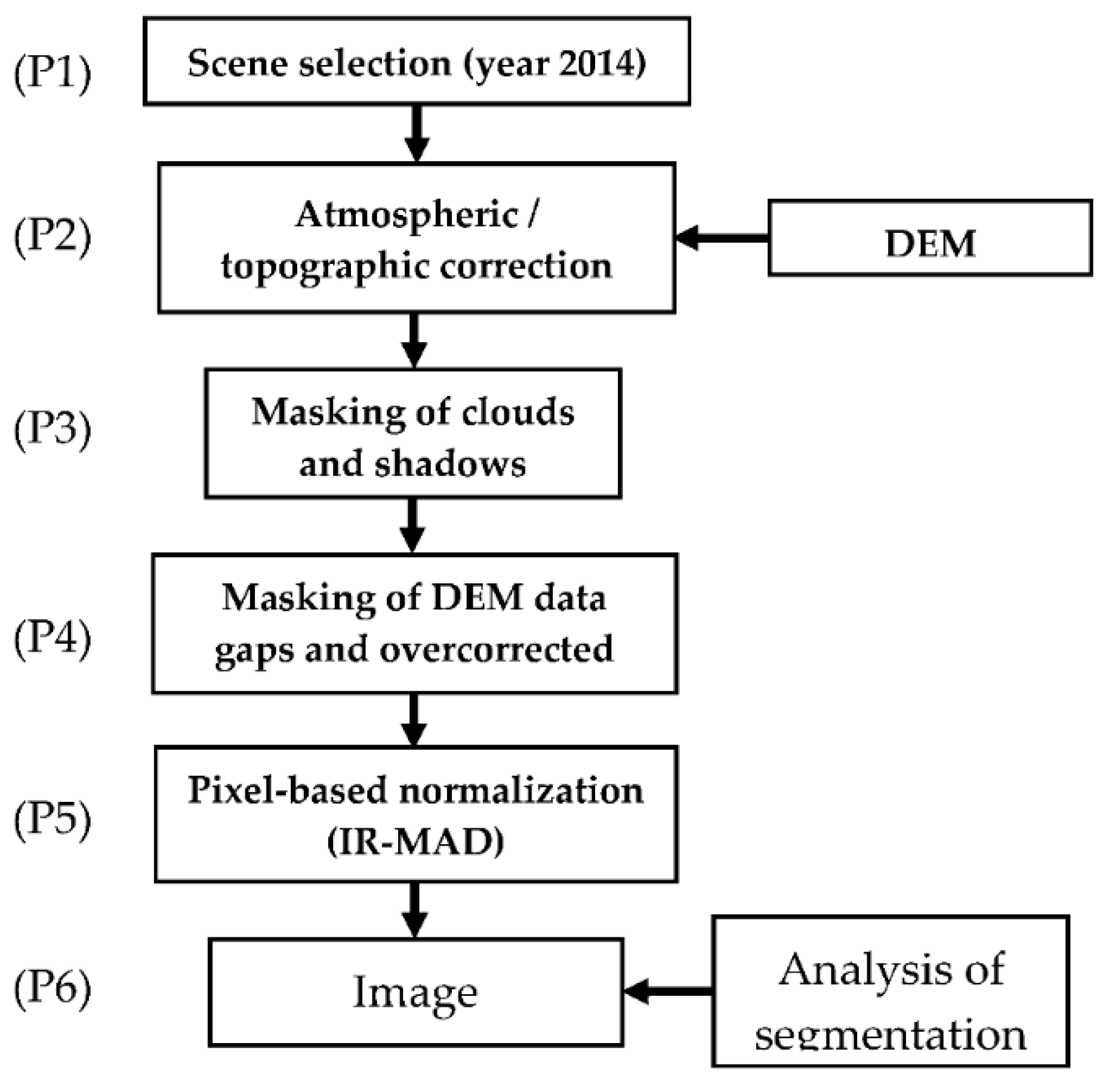
Figure 2 shows the flow of analysis. One problem with land cover mapping using remote sensing in mountainous terrain is the presence of sunlit and shadowed slopes produced by the steep topography. Topographic correction is necessary to reduce this effect.

After conducting atmospheric and topographic correction for the scenes (P2) and masking of clouds, cloud shadows, and pixels with overcorrected reflectance (P3 and P4), we normalized the satellite data. We conducted this process on pairs of overlapping scenes using the Iteratively Reweighted Multivariate Alteration Detection (IR-MAD) algorithm (P5) [21,22] to find pseudo-invariant features that can compute a modified model [23]. The size of sample areas was 10 km × 10 km, and the sample areas included deep water bodies, concrete, and/or bare soil, aside from forest areas. This method is based on canonical correlation analysis (CCA) and is an unsupervised change detection algorithm that is invariant to linear transformations of the original data. In this method, CCA creates linear combinations of the pixel values for each of the spectral bands of the two scenes. Each pair of linear combinations are called canonical variates (CVs), and the number of CVs is equal to the number of bands. The first pair of CVs has maximal correlation, the second pair of CVs has the second highest correlation and is orthogonal to the first pair of CVs, and so on. Then, the process to determine the difference between the CVs is carried out to produce a sequence of transformed difference images called MAD variates that records the maximum spread (or maximum change) of the pixel values. The sequence generates the same number of MAD variates as the number of bands used. From these different images, we select all pixels with minimum or no change (called Pseudo-Invariant Features, PIFs) that satisfy Formula (1):

$${{\displaystyle \sum }}_1^N{(\frac{MA{D}_i}{{\sigma }_{MA{D}_i}})}^2<t,$$

(1)

where N is the number of MAD variates, σ is the variance of the no-change distribution, and t is a decision threshold value. In the absence of change, the sum of the squares of standardized MAD variates is approximately chi-squared distributed with N degrees of freedom. The value of t is defined as:

$$t=X_{N,P=0.01}^2,$$

(2)

where P is the probability of observing a value lower than t. The process uses P as weight for the observations, and the whole process is iterated until a stopping criterion is met. In this study, we used a fixed number of iterations equal to 50. With this process, we selected PIFs to carry out linear regressions to produce linear equations for each band to normalize the reflectance values of the scenes. Finally, we created cloud-free normalized mosaics by overlapping the normalized scenes.

In contrast to pixel-based and unsupervised classification techniques, object-based image classification creates land cover maps that are easier to compare with reality. The object-based classification approach implies the creation of “objects” or “groups of pixels.” For this purpose, we carried out a series of a segmentation analyses using eCognition [24]. This process uses a region-merging algorithm starting with randomly selected pixel seeds that are distributed regularly [25]. The pixels are then grouped with other pixels based on the homogeneity criteria to form polygons called objects. By using a series of tests with different scale values and evaluating changes in the average size of the created objects, we determined an optimum segmentation scale value to produce objects with an average area equal to the minimum defined forest area (2 ha). Then, we segmented the cloud-free normalized mosaic with the optimum scale value (P6) to produce the objects we used in the classification analysis.

2.3.2. Training Datasets and Verification Datasets

Table 2 shows the land cover data collected by the field survey and through visual interpretation using the CE tool at the study site. Because of the highly fragmented land use (landscape) in the area, it was difficult to collect enough data on Andes mountain forest using CE to build a training dataset. Therefore, we redistributed the available land cover data records of the Andes mountain forest land to complete the training dataset to a percentage of at least 70% of the total data. As a result, we randomly redistributed the 45 combined land cover data records for Andes mountain forest into 33 data records (73%) for the training dataset and 12 (27%) data records for the verification dataset.

2.3.3. Classification Variables and Variable Selection

The values of the variables used in this study were obtained by an object-based analysis, which means that we used the values of the pixels within each object to calculate the value of the corresponding variable for each object and used the average value in our analyses. The raster datasets used were the cloud-free Landsat 8 OLI mosaic and STRM 30-m DEM data described in Table 1. Using the longitude and latitude of the land cover data records in the training and verification datasets, we determined the objects corresponding to each land cover point and then extracted the calculated value of the variables from those objects using the statistical software R version 3.4 (http://www.cran. R-project.org).

The average reflectance values of the visible bands (blue, green, and red), the near infrared (NIR) band, and two shortwave infrared bands were derived from the spectral data. Additionally, we used the three first principal components produced by principal component analysis and tasseled cap transformation, both of which reduce data dimensionality, taking into account the variability of the data as much as possible. We also used the Normalized Difference Vegetation Index (NDVI) and the Modified Soil-adjusted Vegetation Index (MSAVI). MSAVI was calculated as:

$$MSAVI=\frac{2\times {\rho }_{NIR}+1-\sqrt{{\left(2\times {\rho }_{NIR}+1\right)}^2-8\times \left({\rho }_{NIR}-{\rho }_{red}\right)}}{2},$$

(3)

where ρ_NIR and ρ_red are the reflectance values in the NIR and red bands, respectively. This index has been used in vegetation studies in arid and semi-arid regions [26,27,28] because it reduces the soil background effect. We chose to use it among other soil-adjusted vegetation indexes because it can be used without any preliminary knowledge of the vegetation cover rate [29].

We included elevation and aspect (the downward direction of the slope in degrees) calculated from the DEM data as topography-derived variables in the classification analysis, considering the ecological relationships between vegetation species, altitude, and slope orientation.

One of the characteristics of SVM and RF algorithms is that they do not require feature selection [30]. However, the performance of classifiers produced by kNN algorithm is affected by the presence of irrelevant or redundant features in the training data [31,32]. Since we wanted to determine which among these three machine learning algorithms can produce the most accurate classifier for Andes mountain forest classification, we chose to make such a comparison using the same models produced after feature selection and using the same subsets of data produced with cross validation. Additionally, in order to take into account the full capacity of the SVM and RF algorithms to produce highly accurate classifiers, we introduced and tested classifiers produced with all the available variables.

The variables were subjected to a selection process involving two analyses. In the first analysis, we determined the relative importance of the variables by using the Akaike weight [33], which is based on the Akaike information criterion (AIC), taking into account that our classification analysis had a binary outcome: Andes mountain forest or shrubland. To do this, we built models using all possible combination of the variables and calculated their corresponding AIC values. Then, we calculated the AIC difference (Δ_i) between each model (AIC_i) and the model with minimum AIC (AIC_min):

$${\Delta }_i=AI{C}_i-AI{C}_{min}.$$

(4)

If R is the total number of models, then the Akaike weight (w_i) can be calculated for each model as follows:

$$w_i=\frac{\exp \left(-\frac{1}{2}{\Delta }_i\right)}{{{\displaystyle \sum }}_{r=1}^R\exp \left(-\frac{1}{2}{\Delta }_r\right)}.$$

(5)

The relative importance of each variable was estimated by summing the Akaike weights of all the models in which the variable occurs. In the second analysis, we calculated the Pearson’s correlation coefficient between each pair of variables. We chose the variables with the higher values of relative importance and discarded the correlated variables with the lower importance value.

2.3.4. Classification Methods

RF is a powerful MLA that is widely used to classify imagery data for land cover classification using multispectral satellite sensor imagery. The method performs well when the number of predictors is greater than the number of observations and has low sensitivity when the number of irrelevant predictors is large. SVM is another MLA used for classification to determine a hyperplane (or boundary in a high dimensional space) that can divide training data into a predetermined number of categories. This method is used in many remote sensing studies because of its capacity to process small training datasets [34]. The kNN method is simple to implement and has a low training computational cost. This non-parametric method uses the k closest training data vectors to make predictions and has been used in forest inventory practices and as a tool for forest classification and mapping [35,36,37].

We carried out a comparative statistical analysis of the three MLAs using non-parametric statistical tests to compare the performances of all the considered models.

1. Random Forest

The RF method [38] is an ensemble of classification trees in which each tree contributes a unit vote to determine the most frequent class according to the input data (Equation (6)):

$$C_{rf}^m(x)=majorityvote{\left\{C_{m_i}(x)\right\}}_1^m,$$

(6)

where $C_{rf}^m(x)$ is the predicted class from the RF classification of data record x, and $C_{m_i}(x)$ is the predicted class from the classification tree m_i of the data record x. Each classification tree is constructed using a bootstrap sample of 63.2% of the training data, while the rest of the data is considered out-of-bag (OOB) data. When forming a split point (node) in a tree, the algorithm randomly selects a sub-set of variables and searches among these variables for the best split point to classify the data. The number of variables in each sub-set is commonly denoted as m_try. The performance of this algorithm depends on the availability of a sufficient number of trees (n_trees) to be generated to converge on the value of the OOB error and the number of variables randomly sampled as candidate variables in each node of the classification trees (m_try).

We used 4000 random decision trees. The OOB error is the average of the misclassification(s) rates computed from each sample of the OOB data when classified by all the trees constructed without such samples. We adjusted the value of m_try by carrying out a series of classification tests with different values of this parameter and calculated the corresponding Cohen’s kappa value. Then, we selected the value of m_try that had the maximum Cohen’s kappa value.

2. Support Vector Machine

SVM [39] is a non-parametric supervised statistical learning classifier that finds a hyperplane for optimal classification by minimizing the upper bound of the classification error. To use this method, we standardized the values of the variables in the training data. The method maximizes the distance from the data points of two classes (in the case of binary classification) to an optimal separation vector of a hyperplane created from the variables [40]. The hyperplane is the surface used to determine the classification.

Given a training set (x_i, y_i), where y_i is the class label that takes the value of –1 or 1 and x_i is the training vector of the values of the corresponding explanatory variables, a solution to the following optimization problem is needed:

$$\underset{\mathit{w},b,\xi }{\min } \frac{1}{2}{\mathit{w}}^T\mathit{w}+C{{\displaystyle \sum }}_{i=1}^l{\xi }_i,$$

(7)

$$\text{subject to }{y}_i\left({\mathit{w}}^T\varphi \left({\mathit{x}}_{\mathit{i}}\right)+\mathit{b}\right)\ge 1-{\xi }_i, {\xi }_i\ge 0,$$

(8)

where φ is a projection function of the training vector given by the kernel model used by the analyst; w and b are the adjustable weight and bias parameters, respectively; C is the penalty parameter of the error term ξ; l is the number of samples in the training dataset; and T denotes the transpose operator.

The parameters w and b in Equation (8) define the decision hyper-plane that separates the classes, and the minimization of Equation (7) aims to maximize the separation margin of the data. The projection function is related to a kernel function K by the following expression:

$$K\left({\mathit{x}}_{\mathit{i}},{\mathit{x}}_{{\mathit{i}}^{\prime }}\right)=\varphi \left({\mathit{x}}_{\mathit{i}}\right)·\varphi \left({\mathit{x}}_{{\mathit{i}}^{\prime }}\right)$$

(9)

We used the radial basis function kernel that depends on the value of the parameter γ in the following expression:

$$K\left({\mathit{x}}_{\mathit{i}},{\mathit{x}}_{{\mathit{i}}^{\prime }}\right)=exp\left(-\gamma {{\displaystyle \sum }}_{j=1}^p{\left({\mathit{x}}_{\mathit{i}\mathit{j}}-{\mathit{x}}_{{\mathit{i}}^{\prime }\mathit{j}}\right)}^2\right), \gamma >0.$$

(10)

where x_i and x_i’ are two different training vectors of the values of the explanatory variables; x_ij and x_i’j are the values of the jth explanatory variable in the ith and i’th training vectors; and p is the total number of variables. The parameter γ defines the extent to which the impact of a single training example extends to determine the decision surface. On the other hand, C trades off misclassification of training data against the number of dimensions that the decision surface should have. These two parameters were adjusted using a grid search analysis; that is, the best decision hyper-plane of the largest Cohen’s kappa value was calculated using different values of C and γ in a series of sequential tests.

3.k-Nearest Neighbors

kNN is a well-known nonparametric classification method that assigns a sample vector x to the class represented by the majority of k nearest neighbors whose similarity is determined by the distance measure. As with the SVM algorithm, the values of the variables in the training data need to be standardized to use this method. We used the Minkowski metric to define distance:

$$d(x_i,x_j)={\left({\displaystyle \sum _{s=1}^p{\left|x_{is}-x_{js}\right|}^q}\right)}^{1/q}$$

(11)

where x_i is the predictor vector of length p of observation i to be classified, and x_j is the jth nearest neighbor. Euclidean distances can be determined by setting the value of q = 2. When k_r is the number of nearest neighbors to the observation x_i that belongs to class r, then:

$${\displaystyle \sum _{r=1}^c{k}_r=k}.$$

(12)

The algorithm assigns observation x_i to the class r for which k_r is the largest. We restricted the value of k to odd values to avoid the possibility of a tie between the numbers of neighboring training data samples of two different classes. Because the performance of this method depends on the value of k, we adjusted its value by calculating the Cohen’s kappa value of a series of classification analyses using different values of the parameter and by choosing the value that had the maximum Cohen kappa value.

2.3.5. Tuning of Parameters and Performance Assessment of the Classification Models

We carried out a stratified 10-fold cross-validation using data corresponding to the classes “Andes mountain forests” and “shrubland,” dividing the data into 10 sub-datasets of approximately the same size and maintaining the ratio of data of each class. Each model was trained using nine folds of the data and validated with the remaining fold.

In order to avoid the overfitting problem, we followed a simple recommended approach to compare classifiers using cross-validation [41] by carrying out the classifier parameters’ tuning task using only the training data. The procedure is as follows:

• We created a training set T = A − k for each of the k subsets of the dataset A
• We divided the training set T into subsets t1 and t2; these subsets were used for training and tuning respectively. The subset of variables or features used to fine tune the classifiers are the same set of variables selected for each model, as shown in Section 3.1.
• When the parameters of the classifier were tuned for maximum accuracy, we re-ran each of the models with the initial larger training set T. We chose values of the tuning parameters that maximizes the average of Sensitivity and Specificity metrics. This criterion is recommended for conservation studies where omission error is undesirable [42].
• The classification precision indicators were calculated using the fold k as the validation data.
• Mean and standard deviation of the precision indicators were calculated for comparison analysis.

As performance indicators, we used Cohen’s kappa value and the area under the curve (AUC) from the receiver operating characteristic (ROC) theory [43,44]. Cohen’s kappa values were calculated using a confusion matrix constructed with the results obtained by classifying the verification data. However, because of the imbalance in the proportion of data between the two land cover types, the result was biased toward the larger one of the two. Thus, analyzing the performance of the models with a probability threshold of 0.5 will under-predict the occurrence of the rarest class [45,46]. To avoid this effect, we used the ROC curve to determine the corresponding optimum threshold of each classification analysis by selecting the threshold value that maximizes the average of Sensitivity and Specificity. Using the new calculated threshold value for each classification result in the cross-validation procedure, we constructed the corresponding confusion matrices from which Cohen’s kappa values were calculated. The AUC value is threshold independent, which means it gives a value of overall accuracy based on many different probability thresholds. The value of AUC varies from 0.5 to 1.0 (a perfect fit), and we calculated it with the R software package pROC.

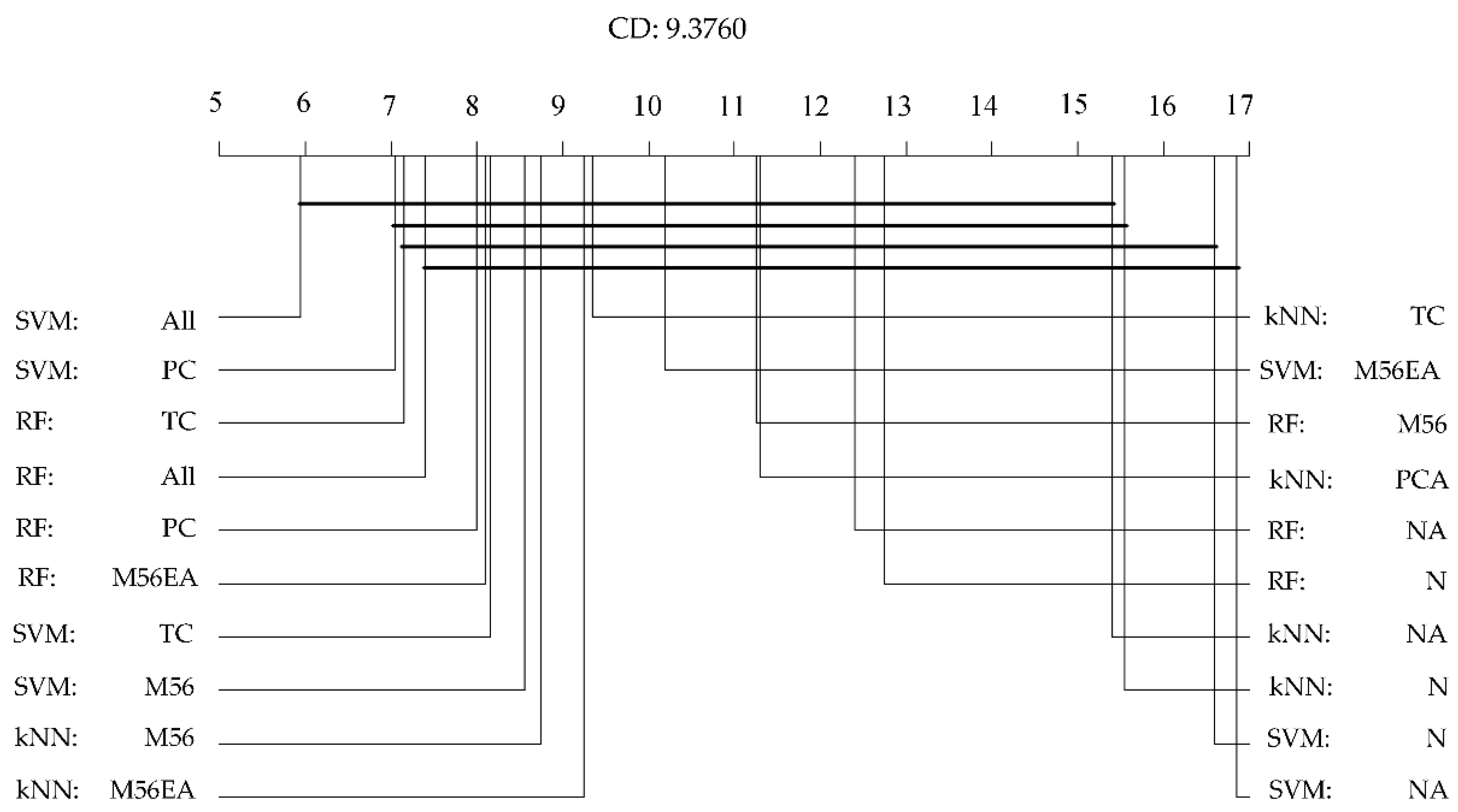
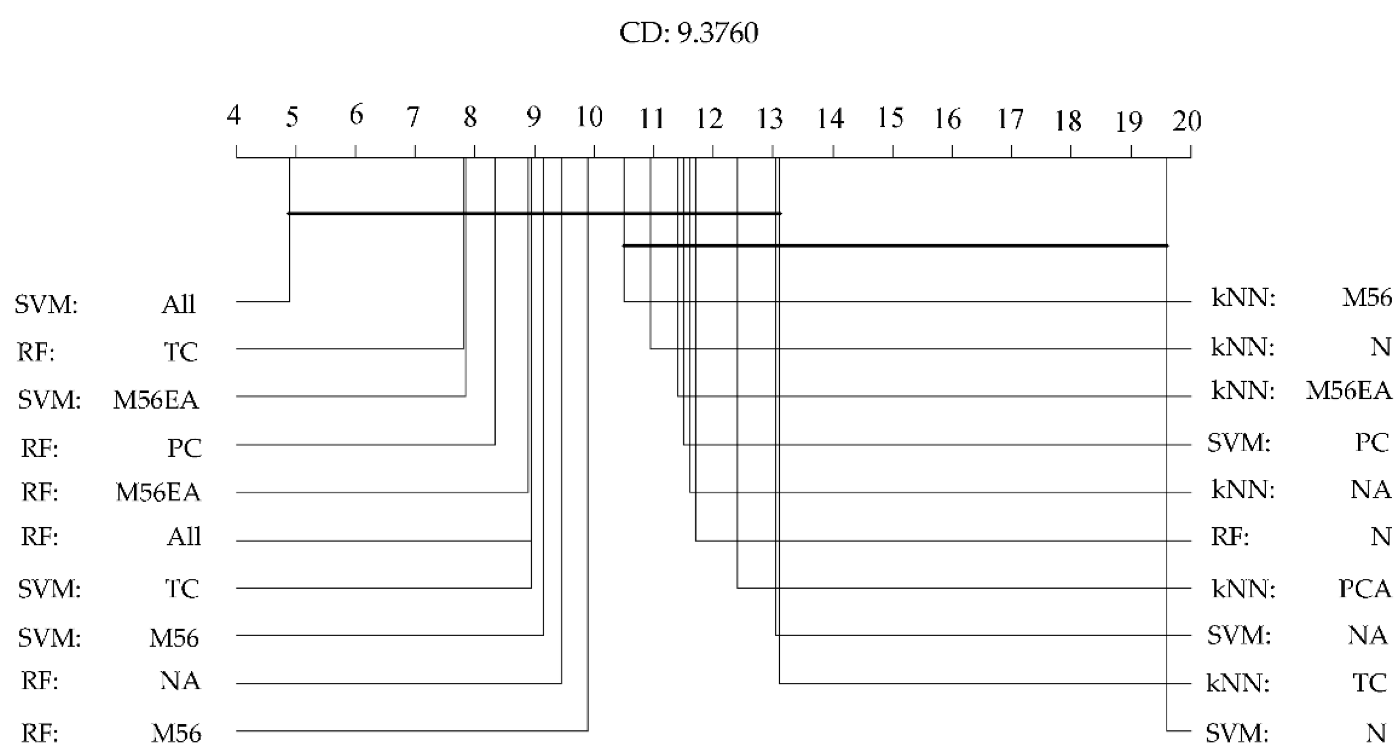
We ranked the performances of all of the models obtained with each fold and calculated the mean value of the ranks obtained per model [47]; a higher rank (1 being the highest rank) would indicate a higher performance indicator value. The mean ranks of the performance indicators were compared as well as the corresponding mean and standard deviation. Also, Friedman tests were carried out to determine if the various models yielded statistically different AUC and Cohen’s kappa values [48]. The test was conducted using the mean rank of the performances of all of the models. If the p-value of the test was significant (p < 0.05), we could reject the null hypothesis that the difference in classification performances between the models is zero. Then, using the Nemenyi post-hoc test, we carried out a pairwise multiple comparison of ranks and determined which models show a significant performance difference compared to the others by using the critical distance (CD) [49]. This test is conservative and robust when analyzing a small amount of unbalanced data. The CD value was calculated as follows:

$$CD=q_{\alpha }\sqrt{\frac{k\left(k + 1\right)}{6N}},$$

(13)

where N is the number of folds, k is the number of models to be compared, α is the confidence level, and q_α is the critical value based on the Studentized range statistic that depends on the significance level α and k.

Finally, we attempted to determine if, given the same set of variables, a particular MLA would produce a better classifier for “Andes mountain forest” vs. “shrubs” classification. For this, we conducted Nemenyi post-hoc statistical tests to test to determine if there is a significant difference between the performance indicator values of a particular model produced by RF, SVM, and kNN.

3. Results

3.1. Selection of Variables and Constructed Models

Table 3. Total sum of the Akaike weights for the variables in the study. Higher values indicate greater importance.

Variable	Elev.	MSAVI	B5	NDVI	Aspect
Total AIC weight	0.88	0.81	0.80	0.62	0.58
Variable	B6	B7	B2	B3	B4
Total AIC weight	0.53	0.48	0.46	0.43	0.37

Elev.: elevation; NDVI: normalized difference vegetation index; MSAVI: modified soil-adjusted vegetation index; B2, B3, B4, B5, B6, and B7: mean reflectance values of bands 2, 3, 4, 5, 6 and 7 of the Landsat 8 OLI scene.

shows the total Akaike weights used to rank the variables in order of importance to differentiate Andes mountain forest and shrubland. The most important variables are the mean values of elevation, MSAVI, and the reflectance in the NIR band (B5 in Table 1).

Table 4. Pearson correlation matrix for the variables in the study. Significant low correlation values are shaded.

	B2	B3	B4	B5	B6	B7	NDVI	MSAVI	Elev.
B2
B3	0.97 ***
B4	0.93 ***	0.96 ***
B5	0.00	0.11 ***	−0.05 ***
B6	0.51 ***	0.58 ***	0.62 ***	0.04 ***
B7	0.62 ***	0.67 ***	0.73 ***	−0.11 ***	0.95 ***
NDVI	−0.70 ***	−0.69 ***	−0.81 ***	0.51 ***	−0.51 ***	−0.67 ***
MSAVI	−0.39 ***	−0.38 ***	−0.43 ***	0.34 ***	−0.22 ***	−0.32 ***	0.65 ***
Elev.	0.44 ***	0.44 ***	0.57 ***	−0.44 ***	0.43 ***	0.53 ***	−0.69 ***	−0.34 ***
Asp.	0.06 ***	0.06 ***	0.05 ***	0.05 ***	0.13***	0.10***	−0.02 ***	−0.01 ***	0.02 ***

*** p < 0.001.

shows the matrix of Pearson correlations. With the exception of the mean reflectance of Band 5, all of the mean reflectance values of the Landsat 8 OLI bands are correlated with each other. Elevation has a strong negative correlation with NDVI, which reflects a decrease in green vegetation mass along the altitude gradient observed during the field surveys. Although NDVI is correlated with all variables except aspect, MSAVI was only correlated with NDVI. Elevation also showed a high correlation with the mean reflectance of short wavelength infrared 2 (B7). Since Elevation showed a higher Total AIC value, Elevation was preferred over B7.

Using Table 3 and Table 4, we chose uncorrelated variables of great importance to build models that contained one vegetation index. We also included the same models without the topographic variables to test whether the model accuracy increased when these variables were included. Following these criteria, we built models with the following features:

• M56EA: MSAVI, Band 5, Band 6, elevation, and aspect
• M56: MSAVI, Band 5, and Band 6
• NA: NDVI and aspect
• N: NDVI
• PC: Principal components 1, 2, and 3
• TC: Tasseled cap bands 1, 2, and 3

We also compared models produced by the SVM and RF algorithms using all the variables available: mean reflectance from the bands 2 to 7, NDVI, MSAVI, and mean values of elevation and topographic aspect. These models were denoted as SVM:All and RF:All.

3.2. AUC and Cohen’s Kappa Results

Table 5. Models ranked by AUC values obtained by 10-fold cross-validation.

MLA:Model	Mean Rank	Mean	SD	BCI 2.5%	BCI 97.5%
SVM:All	5.9	0.81	0.10	0.75	0.85
SVM:PC	7.1	0.78	0.11	0.72	0.85
RF:TC	7.2	0.79	0.11	0.73	0.86
RF:All	7.4	0.79	0.11	0.72	0.84
RF:PC	8.0	0.78	0.11	0.70	0.84
RF:M56EA	8.1	0.78	0.10	0.71	0.83
SVM:TC	8.2	0.77	0.11	0.71	0.85
SVM:M56	8.6	0.76	0.12	0.69	0.84
kNN:M56	8.8	0.75	0.15	0.65	0.82
kNN:M56EA	9.3	0.75	0.08	0.71	0.81
kNN:TC	9.4	0.75	0.10	0.69	0.81
SVM:M56EA	10.2	0.73	0.14	0.65	0.81
RF:M56	11.3	0.72	0.14	0.64	0.79
kNN:PC	11.3	0.73	0.10	0.67	0.79
RF:NA	12.4	0.70	0.08	0.65	0.74
RF:N	12.8	0.69	0.07	0.65	0.73
kNN:NA	15.4	0.63	0.11	0.56	0.69
kNN:N	15.6	0.65	0.10	0.59	0.71
SVM:N	16.6	0.52	0.20	0.42	0.65
SVM:NA	16.9	0.61	0.12	0.55	0.69

SD: standard deviation; BCI: bootstrap confidence interval calculated by bootstrap analysis with 1000 repetitions.

and

Table 6. Models ranked by Cohen’s kappa values obtained by 10-fold cross-validation.

MLA:Model	Mean Rank	Mean	SD	BCI 2.5%	BCI 97.5%
SVM:All	4.9	0.43	0.13	0.37	0.53
RF:TC	7.8	0.35	0.17	0.28	0.48
SVM:M56EA	7.9	0.36	0.20	0.26	0.48
RF:PC	8.4	0.32	0.11	0.26	0.38
RF:M56EA	8.9	0.33	0.12	0.26	0.42
RF:All	9.0	0.32	0.12	0.25	0.39
SVM:TC	9.0	0.35	0.22	0.26	0.56
SVM:M56	9.2	0.32	0.13	0.25	0.40
RF:NA	9.5	0.31	0.14	0.21	0.38
RF:M56	9.9	0.29	0.18	0.19	0.41
kNN:M56	10.5	0.29	0.09	0.24	0.35
kNN:N	11.0	0.30	0.20	0.18	0.42
kNN:M56EA	11.4	0.29	0.15	0.22	0.41
SVM:PC	11.5	0.27	0.15	0.20	0.40
kNN:NA	11.6	0.26	0.11	0.21	0.36
RF:N	11.7	0.26	0.12	0.16	0.32
kNN:PC	12.4	0.25	0.10	0.20	0.33
SVM:NA	13.1	0.22	0.16	0.13	0.31
kNN:TC	13.1	0.24	0.08	0.19	0.28
SVM:N	19.6	0.03	0.03	0.02	0.06

SD: standard deviation; BCI: bootstrap confidence interval calculated by bootstrap analysis with 1000 repetitions.

show the mean rank calculated for all the models using AUC and Cohen’s kappa values, respectively, obtained by the 10-fold cross-validation procedure.

We can observe that the model with the highest AUC and Cohen’s Kappa mean values was produced by the SVM algorithm: SVM:All. In contrast, SVM:N and SVM:NA had the lowest mean values of the performance indicators. This result suggests that the performance of a classifier produced by the SVM algorithm is highly related to the dimensionality of the training dataset.

3.3. Non-Parametric Tests for Multiple Comparisons

The Friedman test results showed a significant difference in the AUC (Χ² = 62.29, df = 19, p = 1.7 × 10⁻⁶) and Cohen’s kappa (Χ² = 47.46, df = 19, p = 3.1 × 10⁻⁴) values of all the models. This indicates that at least one model has different performance values (i.e., it is safe to reject the null hypothesis that all the classification models perform the same). Therefore, we could proceed with the Nemenyi post-hoc test.

We carried out the comparative analysis of all of the models using the mean rank calculated using AUC and Cohen’s kappa values. Using the calculated value of CD = 9.3760, we connected the groups of models that have statistically similar values of performance indicators (Figure 3 and Figure 4). For the AUC test (Figure 3), only the distance between the rank of the worst model (SVM:NA) and the three best models (SVM:All, SVM:PC, and RF:TC) were greater than the CD value. This indicates that these three models performed significantly better than the rest, and that the models SVM:NA, SVM:N, and kNN:N are, statistically, the worst performing models. We also noticed that the model produced by the kNN method with the highest mean value of performance indicators (kNN:M56, AUC = 0.75, Cohen’s Kappa = 0.29) and the worst performing models belong to the same group determined by CD. On the other hand, the models produced by the SVM and RF methods with the highest mean value of performance indicators (SVM:All, AUC = 0.81, Cohen’s Kappa = 0.43; RF:TC, AUC = 0.79, Cohen’s Kappa = 0.35) showed no significant difference.

The Cohen’s kappa value comparison (Figure 4) shows that the model SVM:All and other nine models have mean Cohen’s kappa values that are statistically different from the worst performing model: SVM:N. However, the only model with a kappa value high enough to reach moderate agreement (>0.4) is SVM:All.

Table 7. p values of the Nemenyi post-hoc tests for multiple comparisons. The table shows the p values resulting from the pairwise comparisons of AUC values produced by classifiers using the same variables but produced by different MLAs. No significant differences (p < 0.05) are observed.

Model 1: M56EA			Model 2: M56
	kNN	SVM		kNN	SVM
SVM	0.97	–	SVM	0.64	–
RF	0.90	0.97	RF	0.97	0.50
Model 3: NA			Model 4: N
	kNN	SVM		kNN	SVM
SVM	0.90	–	SVM	0.64	–
RF	0.50	0.26	RF	0.64	0.17
Model 5: PC			Model 6: TC
	kNN	SVM		kNN	SVM
SVM	0.26	–	SVM	0.37	–
RF	0.17	0.97	RF	0.78	0.78

and

Table 8. p values of the Nemenyi post-hoc tests for multiple comparisons. The table shows the p values resulting from the pairwise comparisons of Cohen’s Kappa values produced by classifiers using the same variables but produced by different MLAs. Significant differences (p < 0.05) are underlined.

Model 1: M56EA			Model 2: M56
	kNN	SVM		kNN	SVM
SVM	0.17	–	SVM	0.97	–
RF	0.64	0.64	RF	0.64	0.50
Model 3: NA			Model 4: N
	kNN	SVM		kNN	SVM
SVM	0.94	–	SVM	0.02	–
RF	0.57	0.37	RF	1.0	0.02
Model 5: PC			Model 6: TC
	kNN	SVM		kNN	SVM
SVM	0.261	–	SVM	0.173	–
RF	0.037	0.644	RF	0.065	0.896

show the results of the Nemenyi test for pairwise comparison of the classification performance of machine learning algorithms per model using AUC and Cohen’s kappa as the performance indicator, respectively. The test shows a significant difference in Cohen’s kappa value in only three cases. In one case, it shows that RF can generate a better performing classifier than kNN when using principal components. In the other two cases, it shows that the RF and kNN algorithms can produce a classifier for Andes mountain forests with a kappa value significantly higher than the SVM algorithm when using the NDVI as the only classification feature.

4. Discussion

4.1. Aspects of Land Cover Classification in the Andes Mountain Region

The Andes region has a complex topography. Its altitudinal range yields an environmental gradient that contains a variety of ecosystems, vegetation communities, and forest formations. Human pressure on the Andes mountains puts natural resources such as its mountain forests at risk. The evaluation and monitoring of forest conditions is very important for conservation activities and land cover mapping is one important tool to accomplish them. Remote sensing is widely used to monitor large areas at relatively low cost and produce the necessary maps for forest monitoring. This study provides an important contribution on the selection of better classification techniques to create more accurate maps for Andes mountain forests.

Mapping and monitoring large areas of vegetation in semi-arid environments using remote sensing techniques is challenging. One issue is the collection of good quality training data, because the terrain and mixed vegetation introduce noise to the data [50]. Such is the case for the Andes mountain terrain, and its remaining low-density forest consisting of a mixed population of native tree species and shrubs. Hence, robust classification methods are essential for mapping this type of forest. Well-known parametric methods such as the maximum likelihood method (ML) have been used for forest mapping using remote sensing data, as well as more complex non-parametric algorithms such as RF, SVM, and kNN which, unlike ML, do not require prior knowledge of the underlying probability density function. In particular, RF and SVM have been shown to outperform ML because they can handle large multivariate and highly collinear datasets [51], which are provided by multispectral (e.g., LANDSAT, SPOT) and newer hyperspectral (e.g., AVIRIS, EO-1Hyperion) high resolution imagery.

When sampling data from a rare land cover type, it is necessary to select a sampling method that enables statistically robust comparisons and logistically feasible sampling within the available budget and staff capacity. However, classification analysis using machine learning algorithms is only as effective as the quality and quantity of the training data they are learning from. We combined an exhaustive field survey within the study area and an indirect sampling method to gather enough data to cover the reflectance variability of Andes mountain forest within the study region (Cuzco, Peru). For this reason, the direct application of these results is restricted to a region of the Andes where forest communities with the same species composition and vegetation structure exist. Given our data collection strategy, we were able to identify models that have the highest and lowest classification performance by using a conservative statistical test (significance level = 5%).

4.2. Comparison of MLA Classifiers

By comparing the performances of classifiers produced by the same machine learning algorithm (MLA) in Table 5 and Table 6, we observed higher performances in models using the Modified Soil-adjusted Vegetation Index rather than the Normalized Difference Vegetation Index. This can be explained by the effect of soil brightness over the NIR-red band ratio [52], which affects NDVI. On the other hand, MSAVI is less sensitive to changes in soil brightness (due to soil background variations) and shadows than NDVI. This suggests that MSAVI could be a better variable to classify different vegetation types in arid and semi-arid regions where the vegetation cover rate is low. Also, the model SVM:All shows the highest mean AUC and Cohen’s kappa values, which suggests that SVM:All is the best model for classifying Andes mountain forests and shrubland.

The results of this research provide new insights to the performance of RF, SVM, and kNN algorithms in the context of mapping Andean forests over large areas with noisy data. Table 5 and Figure 3 show that only three models with the highest ranks have a statistically better performance than the lowest ranked model (SVM:NA), whereas the classification performances of the remaining models were not statistically different. One way to choose from these three top-performing models is to examine the performance indicator’s standard deviation. Of the three best models, SVM:All had the highest mean AUC value and the smallest standard deviation followed by SVM:PC which uses a transformation to reduce the dimensionality of the training data used by the former. When analyzing the Cohen’s Kappa values (Table 6 and Figure 4) there are ten models that statistically out-perform the worst model. It should be noted that none of these ten models were generated using the kNN algorithm. The performance of kNN was low compared with the other methods, probably because kNN has a greater reliance on data quality. Since this algorithm determines similarity by using the minimum distance to the reference data, the performance of the algorithm is very sensitive to the presence of outliers and noise in the data that was selected to train the classifier. Since Andes mountain forest land cover data is inherently noisy, SVM and RF are more suitable methods for mapping this type of terrain.

4.3. The Kappa Coefficient and Its Use as a Performance Indicator of Classification Models

This paper used the area under the curve (AUC) and the Cohen’s kappa coefficient for performance assessment of the MLAs. In particular, the Cohen’s kappa coefficient is a measure that takes into account the possibility of agreement by chance, and variations of it have been proposed to improve it [53]. Its use has been met with intense discussion; for example, Pontius and Millones [54] pointed out that Cohen’s kappa coefficient masks sources of error that are significantly different, and its dependence on a comparison with chance agreement is not informative. Although other authors have also criticized this indicator [55,56,57,58], to this day, Cohen’s kappa value is still a widely used metric in remote sensing to report classification results [59,60,61,62,63]. For this reason, we recommend using additional performance indicators to be used in conjunction with Cohen’s kappa value.

4.4. Machine Learning Algorithms and Contrast to Recent Research

Machine learning algorithms and their applications, such as regression and classification, have been studied for many years. These applications depend on estimating the probability distribution of the population data from samples, which is the most fundamental statistical approach [64]. A simpler approach called density-ratio estimation involves estimating the ratio of probability densities instead of the probability distribution. Density-ratio estimation has been used for predicting forest stand attributes [65] and land cover detection [66], and its application in a framework of machine learning has been proposed [67,68]. Future research should focus on deepening the application of this new framework for probabilistic classification and determining whether or not this approach produces more accurate results in the classification of mountain forests when using noisy data.

5. Conclusions

In this study, we determined the best model to classify Andes mountain forests and shrubland through a series of statistical comparisons using Landsat 8 OLI satellite data and land cover data. We concluded that the highest classification performance was obtained from a SVM classification model using the reflectance values from bands 2 to 7, NDVI, MSAVI, and the topographic variables elevation and aspect.

Based on our statistical pairwise comparison of the MLAs per model (Table 7 and Table 8), we found that the SVM and RF algorithm produce comparable classifiers for distinguishing Andes mountain forests and shrub land.

In contrast, the kNN models generally yielded lower ranks and lower mean values of performance indicators when compared with the SVM and RF models. These results suggest that the kNN algorithm had the lowest performance in the comparison test. One possible reason is that kNN is a “lazy learner”; that is, this method does not create classification rules from training data that can be generalized when classifying new data. Instead, it uses the training data (itself) to carry out the classification and predicts the class label of the new data from the k closest neighbors. This approach is likely to be a problem in classifying noisy training data which are derived from the variability of reflectance values in sparse Andes mountain forests that commonly grow in association with shrubland.

In conclusion, the results of our statistical analyses suggest that SVM and RF are suitable machine learning methods for producing accurate classifier for Andes mountain forests.

References

1. Zutta, B.R.; Rundel, P.W.; Saatchi, S.; Casana, J.D.; Gauthier, P.G.; Soto, A.; Velazco, Y.; Buermann, W. Prediciendo la distribución de Polylepis: Bosques Andinos vulnerables y cada vez más importantes. Rev. Peru. Biol. 2012, 19. [Google Scholar] [CrossRef]
2. Fjeldså, J.; Kessler, M.; Engblom, G.; Driesch, P. Conserving the Biological Diversity of Polylepis Woodlands of the Highland of Peru and Bolivia: A Contribution to Sustainable Natural Resource Management in the Andes; NORDECO: Copenhagen, Denmark, 1996; ISBN 978-87-986168-0-1. [Google Scholar]
3. Kessler, M. The “Polylepis problem“: Where do we stand? Ecotropica 2002, 8, 97–110. [Google Scholar]
4. Servat Grace, P.; Mendoza, C.W.; Ochoa, C.J.A. Flora y fauna de cuatro bosques de Polylepis (Rosaceae) en la Cordillera del Vilcanota (Cusco, Perú). Ecol. Appl. 2002, 1, 25–35. [Google Scholar] [CrossRef]
5. Roberts, D.A.; Gardner, M.; Church, R.; Ustin, S.; Scheer, G.; Green, R.O. Mapping Chaparral in the Santa Monica Mountains Using Multiple Endmember Spectral Mixture Models. Remote Sens. Environ. 1998, 65, 267–279. [Google Scholar] [CrossRef]
6. Smith, M.O.; Ustin, S.L.; Adams, J.B.; Gillespie, A.R. Vegetation in deserts: I. A regional measure of abundance from multispectral images. Remote Sens. Environ. 1990, 31, 1–26. [Google Scholar] [CrossRef]
7. Byambakhuu, I.; Sugita, M.; Matsushima, D. Spectral unmixing model to assess land cover fractions in Mongolian steppe regions. Remote Sens. Environ. 2010, 114, 2361–2372. [Google Scholar] [CrossRef] [Green Version]
8. Song, C. Spectral mixture analysis for subpixel vegetation fractions in the urban environment: How to incorporate endmember variability? Remote Sens. Environ. 2005, 95, 248–263. [Google Scholar] [CrossRef]
9. Meyer, P.; Itten, K.I.; Kellenberger, T.; Sandmeier, S.; Sandmeier, R. Radiometric corrections of topographically induced effects on Landsat TM data in an alpine environment. ISPRS J. Photogramm. Remote Sens. 1993, 48, 17–28. [Google Scholar] [CrossRef]
10. Li, M.; Im, J.; Beier, C. Machine learning approaches for forest classification and change analysis using multi-temporal Landsat TM images over Huntington Wildlife Forest. GISci. Remote Sens. 2013, 50, 361–384. [Google Scholar] [CrossRef]
11. Duro, D.C.; Franklin, S.E.; Dubé, M.G. A comparison of pixel-based and object-based image analysis with selected machine learning algorithms for the classification of agricultural landscapes using SPOT-5 HRG imagery. Remote Sens. Environ. 2012, 118, 259–272. [Google Scholar] [CrossRef]
12. Lu, D.; Weng, Q. A survey of image classification methods and techniques for improving classification performance. Int. J. Remote Sens. 2007, 28, 823–870. [Google Scholar] [CrossRef]
13. Paneque-Gálvez, J.; Mas, J.-F.; Moré, G.; Cristóbal, J.; Orta-Martínez, M.; Luz, A.C.; Guèze, M.; Macía, M.J.; Reyes-García, V. Enhanced land use/cover classification of heterogeneous tropical landscapes using support vector machines and textural homogeneity. Int. J. Appl. Earth Observ. Geoinf. 2013, 23, 372–383. [Google Scholar] [CrossRef]
14. Asner, G.P. Tropical forest carbon assessment: Integrating satellite and airborne mapping approaches. Environ. Res. Lett. 2009, 4, 034009. [Google Scholar] [CrossRef]
15. Potapov, P.V.; Dempewolf, J.; Talero, Y.; Hansen, M.C.; Stehman, S.V.; Vargas, C.; Rojas, E.J.; Castillo, D.; Mendoza, E.; Calderón, A.; et al. National satellite-based humid tropical forest change assessment in Peru in support of REDD+ implementation. Environ. Res. Lett. 2014, 9, 124012. [Google Scholar] [CrossRef]
16. Bader, M.Y.; Ruijten, J.J.A. A topography-based model of forest cover at the alpine tree line in the tropical Andes. J. Biogeogr. 2008, 35, 711–723. [Google Scholar] [CrossRef]
17. Gottlicher, D.; Obregon, A.; Homeier, J.; Rollenbeck, R.; Nauss, T.; Bendix, J. Land-cover Classification in the Andes of Southern Ecuador Using Landsat ETM+ Data As a Basis for SVAT Modelling. Int. J. Remote Sens. 2009, 30, 1867–1886. [Google Scholar] [CrossRef]
18. Josse, C.; Cuesta, F.; Navarro, G.; Barrena, V.; Cabrera, E.; Chacón-Moreno, E.; Ferreira, W.; Peralvo, M.; Tovar, A.S.J. Ecosistemas de los Andes del Norte y Centro. Bolivia, Colombia, Ecuador, Perú y Venezuela; Secretaría General de la Comunidad Andina: Lima, Peru, 2009; ISBN 978-9972-787-77-5. [Google Scholar]
19. Ministerio del Ambiente. Mapa Nacional de Cobertura Vegetal: Memoria Descriptiva; Dirección General de Evaluación, Valoración y Financiamiento del Patrimonio Natural, MINAM: Lima, Peru, 2015.
20. Ansión, J. El Árbol y el Bosque en la Sociedad Andina; Proyecto FAO/Holanda/INFOR: Lima, Peru, 1986. [Google Scholar]
21. Nielsen, A.A.; Conradsen, K.; Simpson, J.J. Multivariate Alteration Detection (MAD) and MAF Postprocessing in Multispectral, Bitemporal Image Data: New Approaches to Change Detection Studies. Remote Sens. Environ. 1998, 64, 1–19. [Google Scholar] [CrossRef]
22. Nielsen, A.A. The Regularized Iteratively Reweighted MAD Method for Change Detection in Multi- and Hyperspectral Data. IEEE Trans. Image Process. 2007, 16, 463–478. [Google Scholar] [CrossRef] [PubMed] [Green Version]
23. Canty, M.J.; Nielsen, A.A. Automatic radiometric normalization of multitemporal satellite imagery with the iteratively re-weighted MAD transformation. Remote Sens. Environ. 2008, 112, 1025–1036. [Google Scholar] [CrossRef]
24. eCognition eCognition Developer|Trimble. Available online: http://www.ecognition.com/suite/ecognition-developer (accessed on 2 October 2017).
25. Baatz, M.; Schäpe, A. Multiresolution Segmentation: An Optimization Approach for High Quality Multi-Scale Image Segmentation; Strobl, J., Blaschke, T., Griesebener, G., Eds.; Herbert Wichmann Verlag: Salzburg, Austria, 2000; pp. 12–23. [Google Scholar]
26. Rondeaux, G.; Steven, M.; Baret, F. Optimization of soil-adjusted vegetation indices. Remote Sens. Environ. 1996, 55, 95–107. [Google Scholar] [CrossRef]
27. Leprieur, C.; Kerr, Y.H.; Mastorchio, S.; Meunier, J.C. Monitoring vegetation cover across semi-arid regions: Comparison of remote observations from various scales. Int. J. Remote Sens. 2000, 21, 281–300. [Google Scholar] [CrossRef]
28. Schmidt, H.; Karnieli, A. Sensitivity of vegetation indices to substrate brightness in hyper-arid environment: The Makhtesh Ramon Crater (Israel) case study. Int. J. Remote Sens. 2001, 22, 3503–3520. [Google Scholar] [CrossRef]
29. Qi, J.; Chehbouni, A.; Huete, A.R.; Kerr, Y.H.; Sorooshian, S. A modified soil adjusted vegetation index. Remote Sens. Environ. 1994, 48, 119–126. [Google Scholar] [CrossRef]
30. Melgani, F.; Bruzzone, L. Classification of hyperspectral remote sensing images with support vector machines. IEEE Trans. Geosci. Remote Sens. 2004, 42, 1778–1790. [Google Scholar] [CrossRef]
31. Andrew Hall, M. Correlation-Based Feature Selection for Machine Learning; University of Waikato: Hamilton, New Zealand, 1999. [Google Scholar]
32. Huang, S.H. Supervised feature selection: A tutorial. Artif. Intell. Res. 2015, 4, 22. [Google Scholar] [CrossRef]
33. Burnham, K.P.; Anderson, D.R. Model Selection and Multimodel Inference: A Practical Information-Theoretic Approach, 2nd ed.; Springer: New York, NY, USA, 2010; ISBN 978-0-387-22456-5. [Google Scholar]
34. Mountrakis, G.; Im, J.; Ogole, C. Support vector machines in remote sensing: A review. ISPRS J. Photogramm. Remote Sens. 2011, 66, 247–259. [Google Scholar] [CrossRef]
35. Haapanen, R.; Ek, A.R.; Bauer, M.E.; Finley, A.O. Delineation of forest/nonforest land use classes using nearest neighbor methods. Remote Sens. Environ. 2004, 89, 265–271. [Google Scholar] [CrossRef]
36. Franco-Lopez, H.; Ek, A.R.; Bauer, M.E. Estimation and mapping of forest stand density, volume, and cover type using the k-nearest neighbors method. Remote Sens. Environ. 2001, 77, 251–274. [Google Scholar] [CrossRef]
37. McRoberts, R.E.; Nelson, M.D.; Wendt, D.G. Stratified estimation of forest area using satellite imagery, inventory data, and the k-Nearest Neighbors technique. Remote Sens. Environ. 2002, 82, 457–468. [Google Scholar] [CrossRef]
38. Breiman, L. Random Forests. Mach. Learn. 2001, 45, 5–32. [Google Scholar] [CrossRef]
39. Cortes, C.; Vapnik, V. Support-vector networks. Mach. Learn. 1995, 20, 273–297. [Google Scholar] [CrossRef]
40. Petropoulos, G.P.; Kalaitzidis, C.; Prasad Vadrevu, K. Support vector machines and object-based classification for obtaining land-use/cover cartography from Hyperion hyperspectral imagery. Comput. Geosci. 2012, 41, 99–107. [Google Scholar] [CrossRef]
41. Salzberg, S.L. On Comparing Classifiers: Pitfalls to Avoid and a Recommended Approach. Data Min. Knowl. Discov. 1997, 1, 317–328. [Google Scholar] [CrossRef]
42. Jiménez-Valverde, A.; Lobo, J.M. Threshold criteria for conversion of probability of species presence to either-or presence-absence. Acta Oecol. 2007, 31, 361–369. [Google Scholar] [CrossRef]
43. Metz, C.E. Basic principles of ROC analysis. Semin. Nucl. Med. 1978, 8, 283–298. [Google Scholar] [CrossRef]
44. Hanley, J.A.; McNeil, B.J. The meaning and use of the area under a receiver operating characteristic (ROC) curve. Radiology 1982, 143, 29–36. [Google Scholar] [CrossRef] [PubMed]
45. Liu, C.; Berry, P.M.; Dawson, T.P.; Pearson, R.G. Selecting thresholds of occurrence in the prediction of species distributions. Ecography 2005, 28, 385–393. [Google Scholar] [CrossRef]
46. Freeman, E.A.; Moisen, G.G. A comparison of the performance of threshold criteria for binary classification in terms of predicted prevalence and kappa. Ecol. Model. 2008, 217, 48–58. [Google Scholar] [CrossRef]
47. Demšar, J. Statistical Comparisons of Classifiers over Multiple Data Sets. J. Mach. Learn. Res. 2006, 7, 1–30. [Google Scholar]
48. Friedman, M. The Use of Ranks to Avoid the Assumption of Normality Implicit in the Analysis of Variance. J. Am. Stat. Assoc. 1937, 32, 675–701. [Google Scholar] [CrossRef]
49. Nemenyi, P. Distribution-Free Multiple Comparisons. Ph.D. Thesis, Princeton University: Princeton, NJ, USA, 1963. [Google Scholar]
50. Ringrose, S.; Matheson, W.; Mogotsi, B.; Tempest, F. Nature of the darkening effect in drought affected savannah woodland environments relative to soil reflectance in Landsat and Spot Wavebands. Remote Sens. Environ. 1989, 25, 519–524. [Google Scholar]
51. Nitze, I.; Schulthess, U.; Asche, H. Comparison of machine learning algorithms random forest, artificial neural network and support vector machine to maximum likelihood for supervised crop type classification. In Proceedings of the 4th international conference on Geographic Object-Based Image Analysis (GEOBIA) Conference; Rio de Janeiro, Brazil, 7–9 May 2012; pp. 35–40. [Google Scholar]
52. Huete, A.R.; Jackson, R.D.; Post, D.F. Spectral response of a plant canopy with different soil backgrounds. Remote Sens. Environ. 1985, 17, 37–53. [Google Scholar] [CrossRef]
53. Stein, A.; Aryal, J.; Gort, G. Use of the Bradley-Terry model to quantify association in remotely sensed images. IEEE Trans. Geosci. Remote Sens. 2005, 43, 852–856. [Google Scholar] [CrossRef]
54. Pontius, R.G.; Millones, M. Death to Kappa: Birth of quantity disagreement and allocation disagreement for accuracy assessment. Int. J. Remote Sens. 2011, 32, 4407–4429. [Google Scholar] [CrossRef]
55. Eugenio, B.D.; Glass, M. The Kappa Statistic: A Second Look. Comput. Linguist. 2004, 30, 95–101. [Google Scholar] [CrossRef]
56. Allouche, O.; Tsoar, A.; Kadmon, R. Assessing the accuracy of species distribution models: Prevalence, kappa and the true skill statistic (TSS). J. Appl. Ecol. 2006, 43, 1223–1232. [Google Scholar] [CrossRef]
57. Foody, G.M. Thematic Map Comparison. Photogramm. Eng. Remote Sens. 2004, 70, 627–633. [Google Scholar] [CrossRef]
58. Foody, G.M. Harshness in image classification accuracy assessment. Int. J. Remote Sens. 2008, 29, 3137–3158. [Google Scholar] [CrossRef]
59. Egorov, A.V.; Hansen, M.C.; Roy, D.P.; Kommareddy, A.; Potapov, P.V. Image interpretation-guided supervised classification using nested segmentation. Remote Sens. Environ. 2015, 165, 135–147. [Google Scholar] [CrossRef]
60. Guay, K.; Beck, P.; Berner, L.; Goetz, S.; Baccini, A.; Buermann, W. Vegetation productivity patterns at high northern latitudes: A multi-sensor satellite data assessment. Glob. Chang. Biol. 2014, 20, 3147–3158. [Google Scholar] [CrossRef] [PubMed]
61. Assal, T.J.; Anderson, P.J.; Sibold, J. Mapping forest functional type in a forest-shrubland ecotone using SPOT imagery and predictive habitat distribution modelling. Remote Sens. Lett. 2015, 6, 755–764. [Google Scholar] [CrossRef]
62. Man, C.D.; Nguyen, T.T.; Bui, H.Q.; Lasko, K.; Nguyen, T.N.T. Improvement of land-cover classification over frequently cloud-covered areas using Landsat 8 time-series composites and an ensemble of supervised classifiers. Int. J. Remote Sens. 2018, 39, 1243–1255. [Google Scholar] [CrossRef]
63. Halmy, M.W.A.; Gessler, P.E.; Hicke, J.A.; Salem, B.B. Land use/land cover change detection and prediction in the north-western coastal desert of Egypt using Markov-CA. Appl. Geogr. 2015, 63, 101–112. [Google Scholar] [CrossRef]
64. Vapnik, V.N. Statistical Learning Theory, 1st ed.; Wiley-Interscience: New York, NY, USA, 1998; ISBN 978-0-471-03003-4. [Google Scholar]
65. Latifi, H.; Nothdurft, A.; Koch, B. Non-parametric prediction and mapping of standing timber volume and biomass in a temperate forest: Application of multiple optical/LiDAR-derived predictors. Forestry 2010, 83, 395–407. [Google Scholar] [CrossRef]
66. Anees, A.; Aryal, J.; O’Reilly, M.M.; Gale, T.J. A Relative Density Ratio-Based Framework for Detection of Land Cover Changes in MODIS NDVI Time Series. IEEE J. Sel. Top. Appl. Earth Observ. Remote Sens. 2016, 9, 3359–3371. [Google Scholar] [CrossRef]
67. Sugiyama, M. Density Ratio Estimation: A New Versatile Tool for Machine Learning. In Advances in Machine Learning; Lecture Notes in Computer Science; Springer: Berlin/Heidelberg, Germany, 2009; pp. 6–9. [Google Scholar]
68. Sugiyama, M.; Suzuki, T.; Kanamori, T. Density Ratio Estimation in Machine Learning; Cambridge University Press: Cambridge, UK, 2012; ISBN 978-0-521-19017-6. [Google Scholar]
Figure 1. Study area in Peru. The red box outlines the image area.
Remotesensing 10 00782 g001
Figure 2. Preprocessing flowchart.
Remotesensing 10 00782 g002
Figure 3. Critical Difference (CD) diagram for the Nemenyi test showing the results of the statistical comparison of all models against each other by mean ranks based on AUC values (higher ranks, such as 5.9 for SVM:All, correspond to higher values of AUC). Classifiers that are not connected by a bold line of length equal to CD have significantly different mean ranks (Confidence level of 95%).
Remotesensing 10 00782 g003
Figure 4. Critical Difference (CD) diagram for the Nemenyi test showing the results of the statistical comparison of all models against each other by mean ranks based on Cohen’s Kappa values (higher ranks, such as 4.9 for SVM:All, correspond to higher values of Cohen’s Kappa). Classifiers that are not connected by a bold line of length equal to CD have significantly different mean ranks (Confidence level of 95%).
Remotesensing 10 00782 g004